Hybrid Deep Learning Model for Mean Hourly Irradiance Probabilistic Forecasting

Abstract

For grid stability, operation, and planning, solar irradiance forecasting is crucial. In this paper, we provide a method for predicting the Global Horizontal Irradiance (GHI) mean values one hour in advance. Sky images are utilized for training the various forecasting models along with measured meteorological data in order to account for the short-term variability of solar irradiance, which is mostly caused by the presence of clouds in the sky. Additionally, deep learning models like the multilayer perceptron (MLP), convolutional neural networks (CNN), long short-term memory (LSTM), or their hybridized forms are widely used for deterministic solar irradiance forecasting. The implementation of probabilistic solar irradiance forecasting, which is gaining prominence in grid management since it offers information on the likelihood of different outcomes, is another task we carry out using quantile regression. The novelty of this paper lies in the combination of a hybrid deep learning model (CNN-LSTM) with quantile regression for the computation of prediction intervals at different confidence levels. The training of the different machine learning algorithms is performed over a year’s worth of sky images and meteorological data from the years 2019 to 2020. The data were measured at the University of French Polynesia (17.5770° S, 149.6092° W), on the island of Tahiti, which has a tropical climate. Overall, the hybrid model (CNN-LSTM) is the best performing and most accurate in terms of deterministic and probabilistic metrics. In addition, it was found that the CNN, LSTM, and ANN show good results against persistence.

1. Introduction

According to estimates, the amount of electricity produced by solar photovoltaics (PVs) increased by 22% globally in 2021 and surpassed 1000 TWh. As a result, the global electricity market share of solar PV is currently close to 3.6% [1]. Government support programs, technological breakthroughs, and sharp cost reductions are all responsible for this surge [2]. The intermittence, randomness, and volatility of PV power output is caused by uncontrollable factors such as weather, seasonality, and climate [3]. These significant constraints still hinder the large-scale integration of PVs into the power grid and interfere with the reliability and stability of existing grid-connected power systems [4]. Therefore, PV power predictions are essential to ensure the stability, reliability, and cost effectiveness of the system [5]. Usually, PV power prediction can be achieved through the prediction of global horizontal irradiance (GHI) or PV power output, with techniques applied to forecast PV power production being an extension of those used for predicting GHI. According to forecast horizons and model types, solar irradiance forecasting models can be broadly categorized [6]. Forecasting horizons can be categorized as short term [7], medium term [8], and long term [9]. For the real-time optimization of various grid components such as electrolyzers—which are essential for producing low-emission hydrogen—short-term forecasting (a few minutes to an hour) is used. For intraday operation optimization, medium-term (1 h to 6 h) forecasting is used. For days-ahead optimization, long-term forecasting (6 h to days ahead) is used. Furthermore, there are two main groups of solar irradiance forecasting model types, i.e., physical methods and data-driven models [6]. Physical models use numerical weather predictions (NWPs), sky imagery, and satellite imaging to obtain information on the physical state and dynamic motion of solar radiation through the atmosphere [10,11]. Data-driven models, on the other hand, are based on historical data and have the capacity to extract information from the data in order to forecast time series [12]. Finally, data-driven models are further sub-categorized into statistical or machine learning models. Statistical models include the autoregressive integrated moving average (ARIMA) [13], the autoregressive moving average (ARMA) [14], and the coupled autoregressive and dynamic system (CARD) [15]. Support-vector machines (SVMs) [8] and feed-forward neural networks (FFNNs) [16] are examples of machine learning models, as are convolutional neural networks (CNNs) [7] and recurrent neural networks (RNNs) [17]. A wealth of studies demonstrate that machine learning algorithms are better than statistical models for time series forecasting.

All-sky images can be used, coupled with meteorological data, to perform short-term irradiance forecasting. These techniques are better suited for short-term forecasting since they provide real-time information on the cloud cover above the considered site.

Peng et al. [18] employed sky images from numerous total sky imagers (TSIs) to detect clouds more effectively and make up for incorrect or excessively exposed TSI images. This technique, which is used for very-short-term forecasting (1 to 15 minutes in advance), makes use of redundant data from numerous cameras’ overlapping views to figure out the base heights and wind field of various layers. Under the majority of cloud situations, the suggested methodology offers accurate 15 min forecasts.

Kuhn et al. [19] used multiple TSIs for temporal and spatial aggregation in order to improve very-short-term solar irradiance forecasting. Those aggregation effects are relevant only for large solar plants, covering several square kilometers. It is shown that considering aggregation effects significantly reduces forecasting errors, especially spatial aggregation that lowers the relative root mean square error from 30.9% to 23.5% on a day with variable conditions for 1 min averages and a time horizon of 15 min.

Additionally, image processing and short-term irradiance forecasting can be performed with a CNN. The 2D structure of images is utilized by this neural network to apply filters and extract significant features. Ref. [20] employed the CNN model SUNSET for short-term PV forecasting. For a 30 kW PV system, the model forecasts the PV power output 15 min in advance with a 1 min resolution. The training was conducted on sky images captured the course of a year and PV output power. Along with the SUNSET model, deeper and more complicated CNN models were also used, as well as auto-regression techniques. Mean square error (MSE) and forecast skill (%) were two metrics used to assess the models’ accuracy. With an MSE of 4.51 kW² and forecasting skill of 26.22% and 16.11% for bright and cloudy days, respectively, the SUNSET model performs better than other models.

For very-short-term forecasting of solar irradiation, ref. [21] employed a hybrid model combining a convolutional neural network and multilayer perceptron (CNN-MLP). Images of the sky and weather data gathered from a ground meteorological station in Morocco are processed using the suggested method. The CNN-MLP produces the best results with an RMSE ranging from 13.05 W/m² to 49 W/m², while the persistence model’s RMSE is between 45.076 W/m² and 114.19 W/m².

Other neural networks can also be used for medium-term forecasting, such as RNN, which specializes in time-series forecasting. However, the vanishing gradient issue with the classical RNN [22] makes it impossible to learn lengthy data sequences. This issue is resolved using LSTM, a form of RNN, which enforces a continuous error flow (i.e., one that is neither exploding nor disappearing) across the internal states of the neural network’s cells [23]. Making the LSTM neural network appropriate for long time-series forecasting. An RNN implemented by [17] can forecast over multiple time horizons at once, including 1 h, 2 h, 3 h, and 4 h ahead. In parallel, four independent RNN models were developed for predictions that are 1 h, 2 h, 3 h, and 4 h in advance. The models were trained with two years (2010 and 2011) of meteorological data and tested on four different years (2009, 2015, 2016, 2017). With data collected at Bonville, USA, in 2009, the multi-horizon model produced a mean RMSE (across the four time horizons) of 14.6 W/m², while at the same location and time, the four independent models’ mean RMSE was 18.6 W/m². The RMSE achieved using the RNN models is lower than the RMSE for other machine learning methods, such as random forests, support-vector machine, gradient boosting, and FFNN, described in [24].

Kumari and Toshniwal [25] used a hybrid CNN-LSTM model for estimating solar irradiation. The model was trained using GHI values collected over a 12-year period (2006–2018). The observations were made in Alice Spring, Australia, which is notable for having a desert climate and 300 clear days per year. The models’ time horizon can be adjusted from one day to one month in advance. The CNN-LSTM model was compared with other standalone models such as CNN, LSTM, RNN, and deep neural network (DNN). The mean absolute percentage error (MAPE) was found equal to 4.84%, 6.48%, 5.84%, and 6.56% for the CNN-LSTM, LSTM, CNN, and DNN, respectively, for all simulations over one-day prediction. The results show that the hybrid CNN-LSTM model to be the best for GHI forecasting.

Kumari and Toshniwal [26] proposed a hybrid deep learning CNN-LSTM model for hourly GHI forecasting. The training was implemented at 23 locations in California, USA. The historical data used for the training of the different forecasting models was composed of meteorological data such as GHI, temperature, precipitation, cloud cover, etc. The proposed method showed a forecast skill of about 37–45% over other standalone models such as smart persistence, SVM, ANN, LSTM, and CNN. It suggests that the proposed hybrid model is appropriate for short-term GHI forecasting, due to its high accuracy under diverse climatic, seasonal, and sky conditions.

In summary, a CNN-LSTM hybrid model is an interesting and promising deep learning model for deploying point forecasts of solar irradiance. The benefit of this model is that it can simultaneously analyze sky images and meteorological data. In fact, combining feature extraction from the CNN and the ability to detect long-term dependencies from the LSTM ought to increase the accuracy of the implemented solar irradiance forecasts. In addition, one of the disadvantages of GHI point forecasts (or deterministic forecasts) is that they do not contain sufficient information about the errors that forecasting models may generate, as well as the volatility and randomness of the solar irradiance. Point forecasts are insufficient for optimizing the operation of power systems [27].

The objective of this paper is to implement hourly probabilistic forecasts through combining quantile mapping with a hybrid model (CNN-LSTM). The analysis of hourly residuals allows the computation of prediction intervals with varying levels of confidence. The hybrid model is compared to other standalone models, namely ANN, CNN, and LSTM, for comparative purposes.

The novelty of this paper resides in the residual modeling implemented with the hybrid CNN-LSTM model to derive hourly GHI probabilistic forecasts. Through the analysis of hourly residuals, also known as quantile mapping [28], probabilistic forecasts are obtained through the computation of prediction intervals with various levels of confidence. In this application, sky images, which are typically utilized for very-short-term forecasting (1 to 15 min), are utilized for 1 h-ahead GHI forecasting. This paper’s probabilistic forecasts account for the fact that approaching clouds are not yet visible to the TSI (on an hourly timescale). Combining probabilistic forecasts with sky images is pertinent for hourly predictions, which are typically made using satellite images [29,30].

In order to produce these forecasts, various forecasting tools are trained using historical meteorological data measured on site and sky images. The GHI forecasting models are intended to control a combined cold and power generation system (isolated micro-grid for electricity and cold production, such as air conditioning), with multiple energy production and storage sub-systems, all of which are solar-powered. The RECIF project’s (French acronym for micro-grid for electricity and cold cogeneration) electrolyzer must have sufficient power for at least one hour in order to function correctly and avoid potential misfires, which would reduce the component’s lifetime. Consequently, the necessity and implementation of the mean hourly forecasting models are presented in this paper. This initiative was developed within the framework of a French National Agency for Research (ANR)-funded project and is being carried out at the University of French Polynesia (UPF).

The paper is organized as follows: the data collection and data processing methods are presented in Section 2.1, followed by the GHI forecasting models in Section 2.2. The quantile mapping method for prediction interval computation is detailed in Section 2.3. Section 3 details the different metrics and reference models used for the comparison between the different deep learning algorithms. The results for point and probabilistic forecasts are detailed in Section 4. Section 5 provides the main achievements of the study in a summary form.

2. Materials and Methods

2.1. Data Collection

The various solar irradiance forecasting models were trained using one year’s worth of meteorological data and sky images collected at the UPF in Tahiti. The images of the sky were captured using a total sky imager consisting of a digital camera (Axis 212 PTZ) with a fish-eye lens. The images were collected every 10 s with a resolution of 640 by 480 pixels (Figure 1). The nighttime hours were removed from the historical meteorological data and sky images; therefore, the forecasts are only available from 5 am to 8 pm. In addition, the processed images were down-sampled to 64 × 64 pixels to decrease the training time for the models. The edges of the images were also removed as they gave no relevant information about the cloud cover. Finally, the 8-bit sky images, containing values ranging from 0 to 255, were normalized through dividing its values by 255 right before training the machine learning models. Hence, the normalized images have pixel values ranging from 0 to 1.

Table 1. Descriptive statistics including the mean, standard deviation (std), minimum/maximum values, and the quantiles for each meteorological variable.

	GHI	Temperature	Rel Humidity	Wind Speed	Wind Direction	CLS
Count	243,011	243,011	243,011	243,011	243,011	243,011
Mean	326.0	27.2	73.6	1.9	146.2	487.5
Std	325.24	2.2	9.2	1.5	107.5	395.0
Min	0.0	20.2	47.5	0.0	0.0	0.0
25%	19.0	25.6	67.0	0.9	45.7	34.7
50%	235	27.5	72.9	1.7	116.7	497.4
75%	546	28.9	80.1	2.5	239.0	839.3
Max	1531	33.4	99.2	12.4	360.0	1167

outlines the meteorological data used to train the various forecasting tools: GHI (W/m²), temperature T (C°), relative humidity H (%), wind velocity WV (m/s), and wind direction WD (°) with a 1 min time interval. The GHI is measured with an Apogee Instruments-supplied pyranometer. In order to compute the theoretical values of GHI under clear sky conditions, the clear sky model (CLS) is also used as an input by the forecasting models. The Python implementation of [31] clear sky model was made possible by means of the pvlib package. The turbidity (TL), which is correlated to the opacity of the atmosphere, is an essential parameter for a precise clear sky model.

Table 2. Linke turbidity values for each month [32].

Month	January	February	March	April	May	June	July	August	September	October	November	December
TL	3.3	3.6	3.3	3.2	3.2	3.2	2.8	2.8	3.2	2	3.5	3

lists the values of TL that have been employed.

Using the interquartile range method (IQR), outliers in the data were identified and eliminated, along with other anomalous data such as Not a Number (or NaN values) or negative values caused by technical glitches in the sensors. Between October 2019 and September 2020, each measured meteorological variable was normalized between 0 and 1 using the following equation:

$${\mathrm{X}}_{\mathrm{norm}}=\frac{\mathrm{X}-{\mathrm{X}}_{\min }}{{\mathrm{X}}_{\max }-{\mathrm{X}}_{\min }}$$

(1)

With ${\mathrm{X}}_{\min }$ and ${\mathrm{X}}_{\max }$ representing the minimum and maximum values of the considered variable, respectively. $\mathrm{X}$ and ${\mathrm{X}}_{\mathrm{norm}}$ are the non-normalized and normalized value.

After normalization, the data were divided into training data (70%), validation data (20%), and testing data (10%). This first test data will henceforth be referred to as test data n°1. In addition, nine days with varying cloud cover were removed from the dataset and used as second test data (designated test data n°2) to determine the efficacy of the models with varying cloud cover. These nine days correspond to three clear-sky days, three partly cloudy days, and three cloudy days.

The inputs for the implemented models include GHI, humidity, temperature, and wind speed and direction. These variables have moderate correlations with GHI (Figure 2). Using Pearson’s coefficient of correlation:

$$\mathrm{r}=\frac{{{\displaystyle \sum }}^{}({\mathrm{x}}_{\mathrm{i}}-\overline{\mathrm{x}})\left({\mathrm{y}}_{\mathrm{i}}-\overline{\mathrm{y}}\right)}{\sqrt{{{\displaystyle \sum }}^{}{\left({\mathrm{x}}_{\mathrm{i}}-\overline{\mathrm{x}}\right)}^2{{\displaystyle \sum }}^{}{\left({\mathrm{y}}_{\mathrm{i}}-\overline{\mathrm{y}}\right)}^2}}.$$

(2)

with x_i and y_i being the i-th value of x and y, $\overline{\mathrm{x}}$ and $\overline{\mathrm{y}}$ the mean values of x and y.

2.2. GHI Predictions Algorithms

In order to train the various forecasting tools, 1 min time-step historical data is utilized. Figure 3 depicts the calculation of the GHI’s autocorrelation up to a time-shift of 300 min in order to determine how many lagged terms should be provided to the model in order to yield a prediction. This graph demonstrates that a time-shift of 300 min still yields a Pearson coefficient of r = 0.1, which is sufficient for training neural networks. Therefore, 300 min prior is regarded as the standard for constructing the input vectors for the various forecasting models. To produce one prediction of the hourly mean value of GHI, forecasting models require 300 meteorological data measurements with the corresponding sky images and a 1 min time-step as input vectors.

The initial model implemented was a conventional artificial neural network (ANN) trained using only meteorological data. This neural network consisted of two hidden layers containing 100 neurons each. In addition, every hidden layer was followed by a dropout layer. Dropout layers permit the arbitrary removal of certain neurons with a specified dropout rate (in our case, 10%). During a particular forward and reverse pass of the training process, the discarded units were not considered. This prevents units from co-adapting excessively. The inputs to this ANN were 300 previous meteorological measurements with a 1 min time-step. The predicted value was the hourly average irradiance. The second model implemented was a CNN (Figure 4) that simultaneously takes meteorological data and sky images as input for cloud monitoring. This CNN was directly influenced by [20] SUNSET model implementation. Our proposed CNN possesses three convolutional-pooling structures (conv-pool) consisting of two convolutional layers and a max-pooling layer. In its two convolutional layers, the first structure has 64 filters, the second has 128 filters, and the third has 256 filters. These layers are used to extract features from the images. The output of the convolution-pooling structures was concatenated with meteorological data and then passed to an ANN with two fully connected layers. Each layer contains 100 neurons and is followed by a dropout layer with a 10% dropout rate. The CNN made an average hourly forecast through correlating 300 previous meteorological measurements with their corresponding sky images.

In addition, an LSTM has been implemented for mean hourly forecasting. Like the ANN, this LSTM only accepts meteorological data as input. In our case, the input is equivalent to 300 min of prior measurements. This LSTM consists of 4 layers, each containing 200 neurons, followed by a dropout layer with a 10% dropout rate.

Finally, a CNN-LSTM neural network (or hybrid model) was implemented (see Figure 5). Indeed, the combination of the feature extraction through the processing of sky images of the CNN and the learning of long-data sequences of LSTMs enables the construction of a model capable of simultaneously taking sky images and meteorological data to make accurate mean hourly forecasts. First, the CNN processes the sky images. The output is then connected to an LSTM model with two layers of 200 neurons each, followed by a dropout layer with a 10% dropout rate. In addition to the first LSTM, a second LSTM with the same parameters processes the meteorological data. In order to make predictions, the output of two LSTMs is concatenated into a dense layer with a single neuron. The characteristics of the models are summarized in

Table 3. Models’ characteristics.

	Training Time (min)	Learning Rate	Number of Neurons in Hidden Layers	Number of Neurons in Convolutional Layers	Number of Trainable Parameters
ANN	12	1 × 10−3 to 1 × 10−10	2 × 100	0	10,901
CNN	340	1 × 10−3 to 1 × 10−10	2 × 100	896	4,189,633
LSTM	45	1 × 10−3 to 1 × 10−10	4 × 200	0	1,128,201
CNN-LSTM	1600	1 × 10−3 to 1 × 10−10	4 × 200	896	7,013,233

. The hybrid model was influenced by [33], but with two convolutional layers in each conv-pool structure and only two LSTMs to reduce training time. Another significant difference between our work and [33]’s is that we implemented probabilistic forecasts with the considered hybrid model via quantile mapping, as explained in the following subsection.

2.3. Residual Modeling

To enhance the accuracy of hourly microgrid management, probabilistic forecasts based on modeling errors (or residuals) were implemented. A probabilistic forecast assigns probabilities to all possible futures predicted by the model. This is in stark contrast to a deterministic or point forecast, which provides no information regarding the probabilities of the predicted outcome. This can be accomplished through calculating prediction intervals (PIs), which represent a range of values with a specified probability of containing a new measurement. This technique is based on the work of [28].

The model residuals can be calculated using the following equation:

$$r_i=y_{i }-{\widehat{y}}_i$$

(3)

with $y_{i }$being the measurement, ${\widehat{y}}_i$ representing the predicted value, and $r_i$ standing for the corresponding residual.

We obtained residuals for each hour of the day in order to compute the hourly PIs of the deep learning models. The residual distribution parameters were then estimated for each hour of the day and are presented in

Table 4. Mean values and variances for each hour of the day for the hybrid model.

	Hour	6	7	8	9	10	11	12	13	14	15	16	17	18
Number of Samples		33	34	29	33	39	25	30	27	26	32	31	28	27
Gaussian distribution	μ (W/m²)	−1.57	47.66	82.06	16.14	29.11	29.48	77.65	6.22	−5.40	9.70	−20.87	−16.22	−40.0
	σ (W/m²)	9.93	49.85	107.82	129.20	126.69	164.88	111.80	121.34	136.66	106.87	88.53	39.71	30.64
Laplacian distribution	μ (W/m²)	0.6	33.6	66.33	1.73	14.09	20.71	71.86	−10.45	−5.26	8.08	−13.11	−19.47	−43.94
	σ (W/m²)	8.3	40.11	78.27	86.73	88.07	114.58	94.37	84.16	99.63	86.55	57.99	29.22	18.22

. On Figure 6, the histograms for 10 am and 3 pm, we can observe the following: Assuming that the distribution of the residuals follows a symmetric normal distribution or a symmetric Laplacian distribution, the PIs can be computed with a certain level of confidence from the hypothetical distributions.

The mean values $\mu$ and variances $\sigma$ of the hourly normal distributions were calculated from Equations (4) and (5) and summarized in the next table for each distribution:

$$f\left(x\right)=\frac{1}{\sigma \sqrt{2\pi }}{e}^{-\frac{1}{2}{\left(\frac{x-\mu }{\sigma }\right)}^2}$$

(4)

$$f\left(x\right)=\frac{1}{2\sigma }{e}^{-\left(\frac{\left|x-\mu \right|}{\sigma }\right)}$$

(5)

The parameter estimation results indicate that the variances of the Laplacian distribution are all smaller than those of the Gaussian distribution, which is expected given that the Laplacian distribution is typically narrower than the Gaussian distribution. Comparing variances alone is insufficient to determine which distribution best characterizes residuals and ultimately provides the most accurate probabilistic predictions. In order to compare the various Gaussian and Laplacian predictions, probabilistic metrics are employed and presented in the following section.

2.4. Quantile Regression

The quantile regression method was used to compute the quantiles of the residuals. The computed quantiles were taken as prediction intervals at different confidence levels. To compute the different quantiles for all the considered distributions, we first needed to consider their cumulative distribution function (cdf) $F_{Residus}\left(x\right)$ as:

$$\forall x\in ℝ, F_{Residus}\left(x\right)=\mathbb{P}\left(Residus\le x\right)$$

(6)

The inverse of the cdf is called the percent point function or quantile function $Q\left(q\right)$ and is explicated below:

$$\forall q\in \left[0,1\right], Q\left(q\right)=F_{Residus}^{-1}\left(x\right)=inf\left\{x\in ℝ,F_{Residus}\left(x\right)\ge q \right\}$$

(7)

Q(0.25), Q(0.5), and Q(0.75) are, respectively, the first quantile, the median, and the third quantile and were calculated according to the specific distribution (Gaussian or Laplacian). To compute the PIs at 38%, 68%, 95%, and 99% confidence levels, we use the next equations:

$$PI \left(38\%\right)=\left[Q\left(0.5-\frac{0.38}{2}\right), Q\left(0.5+\frac{0.38}{2}\right)\right]$$

(8)

$$PI \left(68\%\right)=\left[Q\left(0.5-\frac{0.68}{2}\right), Q\left(0.5+\frac{0.68}{2}\right)\right]$$

(9)

$$PI \left(95\%\right)=\left[Q\left(0.5-\frac{0.95}{2}\right), Q\left(0.5+\frac{0.95}{2}\right)\right]$$

(10)

$$PI \left(99\%\right)=\left[Q\left(0.5-\frac{0.99}{2}\right), Q\left(0.5+\frac{0.99}{2}\right)\right]$$

(11)

3. Metrics and Reference Model

In this section, the deterministic and probabilistic metrics for accuracy assessment of the different forecasting models are presented. The persistence model is also presented. This model was used as a reference for comparison purposes.

3.1. Metrics for Deterministic Forecasting

In order to train and compare the precision of the different models applied to short-term solar forecasting, we adopted four different deterministic metrics called mean square error (MSE), mean absolute error (MAE), root mean square error (RMSE), and determination coefficient (R²):

$$\mathrm{MSE}=\frac{1}{\mathrm{N}}{\displaystyle \sum }_{\mathrm{i}=0}^{\mathrm{N}}({\mathrm{y}}_{\mathrm{measured},\mathrm{i}}-{\mathrm{y}}_{\mathrm{predicted},\mathrm{i}})²$$

(12)

$$\mathrm{RMSE}=\sqrt{\frac{1}{\mathrm{N}}{\displaystyle \sum }_{\mathrm{i}=0}^{\mathrm{N}}({\mathrm{y}}_{\mathrm{measured},\mathrm{i}}-{\mathrm{y}}_{\mathrm{predicted},\mathrm{i}})²}$$

(13)

$$\mathrm{MAE}=\frac{1}{\mathrm{N}}{\displaystyle \sum }_{\mathrm{i}=0}^{\mathrm{N}}\left|{\mathrm{y}}_{\mathrm{measured},\mathrm{i}}-{\mathrm{y}}_{\mathrm{predicted},\mathrm{i}}\right|$$

(14)

$${\mathrm{R}}^2=1-\frac{{{\displaystyle \sum }}_{\mathrm{i}=0}^{\mathrm{N}}({\mathrm{y}}_{\mathrm{measured},\mathrm{i}}-{\mathrm{y}}_{\mathrm{predicted},\mathrm{i}})²}{{{\displaystyle \sum }}_{\mathrm{i}=0}^{\mathrm{N}}({\mathrm{y}}_{\mathrm{measured},\mathrm{i}}-{\overline{\mathrm{y}}}_{\mathrm{measured}})²}$$

(15)

where N is the number of observations, y_measured,i is the i-th measurement, ${\overline{\mathrm{y}}}_{\mathrm{measured}}$ is the mean value of the measurements, and y_{predicted,i is} the predicted values.

RMSE is a quadratic scoring rule that assesses the average error magnitude. This metric has the disadvantage of not distinguishing between numerous minor errors and fewer but larger errors. In addition, since the errors are squared prior to being averaged, this metric provides a disproportionately high weight to large errors. The MAE is a linear score, meaning that all individual differences contribute equally to the mean. The MAE and RMSE can be used in conjunction to diagnose the variance in the forecast error. RMSE will always be greater than or equal to MAE. When RMSE and MAE are equal, all errors have the same magnitude, whereas, the greater the difference between the two metrics, the greater the variance in the individual errors in the sample.

For comparison purposes, the normalized mean absolute percentage (nMAP) metric is used. The nMAP is explicated below:

$$\mathrm{nMAP}=\frac{1}{\mathrm{N}}{\displaystyle \sum }_{\mathrm{i}=0}^{\mathrm{N}}\frac{\left|{\mathrm{y}}_{\mathrm{measured},\mathrm{i}}-{\mathrm{y}}_{\mathrm{predicted},\mathrm{i}}\right|}{\frac{1}{n}{{\displaystyle \sum }}_{i=1}^n{\mathrm{y}}_{\mathrm{measured},\mathrm{i}}}\times 100$$

(16)

3.2. Metrics for Probabilistic Forecasting

In order to quantify the quality of the probabilistic forecasts, we use three different metrics. The first one is the prediction interval coverage percentage (PICP), the second one is the prediction interval normalized average width (PINAW), and the third is the coverage width-based criterion (CWC).

The PICP indicates how many real values lie within the bounds of the prediction interval [28]:

$$\mathrm{PICP}=\frac{1}{N}{\displaystyle \sum }_{i=1}^N{\delta }_i$$

(17)

$${\delta }_i=\{\begin{array}{c}1 if y_i\in \left[L_i,U_i\right]\\ 0 if y_i\notin \left[L_i,U_i\right]\end{array}$$

(18)

where$L_i$is the lower bound and $U_i$ is the upper bound of the prediction intervals. From (16) and (17), we can deduce that the higher the value of PICP, the better the prediction intervals are.

The PINAW quantitatively measures the width of the different PIs [28]:

$$\mathrm{PINAW}=\frac{1}{NR}{\displaystyle \sum }_{i=1}^N(U_i-L_i)$$

(19)

where R is a normalizing factor equal to the width of possible values taken from the measurements. As the PINAW quantitatively represents the width of the PIs, a lower value of PINAW represents a better confidence for the prediction intervals. However, a model with low PINAW values can also perform poorly. This is why we used the coverage width-based criterion.

The CWC combines the PICP and PINAW to optimally balance between probability and coverage [28]:

$$\mathrm{CWC}=\mathrm{PINAW}\left[1+\mathsf{\gamma }\left(\mathrm{PICP}\right)e^{-\rho \left(PICP-Є\right)}\right]$$

(20)

$$\gamma \left(PICP\right)=\{\begin{array}{c}0 if PICP>Є\\ 1 if PICP<Є\end{array}$$

(21)

where $Є$ is the preassigned PICP that is to be satisfied, and $\rho$ is the penalizing term (in our case equal to 0.01). When the preassigned PICP is not satisfied (e.g., a PI with a 95% confidence level containing only 93% of the measurement), the CWC increases exponentially. The CWC is a negatively oriented metric, meaning lower values signify a better prediction.

3.3. Persistence Forecasting Model

The persistence model was also used as a reference to compare the errors of the implemented models. This model assumes that the solar radiation at time t is equal to the solar radiation measured at time t − T, T being the time horizon of the model. The model is formulated below:

$$\mathrm{f}\left(\mathrm{t}\right)=\mathrm{f}\left(\mathrm{t}-\mathrm{T}\right)$$

(22)

In our case, the forecast parameter is the mean solar radiation averaged over a time window from t to t + T and is equal to the mean solar radiation measured from t − T to t. The persistence model used here is shown in the next equation.

$$\hat{\mathrm{f}}\left(\mathrm{t},\mathrm{t}+\mathrm{T}\right)=\mathrm{f}\left(\mathrm{t}-\mathrm{T},\mathrm{t}\right)$$

(23)

4. Results

4.1. Prediction Results

After training the forecasting models, they were evaluated on test data n°1 and n°2. The results for all implemented models are presented in

Table 5. Deterministic metrics for all implemented models on test data n°1. Bold numbers represent the best performance.

Model	MAE (W/m2)	RMSE (W/m2)	R2
ANN	85.89	118.04	0.80
CNN	74.53	109.47	0.83
LSTM	71.89	113.24	0.81
CNN-LSTM	66.09	100.58	0.85
Persistence	132.10	165.39	0.69

with the deterministic metrics for test data n°1, and in

Table 6. Deterministic results of the implemented models for test data n°2. Bold numbers represent the best performance.

Model	RMSE (W/m²)				MAE (W/m²)				R²
	Sunny	Overcast	Cloudy	All	Sunny	Overcast	Cloudy	All	Sunny	Overcast	Cloudy	All
ANN	73.53	115.80	135.65	121.55	59.97	80.08	92.28	82.59	0.95	0.42	0.55	0.77
CNN	69.61	83.04	118.50	100.89	54.58	67.85	96.43	70.36	0.95	0.70	0.66	0.84
LSTM	69.81	77.11	139.71	105.73	50.61	57.07	116.01	71.96	0.95	0.74	0.53	0.83
CNN-LSTM	45.09	61.09	113.44	91.73	35.82	52.05	91.69	60.46	0.98	0.84	0.69	0.87
Persistence	131.02	115.31	159.49	165.39	109.73	81.75	134.84	132.10	0.83	0.43	0.39	0.69

for test data n°2.

Table 7. Results of the probabilistic forecasts for all implemented models for data test n°1. Highlighted in black represents the best performance.

Models	Prediction Intervals	Gaussian Distribution			Laplacian Distribution
		PICP (%)	PINAW (%)	CWC (%)	PICP (%)	PINAW (%)	CWC (%)
Hybrid model	38%	39.69	8.54	8.54	43.81	8.8	8.81
	68%	73.97	17.04	17.04	72.42	17.56	17.5
	95%	95.10	33.37	33.37	91,75	33.80	67.60
	99%	99.23	47.97	47.98	97.68	48.07	96.15
ANN	38%	40.46	10.17	10.17	31.19	7.31	14.64
	68%	70.62	20.30	20.30	65.98	17.52	35.06
	95%	95.10	38.92	38.93	96.39	43.59	43.46
	99%	99.74	55.08	55.08	99.74	62.34	62.34
CNN	38%	43.56	8.72	8.72	36.60	5.90	11.80
	68%	77.06	17.9	17.9	65.98	14.06	28.12
	95%	94.33	33.41	66.82	95.10	35.88	35.88
	99%	99.23	48.08	48.08	99.48	52.14	52.14
LSTM	38%	44.85	9.73	9.73	37.63	6.34	12.69
	68%	74.74	19.21	19.21	67.27	15.02	30.05
	95%	93.56	36.38	72.76	94.59	37.86	75.73
	99%	96.91	51.71	103.43	99.48	54.91	54.91

presents the results for the probabilistic forecasts.

Table 5 demonstrates that the CNN-LSTM is the most precise model for point forecasts, with MAE = 66.09 W/m², RMSE = 100.58 W/m², and R² = 0.85. The standalone LSTM performs well with MAE = 71.89 W/m², RMSE = 113.24 W/m², and R² = 0.81. This demonstrates that the addition of convolutional layers improves the accuracy of predictions. The CNN also shows good results with R² = 0.83 against the ANN with R² = 0.80 and R² = 0.69 for the persistence model. The RMSE values are higher than the values of MAE for all types of days and for both test datasets. This difference signifies a high variance in the errors. Variance quantified using the previously computed prediction intervals. Despite the forecast errors, the hybrid model is the most precise for each type of day and both test datasets, with forecasts following the general trend of the measurements. This can be seen in Figure 7, where the hybrid model is shown to be the most precise. Indeed, the CNN-LSTM points are all converging well around the bisector (black line), which shows a high precision of forecasts.

Table 6 shows that the best model is the CNN-LSTM with RMSE = 91.73 W/m², MAE = 60.46 W/m², and R² = 87 for test data n°2. The hybrid model also shows the best results for each type of day, with a R² equal to 0.98, 0.84, and 0.69 for a clear, overcast, and cloudy day, respectively. The CNN is second best with R² = 0.84, followed by the LSTM and ANN. This demonstrates that the processing of sky images through convolutional layers is effective at increasing the accuracy of short-term solar irradiance forecasting.

For the probabilistic forecasts, the PICP, PINAW, and CWC values were computed for all forecasting models. The best CWC values for 38%, 68%, 95%, and 99% PIs are highlighted in black in Table 7. The best model for probabilistic forecasting is the CNN-LSTM with CWC values equal to 8.54, 17.04, 33.37, and 47.98 for PI(38%), PI(68%), PI(95%), and PI(99%), respectively. The best performance is obtained with a Gaussian distribution for all prediction intervals. The probabilistic forecasts are shown in Figure 8.

In summary, the hybrid model is the best for all testing data (test data n°1 and n°2) for each type of day and for both point and probabilistic forecasting. The implemented forecasting models were implemented with Python 3.7, with the Keras 2.3.0 and Tensorflow 2.2.0 packages.

A comparison of the results from the implemented hybrid model for deterministic hourly predictions in terms of nMAP is given in

Table 8. Hourly nMAP values for the implemented hybrid model for data test n°1.

Hour	4 h	5 h	6 h	7 h	8 h	9 h	10 h	11 h	12 h	13 h	14 h	15 h	16 h	17 h	18 h	19 h
nMAP (%)	1457	909	31	36	34	21	17	19	17	17	25	24	20	33	213	1973

. We can see that when the sun is low (early and late hours), the nMAP values are high, which can be explained by the low luminosity and high saturation of the corresponding sky images, whereas during sunny hours, the errors range from 11% to 36%, which correspond to high luminosity and intermediate saturation in sky images, situations that are handled better by the hybrid model. In the best case (Colorado dataset), ref. [33] obtained nMAP values ranging from 15% to 20%. The results obtained in this paper by our hybrid model are comparable but slightly higher to those obtained by Siddiqui’s model. This can be explained by the high variability that characterizes Tahiti’s weather, which is strongly correlated with the orography of the island.

4.2. Perspectives and Future Research

For solar irradiance forecasting, ref. [34] implemented a novel method incorporating LSTM and metaheuristic models. Simultaneously, the metaheuristic chicken swarm optimization (CSO) and grey wolf optimization (GWO) models were used to optimize the LSTM’s parameters. The proposed hybrid model outperformed other reference models and demonstrated consistent performance for forecasting at all scales with enhanced metric results. Using a metaheuristic model (or combining two metaheuristic models) to optimize the CNN-LSTM and other isolated models’ parameters could be a strategy for improving the results presented in this article.

Implementing probabilistic forecasts, ref. [27] utilized kernel density estimation (KDE). For the 90% prediction interval, this method produced PINAW values of 19.55. This appears to be a suitable method for narrowing the prediction intervals computed in this article, which derived a PINAW value of 33.37 for the CNN-LSTM for the 95% prediction interval.

The probabilistic forecast could also be improved through training a neural network to directly predict the various quantiles of the obtained residuals. Encoder-decoder architecture was utilized by [35] for quantile regression. This method enhances the accuracy of forecasts while remaining computationally efficient.

5. Conclusions

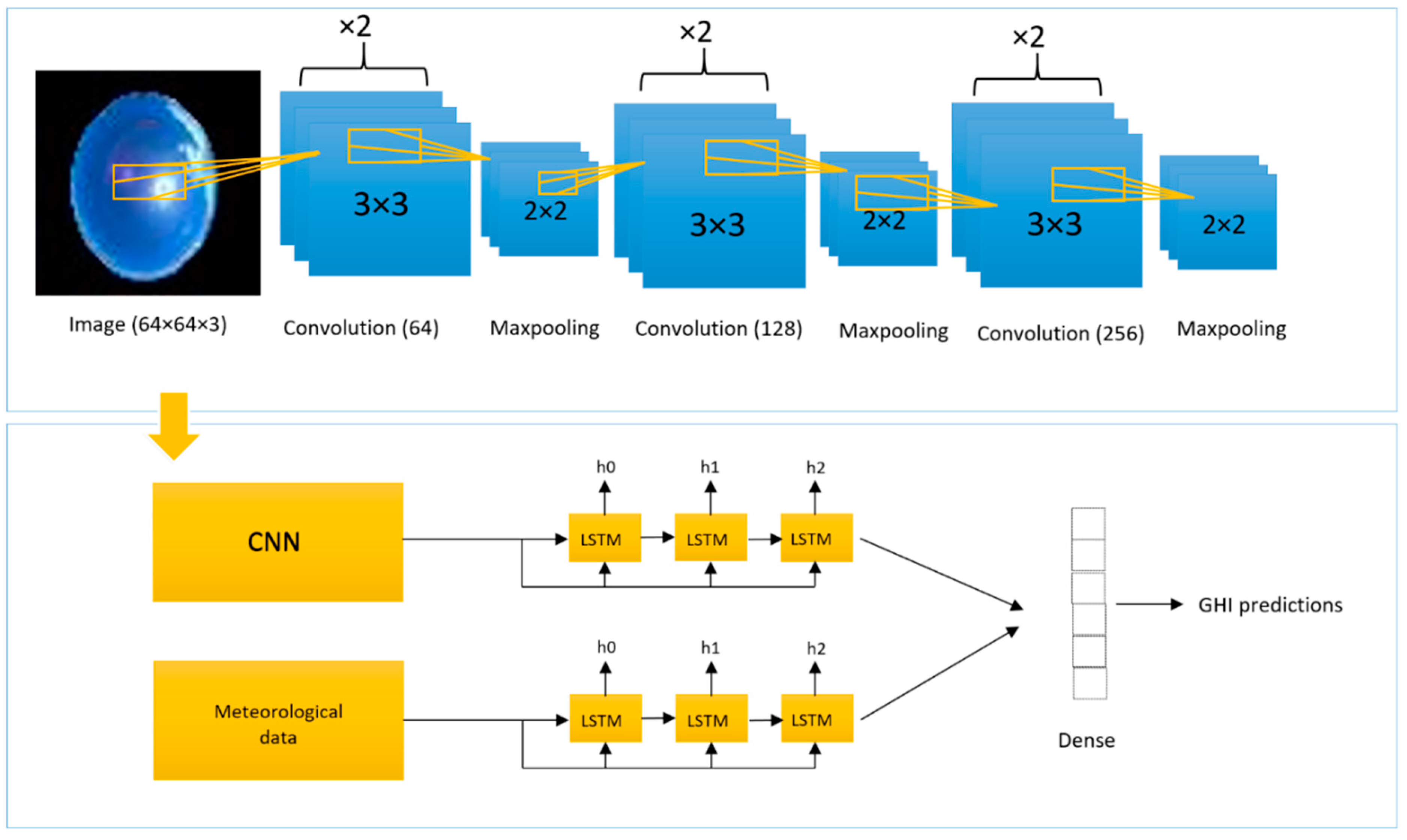
In this article, we implemented a hybrid deep learning model for mean hourly forecasting, using convolutional layers for feature extraction from images and LSTM technology for meteorological data processing and time-series forecasting. The performance of the hybrid model was compared to the performance of three other neural nets, specifically, ANN, CNN, and LSTM. The persistence model was compared to each of the implemented models. The novelty of this study resides in the residual modeling implemented with the CNN-LSTM model, which enables us to generate probabilistic forecasts from the statistical models. Overall, the testing data, for each type of day, and for all the deterministic and probabilistic metrics, the hybrid model was found to be the best performing and most accurate. Indeed, the RMSE, MAE, and R² for the CNN-LSTM were equal to 100.58 W/m², 66.09 W/m², and 0.85, respectively, which is better than the other benchmark models. For probabilistic forecasts, the CNN-LSTM has the best CWC values with 8.54, 17.04, 33.37, and 47.98, respectively, for PI(38%), PI(68%), PI(95%), and PI(99%).

References

1. IEA. Solar PV; IEA: Paris, France, 2022; Available online: https://www.iea.org/reports/solar-pv (accessed on 15 January 2023).
2. Child, M.; Bogdanov, D.; Breyer, C. The role of storage technologies for the transition to a 100% renewable energy system in Europe. In Proceedings of the Energy Procedia, 12th International Renewable Energy Storage Conference, IRES 2018, Düsseldorf, Germany, 13–15 March 2018; Volume 155, pp. 44–60. [Google Scholar] [CrossRef]
3. Yu, Y.; Cao, J.; Zhu, J. An LSTM Short-Term Solar Irradiance Forecasting Under Complicated Weather Conditions. IEEE Access 2019, 7, 145651–145666. [Google Scholar] [CrossRef]
4. Ramsami, P.; Oree, V. A hybrid method for forecasting the energy output of photovoltaic systems. Energy Convers. Manag. 2015, 95, 406–413. [Google Scholar] [CrossRef]
5. Ehara, T. Overcoming PV Grid Issues in the Urban Areas. Switzerland. 2009. Available online: https://www.osti.gov/etdeweb/biblio/22119637 (accessed on 2 January 2022).
6. Husein, M.; Chung, I.-Y. Day-Ahead Solar Irradiance Forecasting for Microgrids Using a Long Short-Term Memory Recurrent Neural Network: A Deep Learning Approach. Energies 2019, 12, 1856. [Google Scholar] [CrossRef] [Green Version]
7. Sun, Y.; Szucs, G.; Brandt, A.R. Solar PV output prediction from video stremas using convolutional neural networks. Energy Environ. Sci. 2018, 7, 1811–1818. [Google Scholar]
8. Jang, H.S.; Bae, K.Y.; Park, H.-S.; Sung, D.K. Solar Power Prediction Based on Satellite Images and Support Vector Machine. IEEE Trans. Sustain. Energy 2016, 7, 1255–1263. [Google Scholar] [CrossRef]
9. Tiwari, S.; Sabzehgar, R.; Rasouli, M. Short Term Solar Irradiance Forecast Using Numerical Weather Prediction (NWP) with Gradient Boost Regression. In Proceedings of the 2018 9th IEEE International Symposium on Power Electronics for Distributed Generation Systems (PEDG), Charlotte, NC, USA, 25–28 June 2018; pp. 1–8. [Google Scholar] [CrossRef]
10. Kambezidis, H.D.; Psiloglou, B.E.; Karagiannis, D.; Dumka, U.C.; Kaskaoutis, D.G. Meteorological Radiation Model (MRM v6.1): Improvements in diffuse radiation estimates and a new approach for implementation of cloud products. Renew. Sustain. Energy Rev. 2017, 74, 616–637. [Google Scholar] [CrossRef]
11. Kambezidis, H.D.; Kampezidou, S.I.; Kampezidou, D. Mathematical Determination of the Upper and Lower Limits of the Diffuse Fraction at any Site. Appl. Sci. 2021, 11, 8654. [Google Scholar] [CrossRef]
12. Akhter, M.N.; Mekhilef, S.; Mukhlis, H.; Shah, N.M. Review on forecasting of photovoltaic power generation based on machine learning and metaheuristic techniques. IET Renew. Power Gener. 2019, 13, 1009–1023. [Google Scholar] [CrossRef] [Green Version]
13. Reikard, G. Predicting solar radiation at high resolutions: A comparison of time series forecasts. Sol. Energy 2009, 83, 342–349. [Google Scholar] [CrossRef]
14. Mora-López, L.; Sidrach-de-Cardona, M. Multiplicative ARMA models to generate hourly series of global irradiation. Sol. Energy 1998, 63, 283–291. [Google Scholar] [CrossRef]
15. Huang, J.; Korolkiewicz, M.; Agrawal, M.; Boland, J. Forecasting solar radiation on an hourly time scale using a Coupled AutoRegressive and Dynamical System (CARDS) model. Sol. Energy 2013, 87, 136–149. [Google Scholar] [CrossRef]
16. Crisosto, C.; Hofmann, M.; Mubarak, R.; Seckmeyer, G. One-Hour Prediction of the Global Solar Irradiance from All-Sky Images Using Artificial Neural Networks. Energies 2018, 11, 2906. [Google Scholar] [CrossRef] [Green Version]
17. Mishra, S.; Palanisamy, P. Multi-time-horizon Solar Forecasting Using Recurrent Neural Network. In Proceedings of the 2018 IEEE Energy Conversion Congress and Exposition (ECCE), Portland, OR, USA, 23–27 September 2018; pp. 18–24. [Google Scholar] [CrossRef] [Green Version]
18. Peng, Z.; Yu, D.; Huang, D.; Heiser, J.; Yoo, S.; Kalb, P. 3D cloud detection and tracking system for solar forecast using multiple sky imagers. Sol. Energy 2015, 118, 496–519. [Google Scholar] [CrossRef]
19. Kuhn, P.; Nouri, B.; Wilbert, S.; Prahl, C.; Kozonek, N.; Schmidt, T.; Yasser, Z.; Ramirez, L.; Zarzalejo, L.; Meyer, A.; et al. Validation of an all-sky imager-based nowcasting system for industrial PV plants. Prog. Photovolt. Res. Appl. 2018, 26, 608–621. [Google Scholar] [CrossRef]
20. Sun, Y.; Venugopal, V.; Brandt, A.R. Convolutional Neural Network for Short-term Solar Panel Output Prediction. In Proceedings of the 2018 IEEE 7th World Conference on Photovoltaic Energy Conversion (WCPEC) (A Joint Conference of 45th IEEE PVSC, 28th PVSEC & 34th EU PVSEC), Waikoloa Village, HI, USA, 10–15 June 2018; pp. 2357–2361. [Google Scholar] [CrossRef]
21. El Alani, O.; Abraim, M.; Ghennioui, H.; Ghennioui, A.; Ikenbi, I.; Dahr, F.-E. Short term solar irradiance forecasting using sky images based on a hybrid CNN–MLP model. Energy Rep. 2021, 7, 888–900. [Google Scholar] [CrossRef]
22. Kolen, J.; Kremer, S.C. Gradient Flow in Recurrent Nets: The Difficulty of Learning LongTerm Dependencies; Wiley-IEEE Press: Hoboken, NJ, USA, 2001. [Google Scholar] [CrossRef] [Green Version]
23. Hochreiter, S.; Schmidhuber, J. Long Short-Term Memory. Neural Comput. 1997, 9, 1735–1780. [Google Scholar] [CrossRef]
24. Dobbs, A.; Elgindy, T.; Hodge, B.-M.; Florita, A.; Novacheck, J. Short-Term Solar Forecasting Performance of Popular Machine Learning Algorithms; National Renewable Energy Laboratory: Jefferson County, CO, USA, 2017. [Google Scholar]
25. Ghimire, S.; Deo, R.C.; Raj, N.; Mi, J. Deep solar radiation forecasting with convolutional neural network and long short-term memory network algorithms. Appl. Energy 2019, 253, 113541. [Google Scholar] [CrossRef]
26. Kumari, P.; Toshniwal, D. Extreme gradient boosting and deep neural network based ensemble learning approach to forecast hourly solar irradiance. J. Clean. Product. 2021, 279, 123285. [Google Scholar] [CrossRef]
27. Li, X.; Ma, L.; Chen, P.; Xu, H.; Xing, Q.; Yan, J.; Lu, S.; Fan, H.; Yang, L.; Cheng, Y. Probabilistic solar irradiance forecasting based on XGBoost. Energy Rep. 2022, 8, 1087–1095. [Google Scholar] [CrossRef]
28. He, H.; Lu, N.; Jie, Y.; Chen, B.; Jiao, R. Probabilistic solar irradiance forecasting via a deep learning-based hybrid approach. IEEJ Trans. Electr. Electron. Eng. 2020, 15, 1604–1612. [Google Scholar] [CrossRef]
29. Carrière, T.; Amaro e Silva, R.; Zhuang, F.; Saint-Drenan, Y.-M.; Blanc, P. A New Approach for Satellite-Based Probabilistic Solar Forecasting with Cloud Motion Vectors. Energies 2021, 14, 4951. [Google Scholar] [CrossRef]
30. Nielsen, A.H.; Iosifidis, A.; Karstoft, H. IrradianceNet: Spatiotemporal deep learning model for satellite-derived solar irradiance short-term forecasting. Sol. Energy 2021, 228, 659–669. [Google Scholar] [CrossRef]
31. Ineichen, P.; Perez, R. A new airmass independent formulation for the Linke turbidity coefficient. Sol. Energy 2002, 73, 151–157. [Google Scholar] [CrossRef] [Green Version]
32. Vii, T. Etude de l’Eclairement et du Potentiel Photovoltaïque à l’Université de la Polynésie Française: Etude Météorologique et Modélisation de Système Photovoltaïque. University of French Polynesia: Puna’auia, French Polynesia, 2020. [Google Scholar]
33. Siddiqui, T.A.; Bharadwaj, S.; Kalyanaraman, S. A Deep Learning Approach to Solar-Irradiance Forecasting in Sky-Videos. In Proceedings of the 2019 IEEE Winter Conference on Applications of Computer Vision (WACV), Waikoloa Village, HI, USA, 7–11 January 2019; pp. 2166–2174. [Google Scholar] [CrossRef] [Green Version]
34. Jayalakshmi, N.Y.; Shankar, R.; Subramaniam, U.; Baranilingesan, I.; Karthick, A.; Stalin, B.; Rahim, R.; Ghosh, A. Novel Multi-Time Scale Deep Learning Algorithm for Solar Irradiance Forecasting. Energies 2021, 14, 2404. [Google Scholar] [CrossRef]
35. Dumas, J.; Cointe, C.; Fettweis, X.; Cornélusse, B. Deep learning-based multi-output quantile forecasting of PV generation. In Proceedings of the 2021 IEEE Madrid PowerTech, Madrid, Spain, 28 June–2 July 2021; pp. 1–6. [Google Scholar] [CrossRef]
Figure 1. Total sky imager with a digital camera Axis 212 PTZ (left). Sky image taken at the University on 3 November 2019 (right).
Atmosphere 14 01192 g001
Figure 2. Pearson correlation test for the measured meteorological data.
Atmosphere 14 01192 g002
Figure 3. GHI autocorrelation using the Pearson correlation, for a time-shift ranging from 0 to 300 min. Red cross representing the Pearson coefficient.
Atmosphere 14 01192 g003
Figure 4. Implemented CNN, with inputs being image sequences and meteorological data. The output is the predicted GHI for the next hour.
Atmosphere 14 01192 g004
Figure 5. Implemented CNN-LSTM. The sky images are first processed by a CNN, then by an LSTM. The meteorological data are only processed by the LSTM. The two LSTMs are concatenated into a dense layer for GHI predictions.
Atmosphere 14 01192 g005
Figure 6. Distribution of residuals at 10 am (left) and 13 pm (right).
Atmosphere 14 01192 g006
Figure 7. GHI measurements versus predictions for data test n°1.
Atmosphere 14 01192 g007
Figure 8. Probabilistic predictions for the hybrid model for PI(38%), PI(68%), PI(95%), and PI(99%).
Atmosphere 14 01192 g008