Abstract
In cases of accidental or deliberate incidents involving a harmful agent in urban areas, a detailed modelling approach is required to include the building shapes and spatial locations. Simultaneously, when applied to crisis management, a simulation tool must meet strict time constraints. This work presents a Lagrangian particle model (LPM) for computing atmospheric dispersion. The model is implemented in the nuclear decision support system ESTE CBRN, a software tool developed to calculate the atmospheric dispersion of airborne hazardous materials and radiological impacts in the built-up area. The implemented LPM is based on Thomson’s solution for the nonstationary, three-dimensional Langevin equation model for turbulent diffusion. The simulation results are successfully analyzed by testing compatibility with Briggs sigma functions in the case of continuous release. The implemented LPM is compared with the Joint Urban 2003 Street Canyon Experiment for instantaneous puff releases. We compare the maximum concentrations and peak times measured during two intensive operational periods. The modeled peak times are mostly 10–20% smaller than the measured. Except for a few detector locations, the maximum concentrations are reproduced consistently. In the end, we demonstrate via calculation on single computers utilizing general-purpose computing on graphics processing units (GPGPU) that the implementation is well suited for an actual emergency response since the computational times (including dispersion and dose calculation) for an acceptable level of result accuracy are similar to the modeled event duration itself.
1. Introduction
A crisis management mission is a quick, confident and complex response to harmful events. One such mission is the application of adequate mitigating measures. This goal is achievable if the decision making is based on a detailed understanding of the current situation. Therefore, modelling tools are very helpful in these situations.
The ESTE CBRN software tool is a nuclear decision support system designed to model the radiological impacts of a radiological or nuclear event in urban areas. The software aims to identify and calculate the corresponding wind field; specifically, this software is used to perform atmospheric dispersion and radiological impact calculations. In the original approach, the atmospheric modelling in ESTE CBRN was based on Gaussian modelling in combination with a puff trajectory model. This approach is also applied in several other fast-response systems, e.g., in SCIPUFF (the Second Order Closure Integrated Puff model) [1]. The Gaussian approach has short simulation times and low requirements for implementation in urban area because it models the urban environment only partially and does not include 3-dimensional models of buildings. In ESTE CBRN, the Gaussian formulation of urban atmospheric dispersion is expressed by urban sigma functions [2,3].
Dispersion modelling characterized as 3-dimensional is achievable using the Eulerian or Lagrangian approach. Using one of these approaches, with the building locations and their shapes, the calculation can be performed in detail when required. An existing limitation is the amount of computational resources available and the requirement on the calculation duration.
In addition to the Gaussian model of the ESTE system, a 3D approach for the dispersion modelling in ESTE was implemented using a Eulerian model [4]. This 3D model of the ESTE system was validated in the UDINEE project (Urban Dispersion International Evaluation Exercise, [5,6]) against the Joint Urban Experiment JU2003 performed in Oklahoma City (USA). In that project, we compared the urban wind field computational model and the Eulerian approach implemented in ESTE with measured meteorological data and concentrations of SF6 [4]. The compliance of the modeled and measured data was moderate. Many variables compared, such as puff arrival time, are generally well reproduced and fulfil the urban modelling criteria. However, the calculation duration using the Eulerian approach did not comply with emergency requirements. This disadvantage motivated us to replace the Eulerian model with the Lagrangian dispersion model in the ESTE CBRN to satisfy the requirements to perform a 3D calculation approach for emergency purposes.
The Lagrangian particle model implemented is based on Thomson’s simplest solution for the nonstationary, three-dimensional Langevin equation model [7]. This approach (and similar models) is applied in other software systems, such as QUIC-PLUME [8], UrbanLS [9,10] and P-SPRAY [11].
In the present work, we focus on validating the LPM as a proper atmospheric model tool in an urban environment. The validation is performed mainly on the JU2003 experimental data, where we show that the LPM implemented in ESTE CBRN is appropriate for urban dispersion modelling.
The ESTE CBRN system is not only an atmospheric transport modelling system; it is also a system for radiological consequence calculations, with the impact calculation assuming all exposure pathways. The calculation of external effective doses due to ground shine and cloud shine are performed on the same 3D computational domain of the modeled urban area on which the corresponding atmospheric transport calculation is performed. This method of implementation enables us to take into account 3D modelling of buildings in three phases (calculation of wind field, calculation of dispersion and calculation of external exposure). Three-dimensional modelling of buildings is the key for including their shielding effects in the calculation of external exposure.
The ESTE CBRN system models several types of CBRN events, but it focuses on the modelling of the radiological dispersal device (RDD). Events with the RDD represent a special type of radiological event. The database of RDD events implemented in ESTE CBRN consists of (i) a model for a classical radiological dispersal device (CRDD), (ii) a model for an improvised burned-up nuclear fuel dispersion device (INFDD), (iii) a model for a mortar dispersing pulverized chemical compounds of radioactive nuclides, and (iv) a model for an improvised nuclear device (IND).
In this study, we focus on the creation of complex system for emergency response. Such systems must fulfill strict computational time constraints (results could be available in, for example, 15–20 min), and acceptable accuracy of results. One option to achieve these goals is the application of large computer clusters, which provide the capability for fast computing and the capability to cover large geographical areas [12]. Another option is to utilize the technology of GPGPU, which offers a massive parallel computing approach. We show that a Lagrangian particle dispersion model coupled with a radiological impact calculation, both implemented using GPGPU technology, is a time-efficient method to perform accurate and short-duration calculations.
In the present study, we do not analyze the calculation of the urban wind field. Some original approaches are designed to run fast [13], a compromise between computational accuracy and a real-time approach. Another approach represents the direct application of CFD (Computational Fluid Dynamics) techniques. In the case of ESTE CBRN, the urban wind field is calculated through a CFD model using Reynolds-averaged Navier–Stokes (RANS). The CFD approaches are more accurate but also more time-consuming. Here, one option is an application of supercomputing resources. Another option is to have a well-designed set of pre-calculated wind fields for a particular urban area prepared in advance. The application of pre-calculated wind fields was realized for the Operational Canadian Urban Dispersion Modelling (CUDM) System, in the case of the principal Canadian towns [14]. A pre-calculated database of wind fields is also applied in the ESTE CBRN.
The structure of the present work is as follows: In Section 2 (Modelling Approach), we describe the applied Lagrangian particle models together with a short description of the wind field calculation applied. Furthermore, we describe the radiological model for the calculation of the basic radiological parameters caused by the relevant exposure pathways. In Section 3, we present the validation tests of the LPM implemented in ESTE CBRN. The first test is a simple comparison against empirical formulas of Briggs sigma functions; the second test is a comparison against the JU2003. In this section, we also analyze the application of the whole calculation model, including the Lagrangian particle model and radiological impact model, as a system running on GPU as a real-time running system for emergency response. Finally, in Section 4 we provide a summary.
2. Modelling Approach
2.1. Modelling of Dispersion in Urban Atmosphere
Lagrangian particle models describe transport and dispersion by modelling particle motion inside a wind field composed of two components, a mean wind and a turbulent wind. The new positions of the particles (in general noted as ) are given by the following equations:
where Δt is the time step; u, v and w (in general noted as ) are components of Lagrangian velocity; U, V and W (in general noted as ) are components of the mean (Eulerian) wind field; and uf, vf and wf (in general noted as ) are the fluctuating components of Lagrangian velocity. The fluctuating velocity component follows Thomson’s equations [15]:
where dWj(t) is an incremental of the Wiener process; ai is the i-component of the deterministic term; and bij are the stochastic coefficients. In the equations we assume summation over j, from 1 to 3.
The implemented LPM is based on Thomson’s simplest solution, which represents a simplification of Thomson’s solution for the nonstationary, three-dimensional Langevin equation model for turbulent diffusion. In the case of rotating the coordinate system into the direction of the mean wind field, the fluctuating velocity components have the forms (here, assume rotation into the x direction; thus, Vr = Wr = 0, where the subscript r means variable in the rotated system) [7]:
where C0 is the universal constant for the Lagrangian structure function. While sources refer to various ranges for this constant, we applied the value 5.6 [7]. ε is the mean rate of turbulence kinetic energy dissipation. dWj are uncorrelated, normally distributed variables with mean values of zero and standard deviations equal to 1. The components of the inverse tensor λij are given by the following formulas:
where τij are the components of the Reynolds stress tensor, which are defined using the variances of the velocity τ11 = σu2, τ22 = σv2, τ33 = σw2 and the Reynolds shear stress τ13 = τuw.
In our approach, the mean field,, the Reynolds stress tensor, τij, and kinetic energy dissipation, ε, are calculated numerically as a solution of the Reynolds-averaged Navier–Stokes (RANS) equations of buoyant and incompressible fluid with the Boussinesq hypothesis. For not assuming the temperature variances, the complete fluid equations were reduced to the following form:
where ν is the kinematic viscosity; νt is the turbulent kinematic viscosity; ρ is the density; δij is the Kronecker delta symbol; and k is the turbulent kinetic energy. Our approach focuses on the steady-state solution. Thus the time derivate term in Equation (11) is omitted. Equations (11)–(13) are solved using the approach of the SIMPLE algorithm (Semi-Implicit Method for Pressure-Linked Equations, [16]). The turbulence closure considered is the standard k–ε turbulence model. The calculation is performed using the OpenFOAM framework (available at URL https://www.openfoam.com/ (accessed on 23 June 2023)). The description of the boundary conditions depends on the known wind speed, friction velocity and Obukhov length, which are determined from the measured meteorological conditions [4].
The locally determined Reynolds tensor from (11)–(13) is regularized by transforming the Reynolds tensor into the coordinate system in which the main direction is defined by the mean wind field, and then by fitting it to the following form:
where we assume k1 = 4, k3 = 1.32 = 1.7. This setting is well defined for a neutral condition [3] and applicable for stable and unstable conditions as an acceptable approximation. A similar parametrization is applied in [8].
In a real situation, we are faced with various types of events leading to various properties of airborne particles. A basic characteristic of a dispersed particle is that its size has a significant impact on the particle’s motion in the turbulent wind field. Three categories of particles are assumed [3]:
- (i)
- Particles with radii smaller than 5 μm and gases: Gravitational settling can be neglected due to their small particle size; thus, the flow in the mean wind field and the dispersion are dominant and considered in the calculation, while gravitational settling is not.
- (ii)
- Particles with radii between 5 μm and 80 μm: Gravitational settling is non-negligible; thus, it is considered in the flow in the mean wind field and in the dispersion. Gravitational settling is represented by the terminal velocity vt, given as (Stoke’s law):
- (iii)
- Particles with radii greater than 80 μm: The main effect determining the vertical motion is gravitational settling. The gravitational fall begins at zero velocity and is described by the equation (Stoke’s law for a small sphere):
Deposition on surfaces is also treated with respect to the particle size:
- (i)
- Particles with radii smaller than 80 μm: Each particle has its settling velocity. For particles larger than 5 μm, the settling velocity is approximated using their terminal velocity. For particles smaller than 5 μm, the settling velocity is approximated with a curve expressing the dependence between the particle radius and settling velocity (according to [3]). When the bottom face of the particle’s cell is a ground surface, the particle leaves one part of its activity on the surface. This part of the activity is expressed using the settling velocity as:
- (ii)
- Particles with radii greater than 80 μm: When crossing a horizontal surface, the particle is deposited totally because its contact with the surface is due to gravitational fall. When crossing a vertical surface, it is reflected by a specified probability. Otherwise is deposited totally. The probability of reflection is set to 85% (based on [17]).
2.2. Applied Computational Domain
In our study, with a focus on validation and analysis of applicability for emergency responses, we performed calculations for several sites. For each site, we applied the corresponding computational domain. All the calculation domains were prepared to perform a realistic calculation of atmospheric transport for the given modeled locations.
The simplest location was the area of the multi-unit nuclear power plant (NPP) in Mochovce, Slovakia. The location consists of several large buildings, including eight cooling towers, four reactor buildings, and many smaller buildings. The calculation domain, already applied in our study [18], has 377,474 cells and covers an area of 2.8 km × 1.4 km × 1 km. The horizontal dimensions of the cell are 20 m × 20 m. The parameters of the computational models are listed in Table 1.

Table 1.
Basic parameters of the applied computational domains.
The largest model is represented by the calculation model of downtown Oklahoma City (OK, USA). It has 4,029,620 cells and covers an area of 1.4 km × 1.65 km × 194 m. The horizontal dimensions of the cell are 5 m × 5 m. The height of the cells varied between 1 m (for the layer near the terrain) and 16 m for the uppermost layer. This computational model, applied already in our previous study [4] within the UDINEE project, reflects the urban situation in 2003, since its main purpose is to provide a comparison with JU2003.
The third location studied is the historical center of Kosice, Slovakia. It is an urban area with a large number of middle-sized buildings and many streets. The computational domain was created using the OSM Buildings data. The domain contains 1,684,925 cells (with a cell size of 7 m) and covers an area of 1.3 km × 1.7 km × 189 m. Its parameters are summarized in Table 1. The actual location of the modeled area is shown in Figure 1, and the prepared computational domain is shown in Figure 2. In the study, the modeled historical center of Kosice was used to test the applied dosimetric algorithms.
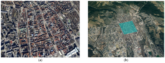
Figure 1.
Views of the city center of Kosice. (a) A closer view directly on the modeled area; (b) A distant view with a visualized domain area (in blue).
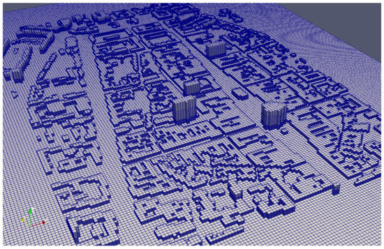
Figure 2.
The city center of Kosice as visualized in the orthogonal computational mesh, using [19].
A special calculation domain was prepared for the comparison to Briggs sigma functions. Its resolution is 20 m in the horizontal direction and 5 m in vertical resolution. The domain size was 5000 m × 1000 m × 500 m (=length × width × height). The domain does not include any buildings.
2.3. Modelling of Urban Conditions Using Empirical Briggs Formulas
Modelling of atmospheric transport in an urban environment can also be performed in a simplified approach when the real positions of the buildings are considered. In such a case, the wind field is defined uniformly in the horizontal direction and with adequate analytic formulas for vertical profiles (or with a measured vertical profile).
In this simplified approach, we analyze our implemented LPM. We perform calculations for neutral and stable conditions. The wind fields and turbulent fields in the computational domain at neutral and stable conditions are defined by equations [3]:
where the constant κ = 0.4 is von Karman’s constant; is the friction velocity; z is the height above the terrain; z0 is the surface roughness; and u is the wind at the height of z. The component of the Reynolds stress tensor, R, under neutral conditions is expressed as parametrized in [3]. Rm is equal to 1 in neutral conditions (neglecting the Coriolis corrections for assuming small heights), and it is equal to (1 − z/zi) in stable conditions. The parameter zi represents the inversion height. hm is equal to 1 in neutral conditions, and it is equal to (1 + 5z/L) in stable conditions. em is equal to 1 in neutral conditions, and it is equal to (1 + 4z/L) in stable conditions. L is the Monin-Obukhov length.
The surface roughness represents a parameter with which we can model the presence of buildings very generally, although it is not really in the model. We vary the surface roughness between 0.07 (corresponding to a locality with an almost flat terrain) and 1.0 (corresponding to an area with buildings).
In such a setting, we model a continuous release in a specific height above the ground. The atmospheric transport modeled through LPM under the described simplified urban and rural conditions has to be consistent with the Briggs plume sigma functions for urban and rural conditions [2]. These functions represent widely accepted plume behavior. They express the functional dependencies of standard deviations of concentration on the distance from the release point in vertical and lateral directions, as summarized in Table 2.
Table 2.
The dependence on the downwind distance of the Briggs sigma functions for various stability categories and environmental conditions (rural, urban).
2.4. JU2003 Experiment
The primary comparison of the implemented LPM was performed using the experimental data from Joint Urban 2003, conducted July 2003 in Oklahoma City, USA e.g., [20,21]. The experiment consisted of ten Intensive Observation Periods (IOPs) during which SF6 was released as a tracer gas and its concentration was measured at various locations in downtown Oklahoma City.
Our validation study analyzed the instantaneous puff releases of IOP 3 and IOP 5. The basic input data is taken from [20], including the release setup, meteorological data and tracer measurements. The puff releases of IOP 3 were performed through balloon bursting, with the corresponding SF6 mass of 1000 g at the height of 2 m above the ground. The focus of our study was the first three puff releases, which started at 9:00, 9:20 and 9:40, respectively (all times are in CDT, central time zone). The puff releases of IOP 5 were conducted the same way, but the applied release masses were 500 g. The corresponding start times were 15:00, 15:20 and 15:40, respectively. Both IOPs were situated at the same location, near the Botanical Gardens (see Figure 3).
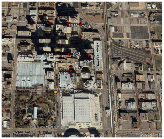
Figure 3.
Downtown Oklahoma City. Displayed are the locations of the TGA tracers for IOP 3 and the release points (yellow circles).
The tracer measurement data included locations of samplers and their maximum reported concentrations (in pptv, parts per trillion volume). The instantaneous concentrations were measured using Trace Gas Analyzers (TGAs) with a frequency of 2 Hz. The upper measurement range varied between 11,000 pptv and 23,000 pptv. The lower limit was about 150 pptv (MLOD).
The meteorological data used in our study were also taken from [20], where the 15-min averages of sodar winds at 100-m AGL are provided. The meteorological measurements were used to define the boundary conditions based on [3,22]. The wind and turbulence fields for the computational domain of Oklahoma City were calculated by applying computational fluid dynamics techniques. Specifically, the wind fields resulted as solutions of the Reynolds-averaged Navier–Stokes equations for buoyant, incompressible fluid using the Boussinesq approximation [4]. The turbulence is governed by the standard k–ε model.
This approach to the urban wind field calculation was applied in our earlier analysis of JU2003 [4]. There, we showed that our method of wind field calculation was applicable. The ratio of the modeled to the measured value of the wind speed measurements inside the downtown area was close to unity, and the count of this ratio, being between 0.5 and 2.0 (expressed as the variable factor of 2, FAC2), was equal to 80%. The turbulent kinetic energy was generally underestimated by 30–40%.
2.5. Modelling of Radiological Effects
A set of radiological parameters is modeled and calculated. The most important for radiological impacts are effective doses from external exposure and committed effective doses from inhalation. The radiation exposure occurs: (i) during the initial phase and passage of the cloud and (ii) after the passage of the cloud. The first group of radiological parameters include external irradiation from the cloud, external irradiation from the deposited material and internal irradiation via inhalation of airborne radioactive particles and gases. After the passage of the cloud, external exposure from deposited radionuclides on the ground and walls and internal exposure from inhalation of resuspended radioactive material are considered.
The dose rate DRinhal of the committed effective dose by inhalation is calculated for a considered radionuclide n as:
where Ct(n,x) is the short-time average concentration at the point of interest x in time t. BR is the breathing rate, depending on age. CFinhal is the conversion factor for the committed effective dose due to inhalation, depending on age and nuclide. The integral dose is calculated by using the corresponding time-integrated concentration. In a numerical approach, the concentration in a given location is equal to the concentration value in the corresponding computational cell.
DRinhal (n, age, x, t) = Ct(n,x) CFinhal (age,n) BR(age).
The dose rate DRdepo of the external dose by fallout is calculated for a considered radionuclide n as:
where Dt(n,x) is the deposition value (in Bq/m2) at time t and location x. The calculation represents the summation over all the terrain and building surfaces of the calculation domain. The CFdepo(n,x,y) is the external dose conversion factor for deposition (external dose at point x from the surface at point y). The SF(x,y) is the shielding factor, representing the shielding effect of the buildings. In our approach, it is equal either to 1, if there is no obstacle (e.g., a building), or to 0, if there is at least one obstacle along a straight line between point x and the surface of point y. The corresponding integral dose is calculated by the summation Σt Δt DRdepo(n,x,t), where we sum the corresponding time interval.
DRdepo (n,x,t) = Σdomain,y Dt (n,y) CFdepo(n,x,y) SF(x,y).
To calculate deposition doses on the calculation domain, the surface deposition Dt(n,x) in the given location equals the surface activity value on the corresponding computational surface tile (=ground or building). The shielding factor SF(x,y) is calculated by applying the Muller-Trumbore intersection algorithm [23]. This algorithm is applied in order to reduce computational time. The calculation considers each pair of tile centers where one center is the source and the other is the receiver, with each building surface tile used as a tested shielding object. The CFdepo(n,x,y) is represented by a library of pre-calculated factors. This factor is equal to the impact (=effective dose) caused by a tile of unit surface activity located between 1 m and 2000 m from the point of interest. The library was prepared using numerical simulations in MCNP 5 [24].
The dose rate DRcloud of the external dose by cloud shine is calculated for the considered radionuclide n as:
DRcloud (n,x,t) = Σdomain,y Ct(n,y) CFcloud(n,x,y) SF(x,y).
The CFcloud(n,x,y) is the cloud analogy to CFdepo(n,x,y). It is the conversion factor for external exposure at point x caused by airborne activity at point y. Similar to CFdepo(n,x,y), CFcloud(n,x,y) is represented by a library of pre-calculated factors. The calculation is performed the same way for ground shine. The volume concentration Ct(n,y) in the given location is equal to the cell concentration value. The calculation considers each cell center the source, each bottom surface tile the impacted point and each building surface tile a tested shielding object.
3. Results
3.1. Model Comparison to Briggs Formulas
The first test of our implementation was performed in a quasi-urban approach. The surface was represented by a plain without a building. We applied the calculation domain with a flat terrain, described in Section 2.2. The turbulence and wind fields were determined using analytic formulas for vertical profiles, defined by the Equations (18)–(20). The modeled dispersion results were compared to the Briggs plume sigma functions for urban and rural conditions [2]. To validate the implemented LPM, we focused on neutral conditions and stable conditions. In the case of neutral conditions, we generated several states of meteorological conditions. We modeled a continuous release at the height of 50 m above ground. We generated a couple of meteorological conditions to show that the LPM aligns with the Briggs sigma functions. In the case of neutral conditions, we analyzed two cases for the wind speed: one moderate value of wind speed (2.4 m/s) and one higher value (4.8 m/s). Three distinct values of surface roughness were assumed, 0.07, 0.3 and 1.0, covering areas from flat terrain through small buildings and large buildings.
For the modeled plume, we evaluated the first and second moment (i.e., the mean and variance) of the spatial distribution of the concentration in air as a function of the distance from the release point separately in the horizontal lateral direction and in the vertical direction. The resulting variance σ was compared to the Briggs formulas. They are expressed in a general form of Ax(1 + Bx)c, where c is either −0.5 or −1, depending on the weather conditions (see Table 2). The analysis is focused on parameter A, which primarily determines the behavior at small and medium distances.
For surface roughness 1.0 at neutral conditions, we obtained A of about 0.15 in the lateral direction, which is close to the value of 0.16 for the urban σy. In the vertical direction, the interpolated value of A is about 0.11, which is again close to the urban Briggs σz value of 0.14. For the surface roughness of 0.07 at a neutral condition, we obtained A of about 0.063 in the lateral direction and 0.042 in the vertical direction. These values are consistent with the coefficients for rural conditions, which are 0.08 and 0.06 (in lateral and vertical directions, respectively). In all cases, the results show low dependence on wind speed. The order of magnitude of interpolated values of parameter B is comparable with the Briggs formula. Interpolated B is satisfactorily small. A more accurate determination of B is beyond the range of our analysis. An overview of the meteorological conditions considered and the resulting interpolated coefficients are listed in Table 3.
Table 3.
Input parameters for model comparison with Briggs sigma functions and the resulting interpolated values of coefficients of Briggs sigma functions.
The dependencies on the distances from the release point modeled by LPM and predicted by the Briggs formulas are presented in Figure 4. The results of LPM implemented in ESTE for high surface roughness reproduce the analytical dependencies for urban conditions sufficiently. Similarly, the modeled results for low surface roughness reproduce the analytical behavior in rural conditions. The case with an intermediate surface roughness value represents the middle ground between the urban and rural conditions. As for neutral conditions, we obtained a similar consistency between the Briggs sigma functions and the modeled variance of stable conditions (see Table 3).
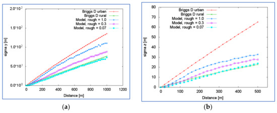
Figure 4.
Comparison of Briggs sigma functions for stability category of D, with modeled dispersion by LPM at various levels of surface roughness. (a) Comparison of dispersion in lateral (y) direction; and (b) Comparison of dispersion in vertical (z) direction.
In Figure 4, we identify one interfering effect influencing dispersion in the vertical direction. The release is situated at a height of 50 m. The performed analyses can be relevant only to the distances where the plume reaches the ground or the upper boundary. The plume reflects effectively by reaching such a surface. The calculated variance beyond this distance does not represent the situation expressed by the analytical formulas. In the case of urban conditions, Briggs z-sigma is 25 m at the approximate distance of 150 m; at this distance, the plume reaches the boundaries (2 × σz = 50 m). Therefore, the curve of the modeled variance is more deviated from the analytical lines in the case of dispersion in the vertical direction, and the modeled curve bends beyond the distance of about 200 m considerably. This is not the case with the horizontal dispersion because the test computational domain is sufficiently wide to avoid reflecting in the y-direction. This allows us to test the behavior of the plume up to a downwind distance of about 600–700 m.
3.2. Model Comparison to JU2003 Experiment
Our comparison to the JU2003 experiment consists of two steps. First, we determined the urban wind and turbulence fields for the given IOP. Second, we performed the atmospheric transport calculations and finished with comparisons of modeled detector responses with the measured responses. We focused on the calculation of the maximum values of the detectors and the times when the maximum concentrations were reached (i.e., the peak times).
We calculated the steady-state flow during the specific hours when the puff releases occurred; specifically, we calculated the mean hour flow field from 9:00 to 10:00 h for IOP 3 and the mean hour flow field from 15:00 to 16:00 h for IOP 5. The application of the hourly mean field has the effect that our modeled tracer measurements reflect: the mean maximum values over all three puff releases occurred in a specific hour. Similarly, the modeled peak times are compared to the mean peak times. We omit the approach to model each separate puff release because modelling each puff requires working with more detailed meteorological data that is unavailable in our analyses. The puff movements lasted about 5 min in the neighboring vicinity where the detectors were distributed. The applied meteorological data [22] were 15-min averages. Instead of assuming negligible fluctuations (such an assumption is potentially false) of the wind field within 15 min when performing a direct comparison with separate puff releases, we assumed that three puff releases could represent an ensemble to evaluate the mean behavior corresponding to the hourly mean meteorological conditions. To support this approach, we emphasize that the releases occurred close to the edges of buildings, dividing the puff transport into different streets. Therefore, unmeasured small time-scale fluctuations could negatively affect comparison on the level of separate puff releases.
We applied 30,000,000 particles in the validation. Such a high number was required to gain the statistical resolution comparable with the lower measurement. The measurement range was from 150 pptv to about 12,000 pptv. The achieved resolution of the concentration calculation was on the level of 100–200 pptv.
The modeled values of maximum tracer responses are summarized in Table 4. To help our analysis, we follow detectors’ positions compared to the modeled puff transport. Figure 5 visualizes the time integral of concentration in air 2 m above the ground. Here, the puff trajectory at this vertical level is called the approximate continuous region of the highest time integrated concentration, starting at the release point, continuing along several streets, and ending when leaving the domain. Naturally, the puff movement follows the street canyons first and the mean wind field later when moving in the region without a dominant built-up area. In all cases, we evaluated the uncertainty of the modeled values in addition to the estimation of the statistical error. The uncertainty is based on the variation of the calculated maximum concentration in the cell defined by the location of a detector and its neighboring cells. This estimated variance (=uncertainty) is given in Table 4.
Table 4.
Maximum measured TGA-sampled concentrations (pptv), taken from [21], compared to modeled values.
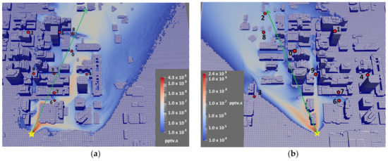
Figure 5.
The modeled time integral of concentration [pptv.s] for IOP 3 (a) and for IOP 5 (b). The release points (yellow star), the locations of the TGA tracers (red circles) and hourly mean wind direction (green arrow) for both IOPs are displayed too.
In the case of IOP 3, the closest tracers to the puff trajectory are measurements 0, 4, 6 and 7. The mean measured maximum values for 4, 6 and 7 are bounded only from the bottom (outside the range of the TGA sampler), and the corresponding values modeled by the LPM are also above the reported range of the TGA sampler. Measurement 0 is sufficiently far from the release point, and here the mean maximum value is measured and modeled consistently. Measurements 1 and 8 are slightly farther from the puff transport, and we obtained underestimated values for them. Measurements 3 and 9 are far from the modeled puff trajectory. The actual measurements provided oscillated maxima, which suggest that they were on the edge of the real puff transport. They were once affected and once not. The modeled values are comparable with those for some puffs, but the mean values were again underestimated. Measurements 2 lies farther away, and the measured and modeled values are at the level of 0 pptv.
In the case of IOP 5, the closest tracer to the release point is measurement 9, and both modeled and measured maxima are correspondingly above the detection capabilities. Measurements 2 and 8 are the farthest; they are located at the end of the highly built-up area and in the direction of the mean wind from the release point. The modeled maximum concentrations are consistent with the mean measured value. In the cases of measurements 6 and 7, the modeled maxima are close to the medium maximum value (the middle value when ordered from the smallest to the largest), but far when compared to the mean value. Measurements 1 and 4 lie visibly far from the expected puff transport. Both are modeled as having a negligible maximum concentration, which is the case for measurement 1 but not for measurement 4. Measurement 2 is located farther away, and the measured and modeled values are at the level of 0 pptv. Finally, measurement 0 has three almost stable maxima, and the modeled value is underestimated by more than a factor of 2.
To summarize, for the close measurements, which lie along the puff movements, the measured maxima are clearly above the detection range, and the modeled results were also above said range. For the distant measurements in the direction of the mean wind, the modeled maxima are mostly within a factor of 2. The measurements lying aside are reproduced partially (i.e., in some cases, the measurements fluctuate, and these fluctuations have no footprint in the modeled results). They could not be present because the wind field calculation as a one-hour mean already removes them. An additional finding is that the model has a small agreement in the case of cross streets, such as measurement 0 for IOP 5 (underestimated 7-fold) or measurement 3 for IOP 3 (underestimated 2.5-fold).
The second quantity we compared was the times when the maximum values of the tracer concentration were reached, the so-called peak time. Here, we made some objective data selections because not all measurements were fully applicable for the peak time analyses because either the modeled or/and the measured peaks were present (such as measurement 2 for IOP 3).
For IOP 3, we analyzed measurements 0, 1, 3, 4 and 6. In measurement 1, the modeled cloud missed the measurement location, as mentioned above; thus, a comparison was not done. For measurements 0 and 3, the ratio between the modeled and measured times is 0.8. For measurements 4 and 6, the time of the maximum value is estimated due to the maximum value overreaching the limit of the detector. These estimated ratios between the modeled and measured peak times range from 0.4 to 0.7.
The same comparison was performed for IOP 5. For measurements 0, 2 and 8, the ratios between the modeled and measured times are 0.8, 1.1 and 1.0, respectively. All these measurements lie close to the line of the wind direction. For measurements 6, 7 and 9, the ratios of the modeled and measured peak times are 0.4, 0.7 and 0.6, respectively. As specified above, these three measurements lie more or less aside, and the modeled peak times are underestimated. These ratios were approximated because the time series had missing values when the concentration was above the upper limit. Measurement 4 was not analyzed because the modeled response was zero. In measurement 1, there were neither measured nor modeled actual peak times.
In general, we see that the peak times were reproduced acceptably. When the peak time is measured and determined, we obtain the ratio model vs. observation approximately equal to 0.9; in other words, we underestimated the peak time by 10%. When the exact position of the peak time is not determined through measurement (missing values in time series), these ratios lie in the range of 0.4 to 0.7. If we included the shape of the time series, the actual values would shift toward higher ratios (to 0.7). The model still reproduces the observation within the factor of 2.
A similar comparison was performed in our earlier analysis [4] within the UDINEE project. The meteorological fields were computed in said project using the same approach. However, we used the Eulerian model for the dispersion calculation in [4]. Within the UDINEE project, only the cases in which the peak time was measured and determined were considered. The model vs. observation ratio of the peak time was equal to about 1.1 on average. It corresponds to the value of 0.9 modelled by LPM. Our presented results of LPM are comparable to our earlier Eulerian dispersion analyses.
3.3. Computational Time Analysis
We also analyzed the feasibility of applying the developed model within a real-time decision support system. This means that we focused on the conditions under which the model is applicable to respond to a real situation. The analyzed model in this section includes two parts: the above-validated Lagrangian particle model and the dosimetry model for calculating the corresponding radiological impacts.
The dosimetry model for radiological impacts includes the calculation of three pathways, as defined in Section 2.5 (Modelling of Radiological Effects): (a) impacts due to inhalation of airborne radioactive particles and gases, (b) impacts due to external exposure from deposited material (so-called ground shine), and (c) impacts due to external exposure from airborne activity directly (so-called cloud shine).
In the case of an immediate release of a radioactive contaminant, the duration of the event, including the atmospheric transport through the impacted urban area, is at the level of minutes. Therefore, modelling the corresponding event as a part of an emergency response must be on the same time scale. Consequently, we can require that the total calculation time of an event, including the evaluation of radiological impacts, shall be between several minutes and 30 min.
In order to test our complex calculation model, we prepared three locations of various sizes, as described in Section 2.3 (Applied Computational Domains). Their parameters are summarized in Table 1.
Both calculation models, LPM and radiological model, were implemented in C# using parallel computing to run on a single multi-core processor (CPU) and graphic card (GPGPU). The CPU calculations were performed on a computer with an Intel Core i7-1255U 12th Gen processor, 1700MHz, and 32 GB of RAM. The GPGPU calculations were performed on NVIDIA RTX A2000 12 GB.
In our analysis, we tested separately the time performance of the LPM and the radiological model. In the case of the LPM, we determined the time required to evaluate 1 min of atmospheric transport. We modeled an immediate release such that all particles were released simultaneously at the start of modelling of the atmospheric dispersion. Only a negligible part of the particles left the computational domain in the first few minutes. In the comparisons, we present the average duration of a 1-min atmospheric transport. All test calculations were done for the same defined time step, whose value was 0.05 s. This value was below the Courant limit. This time step was also used to compare the computational performance in the same conditions for all three domains. Thus, all results in 1 min after the start of atmospheric transport correspond to 1200 steps. The resulting computational times for the applied 3D models and various numbers of particles are summarized in Table 5.
Table 5.
Time performance of implemented LPM for the applied urban models for 1-min atmospheric transport. Results for CPU as well as GPGPU.
The performance of the implemented model was much better when it ran on GPU. This outcome is evident because the computational performance of GPGPUs is much higher than that of CPUs. The times for the GPGPU showed a very low dependence on the size of the computational domain compared to the CPU. The almost linear dependence of the computational times on the number of particles for GPGPU was observed for up to 30,000,000 particles. Modelling 1 min of atmospheric transport using 30,000,000 particles lasted 34 min.
The results summarized in Table 5 must be compared with some requirements about the accuracy of results. A compact urban area, such as a historical center, is typically between 2 and 4 km2 (examples include the old town of Vienna or Prague or downtown Oklahoma City), equal to a domain side length of 1.5 km to 2 km. Therefore, we can assume the mean travel distance of the radioactive cloud is about 1000 m.
We can utilize the urban Briggs sigma functions to estimate the size of the cloud in such distances from the event location. The mean size (over category stability) of a cloud could be approximated by the value of 2 × σ, which is about 340 m in the distance of 1000 m. If we further assume a mean cell volume of 200 m3 (=10 m × 10 m × 2 m), the cloud covers approximately 400,000 cells. This means that there are about 50,000 cells in the 1-sigma inner region and 350,000 cells in the outer region. In the inner region, we have 2/3 of all particles; thus, if we assume about 500,000 particles, then there are 6–7 particles in one cell, on average. Similarly, we would obtain a half particle per cell for the outer region. Globally, the minimal requirement to see the puff (its volume) on the level of 90–95% in the distance of 1000 m is to have at least one million particles. In such a case, the number of particles per cell is about one particle. We have to remark that the air concentration (similarly the deposition on terrain and other quantities) will decrease about 5 to 6 orders of magnitude from their original values at the event point.
To visualize the estimated numbers of particles, we performed a calculation of the deposited materials in our computational model of Oklahoma City. In the test case, we assumed uniform small particles—all particles had the same activity and deposition velocity. We studied the ground deposit after the passage of a radioactive cloud to observe the effect of the number of particles applied. We applied three different numbers of particles, 105, 106 and 5 × 10⁶. Computation of the 10-min dispersion of a radioactive cloud lasted 3 min, 12 min and 60 min, respectively. The example of differences in deposited patterns between 105 and 106 particles is visualized in Figure 6.
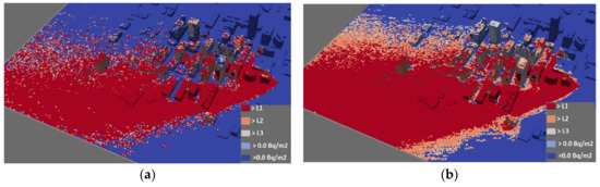
Figure 6.
Example of deposit on terrain for the model of Oklahoma City. (a) The figure corresponds to the run with 100,000 particles, and (b) the figure for 1,000,000 particles. The surfaces impacted by deposition are displayed using the categorization of L1, L2, L3 and non-zero.
The maximum value (=Dmax) is in all three cases the same, fluctuating by 2–3%. The area of the region with deposits above the level L1 (=10−3 × Dmax) changes by less than 1% from 106 to 5 × 10⁶, and by 10% from 105 to 106. The area of the region with deposits above the level L2 (=10−4 × Dmax) changes by about 2% from 106 to 5 × 10⁶, and by 16% from 105 to 106. Finally, the area of the region with deposits above the level L3 (=10−5 × Dmax) changes by about 7% from 106 to 5 × 10⁶, and by 24% from 105 to 106.
Applying about 1,000,000 particles reduces the statistical error of the main parameters that were modeled by 1–2%. The results were obtained within the approximate time of 10 min. The conclusion is that the implemented LPM is generally applicable in an emergency response in which results are required in short time periods.
The second part of the simulation is the radiological impact calculation. In the case of the computational domain of Kosice, we evaluated the three primary effects of the dose on the affected population. We tested two possible computing configurations (CPU and GPGPU), the same as for the dispersion analyses described above.
The radiological impact calculation has a different scale dependence than the dispersion calculation. In the radiological impact calculation, the computational time depends only on the number of cells (mainly in horizontal directions) or the number of cell surfaces; in other words, the computational time depends on the domain characteristics and not on the number particles. In our implemented computational approach for cloud shine (the ground shine and inhalation doses do not require such a technique), we work with an approximation in which the cells are grouped into larger supercells forming from one central cell and neighbors or even next-to-neighbors. These various levels of grouping are performed when the cells are beyond specified distances from the impacted point to minimize the approximation error. Therefore, the larger computational domain of Oklahoma City has approximately two times longer performance times for radiological impacts. We always consider buildings’ shielding effect, as described in Section 2.2 (Modelling of Radiological Effects).
The resulting performance is summarized in Table 6. For both configurations, we obtained a similar result. The whole calculation lasted less than 30 s. The radiological impacts are relevant only in a few time intervals after the event (e.g., 1 min, 3 min and 5 min and 10 min after the event). Therefore, the computational time for radiological impacts is low: 2 or 3 min in total. We can conclude analogously that the radiological impact calculation for dispersion is performed in real-time.
Table 6.
Time performance in seconds of radiological impact calculations for the model of Košice.
4. Conclusions and Summary
In this study, we implemented a Lagrangian particle model in the nuclear decision support system ESTE CBRN. The LPM is based on Thomson’s solution to the nonstationary, three-dimensional Langevin equation model for turbulent diffusion [7].
The validation was performed in two experimental environments. First, we modeled the cloud dispersion resulting from a continuous release, which is well described by Briggs sigma functions. In this comparison, a quasi-urban test field was modeled because the effect of buildings was included only implicitly in the vertical wind profiles. These wind profiles define the wind and turbulence fields in the entire computational domain without the actual buildings. Thus, this approach is more of a consistency test than a real validation. In this test case, we showed that the Briggs sigma functions are reproduced through LPM calculation satisfactorily. That means that the vertical wind profiles with high surface roughness corresponding to the presence of large buildings lead to a plume behavior similar to the urban Briggs sigma functions. Analogously, the profiles with low surface roughness lead to downwind dependence similar to that shown by Briggs sigma functions for rural conditions.
The implemented LPM was compared to the Joint Urban 2003 Street Canyon Experiment for instantaneous puff releases. This comparison setup represents an objective validation approach. We calculated the hourly mean wind fields for two IOPs, and we performed a comparison of the modeled atmospheric dispersion to mean behavior over three realized releases during the specific hour. We compared the maximum concentrations and peak times measured during two intensive operational periods of the JU2003 Experiment, IOP 3 and IOP 5. The modeled peak times are mostly 10 to 20% smaller than the measured ones. The maximum concentrations are reproduced moderately. The best modeled results were obtained when the measurements were laid in the approximate path of the puffs. Less accurate results were at locations farther from the main puff transport area, which are generally difficult places for modelling. These values were usually underestimated by more than a factor of 2. Thus, under the conditions we applied in the presented comparison to JU2003, the results are in moderate and adequate agreement.
The main concern of the work was to build a system potentially applicable for crisis situations to perform urban atmospheric transport calculations and radiological impact calculations within strict time requirements. These requirements assume that the whole calculation will be performed with a speed similar to the time scale of real events. Therefore, the urban model created is based on a parallel computation technique whereby particles are modeled simultaneously. The whole system is created as an application running on GPU technology.
In the final comparison, we prepared several computational 3D models of urban areas. We studied the computational times of the atmospheric dispersion calculation and the radiological parameter calculations. The focus is on the calculation on a GPU, which enables the calculation to be performed using a single computer. We show that the computational time is at the level of minutes, which copes with the need for crisis management. At the same time, a sufficient number of particles is applied to obtain acceptably accurate results. In our implementation, with about 1,000,000 or more modeled particles applied, the errors of resulting parameters are at several per cent.
Similarly, we show that the radiological parameters can be calculated quickly, which again fully complies with the needs of crisis management. The most time-demanding part is the calculation of effective dose from airborne activity, which is defined computationally as the sum of contributions from domain cells, including the shielding effect of the building walls. We show that contributions of all exposure pathways can be calculated in tens of seconds. Overall, we demonstrated that the whole computation of atmospheric dispersion and radiological impacts on the urban environment can be performed using a powerful computer in a time scale equal to the time scale of the real event.
Author Contributions
Conceptualization, Ľ.L., P.Č., E.F., M.M. (Michal Marčišovský), M.M. (Mária Marčišovská), M.C.; methodology, Ľ.L., P.Č., M.M. (Michal Marčišovský); software, Ľ.L., M.C.; validation, Ľ.L., P.Č., E.F.; formal analysis, Ľ.L., P.Č., E.F., M.M. (Michal Marčišovský), M.M. (Mária Marčišovská); investigation, Ľ.L., P.Č., E.F., M.M. (Michal Marčišovský), M.M. (Mária Marčišovská); resources, Ľ.L., P.Č., E.F., M.M. (Michal Marčišovský), M.M. (Mária Marčišovská); writing—original draft preparation, Ľ.L., P.Č., E.F., M.M. (Michal Marčišovský), M.M. (Mária Marčišovská); visualization, Ľ.L., E.F., M.C.; supervision, Ľ.L., P.Č., E.F., M.M. (Michal Marčišovský), M.M. (Mária Marčišovská); All authors have read and agreed to the published version of the manuscript.
Funding
This research was funded by Slovak Research and Development Agency (The Ministry of Education, Science, Research and Sport of the Slovak Republic), grant number APVV-20-0628. The research was co-funded also from internal resources of the company ABmerit, Ltd., where the authors are employed.
Institutional Review Board Statement
Not applicable.
Informed Consent Statement
Not applicable.
Data Availability Statement
The data of this analysis are publicly not available.
Conflicts of Interest
The authors declare no conflict of interest.
References
- Sykes, R.I.; Parker, S.F.; Henn, D.S.; Cerasoli, C.P.; Santos, L.P. PC-SCIPUFF Version 1.3—Technical Documentation; ARAP Report No. 725; Titan Corporation: San Diego, CA, USA, 2000. [Google Scholar]
- Briggs, G.A. Diffuion Estimation for Small Emissions, ATDL Contribution File No. 79; Atmospheric Turbulence and Diffusion Laboratory: Oak Ridge, TN, USA, 1973. [Google Scholar]
- Hanna, S.R.; Briggs, G.A.; Hosker, R.P. Handbook on Atmospheric Diffusion; Technical Report DOE-TIC-11223; Office of Energy Research, US Department of Energy: Washington, DC, USA, 1982.
- Liptak, L.; Fojcíková, E.; Carny, P. Comparison of the ESTE CBRN Model with the Joint Urban 2003 Experiment. Bound. Layer Meteorol. 2019, 171, 439–464. [Google Scholar] [CrossRef]
- Hernández-Ceballos, M.A.; Hanna, S.; Bianconi, R.; Bellasio, R.; Mazzola, T.; Chang, J.; Andronopoulos, S.; Armand, P.; Benbouta, N.; Čarný, P.; et al. UDINEE: Evaluation of Multiple Models with Data from the JU2003 Puff Releases in Oklahoma City. Part I: Comparison of Observed and Predicted Concentrations. Bound. Layer Meteorol. 2019, 171, 323–349. [Google Scholar] [CrossRef]
- Hernández-Ceballos, M.A.; Hanna, S.; Bianconi, R.; Bellasio, R.; Chang, J.; Mazzola, T.; Andronopoulos, S.; Armand, P.; Benbouta, N.; Čarný, P.; et al. UDINEE: Evaluation of Multiple Models with Data from the JU2003 Puff Releases in Oklahoma City. Part II: Simulation of Puff Parameters. Bound. Layer Meteorol. 2019, 171, 351–376. [Google Scholar] [CrossRef]
- Rodean, H.C. Stochastic Lagrangian Models of Turbulent Diffusion; The American Meteorological Society: Boston, MA, USA, 1996; 82p. [Google Scholar]
- Williams, M.D.; Brown, M.J.; Boswell, D.; Singh, B.; Pardyjak, E.M. Testing of the QUIC-Plume Model with Wind-Tunnel Measurements for a High-Rise Building. In Proceedings of the 26th Agricultural and Forest Meteorology/13th Air Pollution/5th Urban Environment/16th Biometeorology and Aerobiology, January 2004. Available online: https://ams.confex.com/ams/AFAPURBBIO/webprogram/Paper78636.html (accessed on 2 May 2023).
- Benbouta, N. Canadian Urban Flow and Dispersion Model (CUDM): Developing Canadian Capabilities for CBRN Hazard Dispersion in Urban Areas; CMOE Dorval TR 2007-001 Technical Report; Environment Canada: Toronto, ON, Canada, 2007. [Google Scholar]
- Hogue, R.; Benbouta, N.; Mailhot, J.; Belair, S.; Lemonsu, A.; Yee, E.; Lien, F.-S.; Wilson, J.D. The development of a prototype of Canadian urban flow and dispersion modeling system. In Proceedings of the AMS 89 Annual Conference, Joint Session 19 Urban Transport and Dispersion Modeling, Phoenix, AZ, USA, 14 January 2009. [Google Scholar]
- Oldrini, O.; Armand, P.; Duchenne, C.; Olry, C.; Moussafir, J.; Tinarelli, G. Description and preliminary validation of the PMSS fast response parallel atmospheric flow and dispersion solver in complex built-up areas. Environ. Fluid Mech. 2017, 17, 997–1014. [Google Scholar] [CrossRef]
- Oldrini, O.; Armand, P.; Duchenne, C.; Perdriel, S. Parallelization Performances of PMSS Flow and Dispersion Modeling System over a Huge Urban Area. Atmosphere 2019, 10, 404. [Google Scholar] [CrossRef]
- Röckle, R. Bestimmung der Strömungsverhältnisse im Bereich komplexer Bebauungsstrukturen. Ph.D. Thesis, Techn. Hochschule Darmstadt, Darmstadt, Germany, 1990. [Google Scholar]
- Ek, N.; Benbouta, N.; Bourgouin, P.; Gauthier, J.-P.; Gauthier, N.; Hogue, R.; Holly, M.; Trudel, S.; Zaganescu, C. The Canadian urban dispersion modelling (CUDM) system: An operational prototype. In Proceedings of the 34th AMOP Technical Seminar on Environmental Contamination and Response, Banff, AB, Canada, 4–6 October 2011; pp. 603–623. [Google Scholar]
- Thomson, D.J. Criteria for the selection of stochastic models of particle trajectories in turbulent flows. J. Fluid Mech. 1987, 180, 529–556. [Google Scholar] [CrossRef]
- Patankar, S.V.; Spalding, D.B. A calculation procedure for heat, mass and momentum transfer in three-dimensional parabolic flows. Int. J. Heat Mass Transf. 1972, 15, 1787–1806. [Google Scholar] [CrossRef]
- Roed, J.; Andersson, K.G. Early Measurements in Scandinavia following the Chernobyl Accident (IAEA-TECDOC—1131); International Atomic Energy Agency (IAEA): Vienna, Austria, 2000. [Google Scholar]
- Lipták, Ľ.; Fojcíková, E.; Krpelanová, M.; Fabová, V.; Čarný, P. The ESTE Decision Support System for Nuclear and Radiological Emergencies: Atmospheric Dispersion Models. Atmosphere 2021, 12, 204. [Google Scholar] [CrossRef]
- ParaView—Open Source Post-Processing Visualization Engine. Available online: https://www.paraview.org/ (accessed on 25 June 2023).
- Clawson, K.L.; Carter, R.G.; Lacroix, D.J.; Biltoft, C.A.; Hukari, N.F.; Johnson, R.C.; Rich, J.D. Joint Urban 2003 (JU03) SF6 Atmospheric Tracer Field Tests; NOAA Technical Memorandum OARARL-254; Air Resources Lab.: College Park, MD, USA, 2005. [Google Scholar]
- Allwine, K.J.; Leach, M.J.; Stockham, L.W.; Shinn, J.S.; Hosker, R.P.; Bowers, J.F.; Pace, J.C. Overview of Joint Urban 2003—An atmospheric Dispersion Study in Oklahoma City. Preprints, Symposium on Planning, Nowcasting and Forecasting in the Urban Zone, American Meteorological Society. 2004. Available online: www.researchgate.net (accessed on 23 June 2023).
- Wesson, G.; Katul, G.; Lai, C.-T. Sensible heat flux estimation by flux variance and half-order time derivative methods. Water Resour. Res. 2001, 37, 2333–2343. [Google Scholar] [CrossRef]
- Möller, T.; Trumbore, B. Fast, Minimum Storage Ray-Triangle Intersection. J. Graph. Tools 1997, 2, 21–28. [Google Scholar] [CrossRef]
- Los Alamos National Laboratory. MCNP—A General Monte Carlo N-Particle Transport Code, Version 5, Software Product Produced by Los Alamos National Laboratory. Available online: https://mcnp.lanl.gov/ (accessed on 2 February 2021).


Disclaimer/Publisher’s Note: The statements, opinions and data contained in all publications are solely those of the individual author(s) and contributor(s) and not of MDPI and/or the editor(s). MDPI and/or the editor(s) disclaim responsibility for any injury to people or property resulting from any ideas, methods, instructions or products referred to in the content. |
© 2023 by the authors. Licensee MDPI, Basel, Switzerland. This article is an open access article distributed under the terms and conditions of the Creative Commons Attribution (CC BY) license (https://creativecommons.org/licenses/by/4.0/).