

Using Machine Learning to Predict Wind Flow in Urban Areas

Abstract
1. Introduction
2. Materials and Methods
2.1. RANS Model
2.2. Machine Learning
2.3. Test Cases
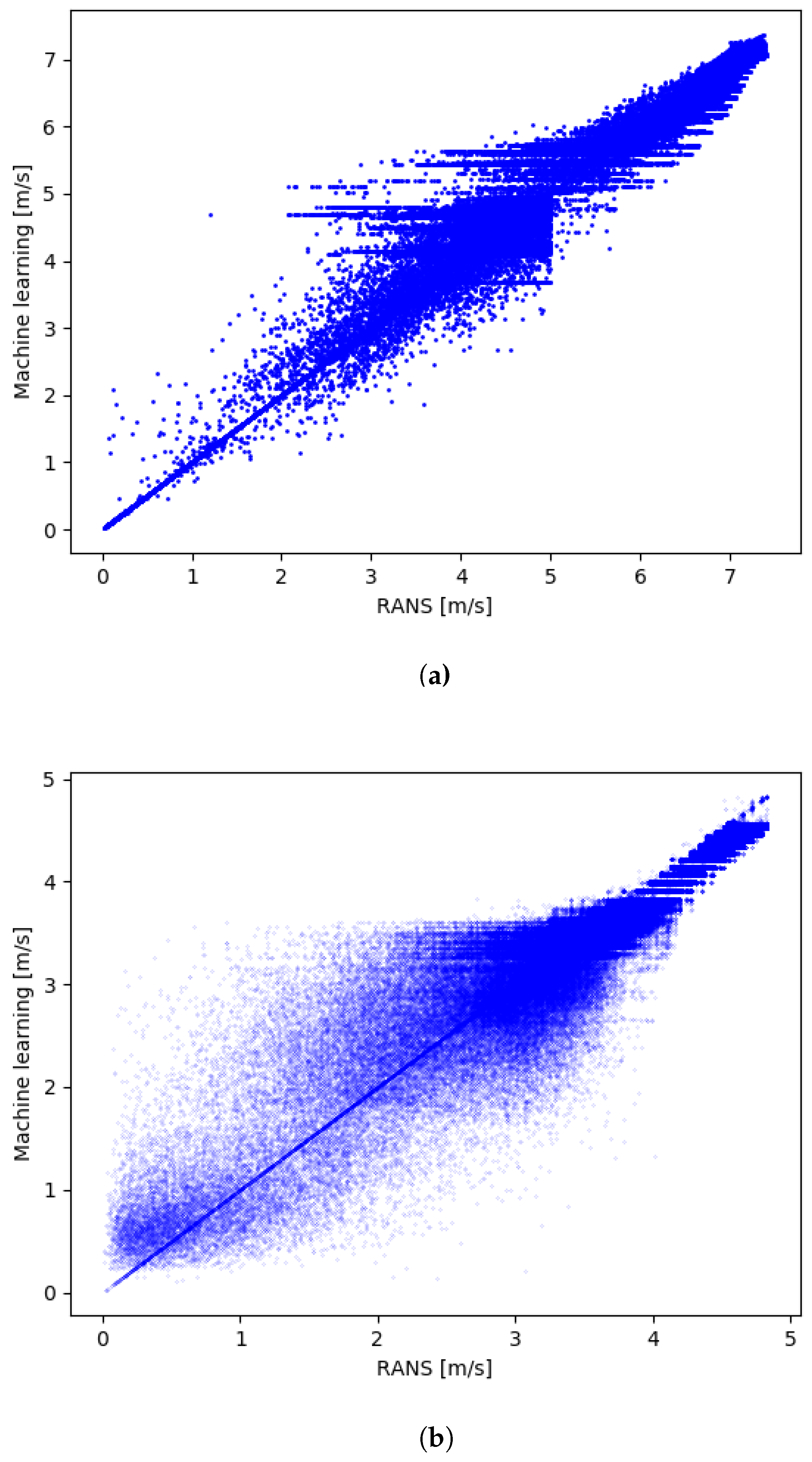
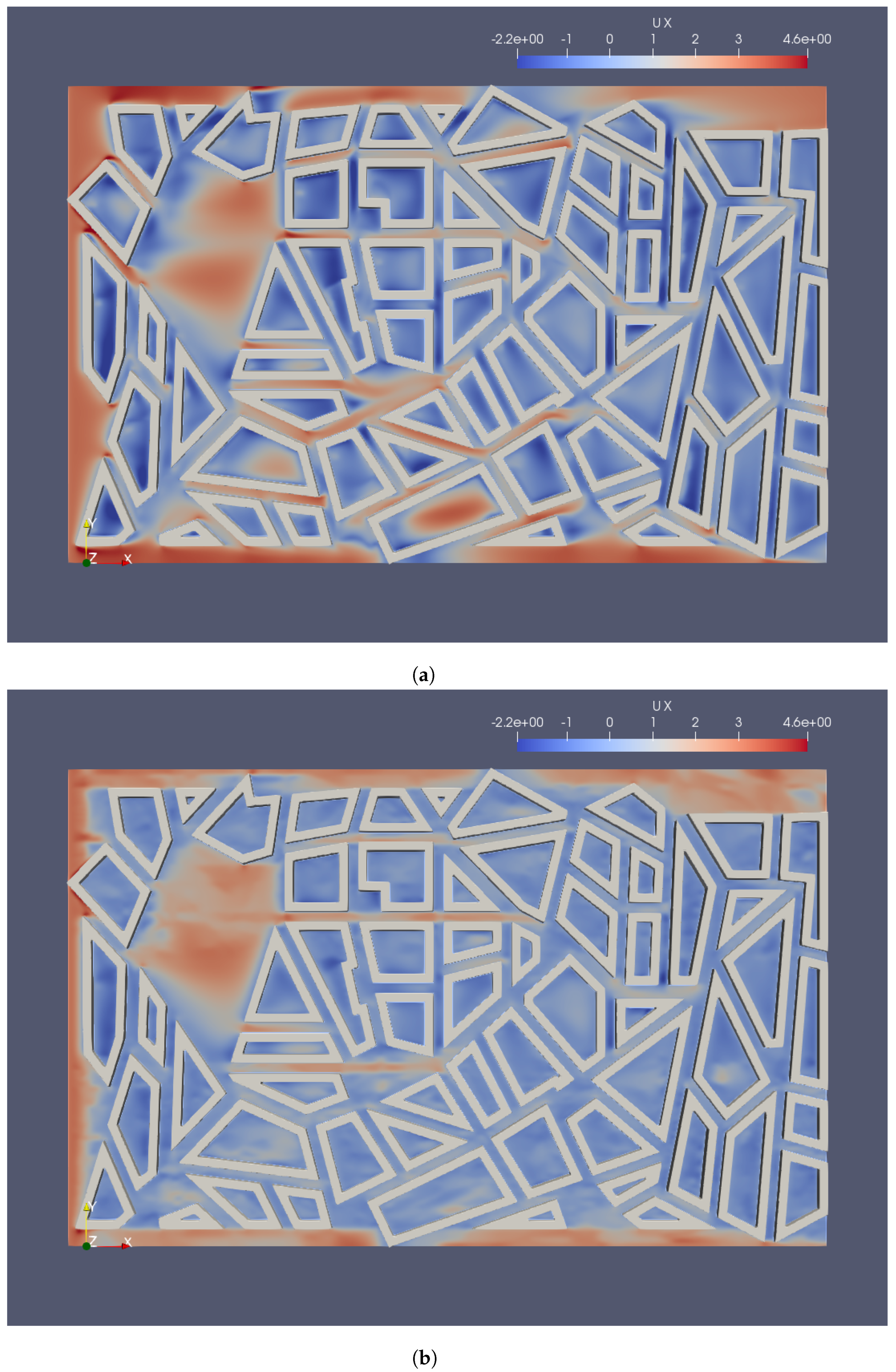
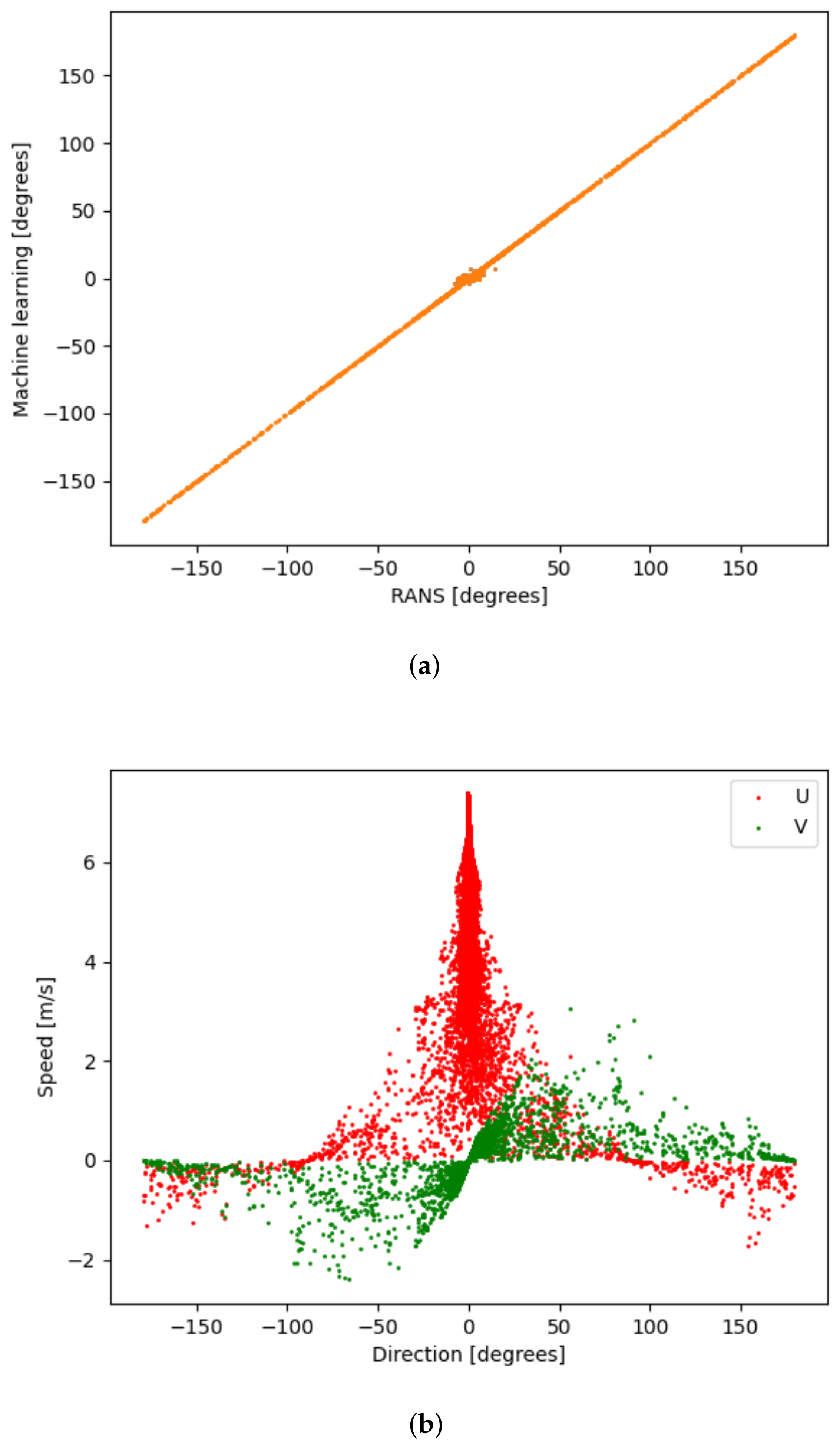
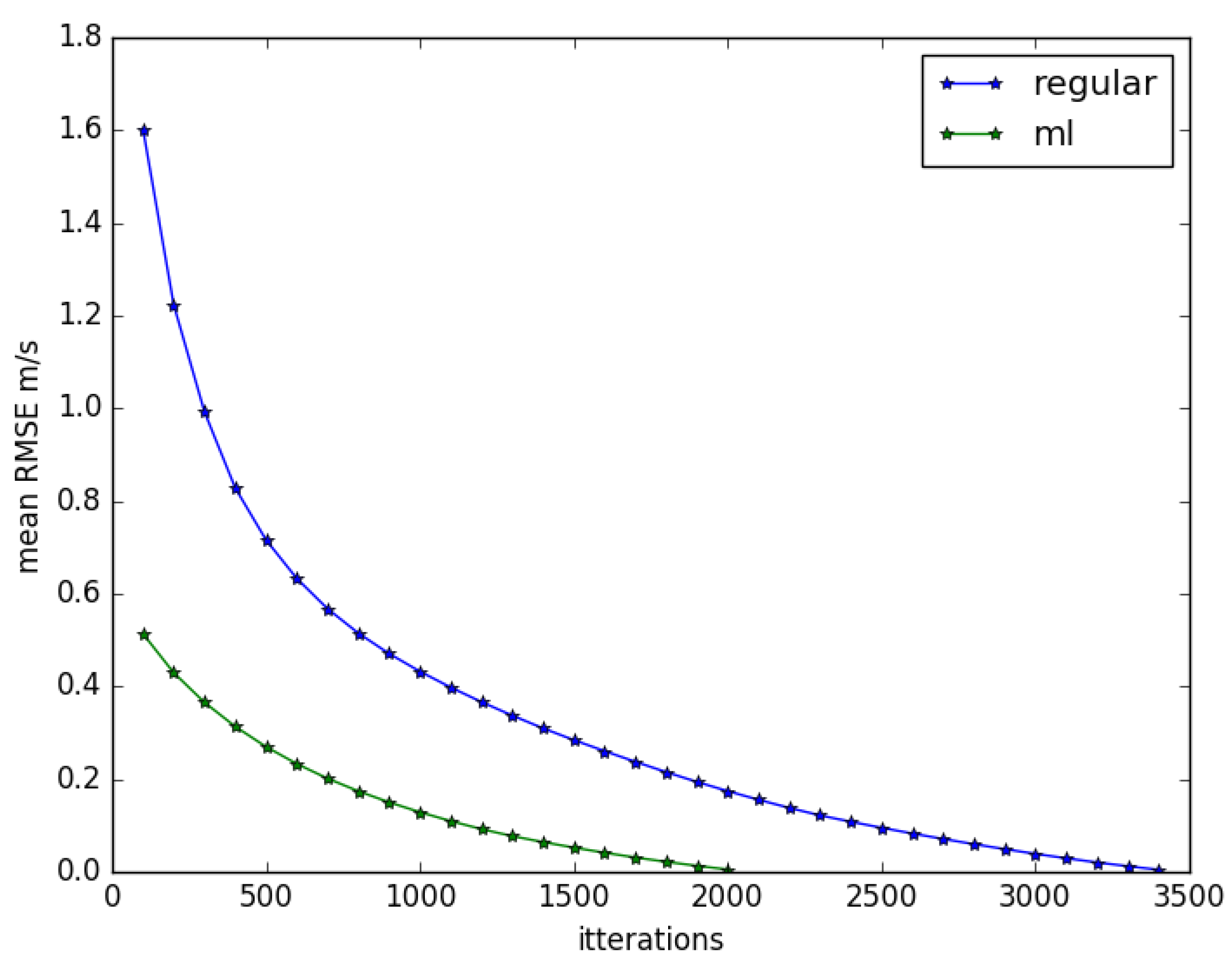
3. Results
4. Discussion and Conclusions
Author Contributions
Funding
Acknowledgments
Conflicts of Interest
Abbreviations
| kNN | k Nearest Neighbors |
| ML | Machine learning |
| RANS | Reynolds-Averaged Navier–Stokes |
| WT | Wind Tunnel |
References
- Hanna, S.R.; Brown, M.J.; Camelli, F.E.; Chan, S.T.; Coirier, W.J.; Hansen, O.R.; Huber, A.H.; Kim, S.; Reynolds, R.M. Detailed simulations of atmospheric flow and dispersion in downtown Manhattan: An application of five computational fluid dynamics models. Bull. Am. Meteorol. Soc. 2006, 87, 1713–1726. [Google Scholar] [CrossRef]
- Gromke, C.; Buccolieri, R.; Di Sabatino, S.; Ruck, B. Dispersion study in a street canyon with tree planting by means of wind tunnel and numerical investigations—Evaluation of CFD data with experimental data. Atmos. Environ. 2008, 42, 8640–8650. [Google Scholar] [CrossRef]
- Spirn, A. Better Air Quality at Street Level: Strategies for Urban Design. In Public Streets for Public Use; Van Nostrand Reinhold: New York, NY, USA, 1987. [Google Scholar]
- Cheng, W.C.; Yang, Y. Scaling of Flows Over Realistic Urban Geometries: A Large-Eddy Simulation Study. Bound. Layer Meteorol. 2022, 186, 125–144. [Google Scholar] [CrossRef]
- Blocken, B.; Persoon, J. Pedestrian wind comfort around a large football stadium in an urban environment: CFD simulation, validation and application of the new Dutch wind nuisance standard. J. Wind. Eng. Ind. Aerodyn. 2009, 97, 255–270. [Google Scholar] [CrossRef]
- Moonen, P.; Defraeye, T.; Dorer, V.; Blocken, B.; Carmeliet, J. Urban Physics: Effect of the micro-climate on comfort, health and energy demand. Front. Archit. Res. 2012, 1, 197–228. [Google Scholar] [CrossRef]
- Neophytou, M.; Gowardhan, A.; Brown, M. An inter-comparison of three urban wind models using Oklahoma City Joint Urban 2003 wind field measurements. J. Wind. Eng. Ind. Aerodyn. 2011, 99, 357–368. [Google Scholar] [CrossRef]
- Tominaga, Y.; Stathopoulos, T. Numerical simulation of dispersion around an isolated cubic building: Model evaluation of RANS and LES. Build. Environ. 2010, 45, 2231–2239. [Google Scholar] [CrossRef]
- Blocken, B.; Stathopoulos, T.; Van Beeck, J. Pedestrian-level wind conditions around buildings: Review of wind-tunnel and CFD techniques and their accuracy for wind comfort assessment. Build. Environ. 2016, 100, 50–81. [Google Scholar] [CrossRef]
- Nimarshana, P.; Attalage, R.; Perera, K.K.C. Quantification of the impact of RANS turbulence models on airflow distribution in horizontal planes of a generic building under cross-ventilation for prediction of indoor thermal comfort. J. Build. Eng. 2022, 52, 104409. [Google Scholar] [CrossRef]
- Anup, K.; Whale, J.; Urmee, T. Urban wind conditions and small wind turbines in the built environment: A review. Renew. Energy 2019, 131, 268–283. [Google Scholar]
- Toja-Silva, F.; Kono, T.; Peralta, C.; Lopez-Garcia, O.; Chen, J. A review of computational fluid dynamics (CFD) simulations of the wind flow around buildings for urban wind energy exploitation. J. Wind. Eng. Ind. Aerodyn. 2018, 180, 66–87. [Google Scholar] [CrossRef]
- Jordan, M.I.; Mitchell, T.M. Machine learning: Trends, perspectives, and prospects. Science 2015, 349, 255–260. [Google Scholar] [CrossRef]
- Mahesh, B. Machine learning algorithms—A review. Int. J. Sci. Res. 2020, 9, 381–386. [Google Scholar]
- Zhao, Y.; Akolekar, H.D.; Weatheritt, J.; Michelassi, V.; Sandberg, R.D. RANS turbulence model development using CFD-driven machine learning. J. Comput. Phys. 2020, 411, 109413. [Google Scholar] [CrossRef]
- Wu, J.L.; Xiao, H.; Paterson, E. Physics-informed machine learning approach for augmenting turbulence models: A comprehensive framework. Phys. Rev. Fluids 2018, 7, 1–42. [Google Scholar] [CrossRef]
- Maulik, R.; Sharma, H.; Patel, S.; Lusch, B.; Jennings, E. Accelerating RANS Turbulence Modeling Using Potential Flow and Machine Learning. arXiv 2019, arXiv:1910.10878. [Google Scholar]
- Vuppala, R.K.; Kara, K. A non-intrusive reduced order model using deep learning for realistic wind data generation for small unmanned aerial systems in urban spaces. AIP Adv. 2022, 12, 085020. [Google Scholar] [CrossRef]
- Mortezazadeh, M.; Zou, J.; Hosseini, M.; Yang, S.; Wang, L. Estimating Urban Wind Speeds and Wind Power Potentials Based on Machine Learning with City Fast Fluid Dynamics Training Data. Atmosphere 2022, 13, 214. [Google Scholar] [CrossRef]
- Altman, N.S. An introduction to kernel and nearest-neighbor nonparametric regression. Am. Stat. 1992, 46, 175–185. [Google Scholar] [CrossRef]
- Chrit, M.; Majdi, M. Improving Wind Speed Forecasting for Urban Air Mobility Using Coupled Simulations. Adv. Meteorol. 2022, 2022, 2629432. [Google Scholar] [CrossRef]
- Chrit, M. Reconstructing urban wind flows for urban air mobility using reduced-order data assimilation. Theor. Appl. Mech. Lett. 2023, 13, 100451. [Google Scholar] [CrossRef]
- Baumann-Stanzer, K.; Andronopoulos, S.; Armand, P.; Berbekar, E.; Efthimiou, G.; Fuka, V.; Gariazzo, C.; Gasparac, G.; Harms, F.; Hellsten, A.; et al. COST ES1006 Model Evaluation. 2015. Available online: https://www.researchgate.net/publication/275952924_COST_ES1006_Model_evaluation_case_studies_Approach_and_results (accessed on 17 January 2023).
- Reynolds, O. On the Dynamical Theory of Incompressible Viscous Fluids and the Determination of the Criterion. Philos. Trans. R. Soc. Lond. 1895, 186, 123–164. [Google Scholar]
- Menter, F.R. Improved Two-Equation k–Omega Turbulence Models for Aerodynamic Flows—NASA Technical Memorandum TM-103975; NASA Technical Memorandum NASA; NASA Ames Research Center: Moffett Field, CA, USA, 1992; pp. 1–31. [Google Scholar]
- Caretto, L.S.; Gosman, A.D.; Patankar, S.V.; Spalding, D.B. Two Calculation Procedures for Steady, Three-Dimensional Flows with Recirculation. In Proceedings of the Third International Conference on Numerical Methods in Fluid Mechanics; Springer: Cham, Switzerland, 2004; pp. 60–68. [Google Scholar] [CrossRef]
- Churchfield, M.J.; Moriarty, P.J.; Vijayakumar, G.; Brasseur, J.G. Wind Energy-Related Atmospheric Boundary Layer Large-Eddy Simulation Using OpenFOAM. In Proceedings of the 19th Symposium on Boundary Layers and Turbulence, Keystone, CO, USA, 2–6 August 2010; pp. 1–26. [Google Scholar]
- Soomro, A.A.; Mokhtar, A.A.; Salilew, W.M.; Abdul Karim, Z.A.; Abbasi, A.; Lashari, N.; Jameel, S.M. Machine Learning Approach to Predict the Performance of a Stratified Thermal Energy Storage Tank at a District Cooling Plant Using Sensor Data. Sensors 2022, 22, 7687. [Google Scholar] [CrossRef]
- Pedregosa, F.; Varoquaux, G.; Gramfort, A.; Michel, V.; Thirion, B.; Grisel, O.; Blondel, M.; Prettenhofer, P.; Weiss, R.; Dubourg, V.; et al. Scikit-learn: Machine Learning in Python. J. Mach. Learn. Res. 2011, 12, 2825–2830. [Google Scholar]
- Oke, T.R. Street design and urban canopy layer climate. Energy Build. 1988, 11, 103–113. [Google Scholar] [CrossRef]
- Vardoulakis, S.; Fisher, B.E.; Pericleous, K.; Gonzalez-Flesca, N. Modelling air quality in street canyons: A review. Atmos. Environ. 2003, 37, 155–182. [Google Scholar] [CrossRef]
- Rakai, A.; Franke, J. Validation of two RANS solvers with flow data of the flat roof Michelstadt case. Urban Clim. 2014, 10, 758–768. [Google Scholar] [CrossRef]
- Efthimiou, G.C.; Bartzis, J.G.; Berbekar, E.; Hertwig, D.; Harms, F.; Leitl, B. Modelling short-term maximum individual exposure from airborne hazardous releases in urban environments. Part II: Validation of a deterministic model with wind tunnel experimental data. Toxics 2015, 3, 259–267. [Google Scholar] [CrossRef]
- Efthimiou, G.C.; Kovalets, I.V.; Argyropoulos, C.D.; Venetsanos, A.; Andronopoulos, S.; Kakosimos, K.E. Evaluation of an inverse modelling methodology for the prediction of a stationary point pollutant source in complex urban environments. Build. Environ. 2018, 143, 107–119. [Google Scholar] [CrossRef]
- Castelli, S.T.; Armand, P.; Tinarelli, G.; Duchenne, C.; Nibart, M. Validation of a Lagrangian particle dispersion model with wind tunnel and field experiments in urban environment. Atmos. Environ. 2018, 193, 273–289. [Google Scholar] [CrossRef]
- Knapp, T.R. Canonical correlation analysis: A general parametric significance-testing system. Psychol. Bull. 1978, 85, 410–416. [Google Scholar] [CrossRef]
- Chang, J.C.; Hanna, S.R. Air quality model performance evaluation. Meteorol. Atmos. Phys. 2004, 87, 167–196. [Google Scholar] [CrossRef]


| Index | RANS | ML |
|---|---|---|
| CCA | 0.96 | 0.93 |
| r | 0.93 | 0.90 |
| Factor 2 | 0.84 | 0.65 |
| RMSD m/s | 0.67 | 0.87 |
| Observation Mean m/s | 2.47 | 2.47 |
| Model Mean m/s | 2.11 | 2.08 |
| Observation STD m/s | 1.52 | 1.52 |
| Model STD m/s | 1.52 | 1.79 |
| Coarse | Medium | Fine | |
|---|---|---|---|
| number of cells | 0.5 M | 2.5 M | 9.5 M |
| simulation duration [h] | 0.1 | 0.9 | 7.3 |
| RMSD (vs. Observation) | 0.494 | 0.483 | 0.472 |
| Feature | Set I | Set II | Set III |
|---|---|---|---|
| Distance from ground | 1.90 | 2.01 | 2.66 |
| mean height (including buildings) | - | 0 | 0 |
| distance from next building in direction | 1.047 | 0.873 | 1.61 |
| distance from previous building in direction | 1.961 | 1.946 | 1.77 |
| street width in direction | - | 0.187 | 0 |
| street width in direction | - | 0.709 | 0 |
| distance from building in left in direction | 0.589 | 0.259 | 1.51 |
| distance from building in right in direction | 0.413 | 0 | 0.98 |
| height of the previous building in direction | 0.321 | 0.097 | −0.01 |
| height of the following building in direction | 0.176 | 0.053 | 0.01 |
| street angle | - | - | −2.54 |
| ratio between the distance from the previous building and the previous building height | - | - | −0.02 |
| ratio between the distance from the following building and the following building height | - | - | 0.05 |
Disclaimer/Publisher’s Note: The statements, opinions and data contained in all publications are solely those of the individual author(s) and contributor(s) and not of MDPI and/or the editor(s). MDPI and/or the editor(s) disclaim responsibility for any injury to people or property resulting from any ideas, methods, instructions or products referred to in the content. |
© 2023 by the authors. Licensee MDPI, Basel, Switzerland. This article is an open access article distributed under the terms and conditions of the Creative Commons Attribution (CC BY) license (https://creativecommons.org/licenses/by/4.0/).
Share and Cite
BenMoshe, N.; Fattal, E.; Leitl, B.; Arav, Y. Using Machine Learning to Predict Wind Flow in Urban Areas. Atmosphere 2023, 14, 990. https://doi.org/10.3390/atmos14060990
BenMoshe N, Fattal E, Leitl B, Arav Y. Using Machine Learning to Predict Wind Flow in Urban Areas. Atmosphere. 2023; 14(6):990. https://doi.org/10.3390/atmos14060990
Chicago/Turabian StyleBenMoshe, Nir, Eyal Fattal, Bernd Leitl, and Yehuda Arav. 2023. "Using Machine Learning to Predict Wind Flow in Urban Areas" Atmosphere 14, no. 6: 990. https://doi.org/10.3390/atmos14060990
APA StyleBenMoshe, N., Fattal, E., Leitl, B., & Arav, Y. (2023). Using Machine Learning to Predict Wind Flow in Urban Areas. Atmosphere, 14(6), 990. https://doi.org/10.3390/atmos14060990