Spatiotemporal Heterogeneity of Temperature and Precipitation in Complex Terrain along the Northeastern Margin of the Tibetan Plateau

Abstract

The study of climate element distribution models under complex terrain conditions is a popular topic in the field of GIS application in climatology, especially in plateau areas with a complex topography and scarce meteorological station information. In this paper, the spatial and temporal heterogeneity of temperature and precipitation at the northeastern edge of the Tibetan Plateau was analyzed by taking the northeastern edge of the plateau as the study area and constructing a topographic spatial statistical model using 47 meteorological stations and digital elevation models from 1981 to 2010. The following conclusions were drawn from the study: (1) The ME of the temperature distribution model for each month is below 0.9 °C; the maximum ME of the precipitation distribution model for each month is −5.808 mm in July, and the precipitation distribution model has similar error characteristics with the temperature distribution model, which can reflect the horizontal zone distribution pattern of meteorological data and can clearly show the changes of temperature and precipitation as the altitude increases. (2) The spatial distribution pattern of temperature is as follows: the temperature in the study area gradually increases from the southwest to the northeast, with Zhouqu County in Linxia Prefecture and Gannan Prefecture as the main high-temperature areas; the spatial distribution of precipitation is as follows: the precipitation in the southwest of the study area is significantly higher than that in the north, and the precipitation in Linxia Prefecture is significantly lower than that in Gannan Prefecture. (3) The temporal distribution pattern of the temperature distribution model is as follows: the overall temperature in the study area is at its lowest level in January, and the maximum temperature is only 2.6 °C, until July, when the maximum temperature rises to 24.2 °C and then gradually starts to decline; the spatial distribution of precipitation is as follows: the precipitation in the study area gradually rises from January, and the maximum precipitation rises to July and then starts to decline, and in December the precipitation falls to the lowest level. The temporal distribution characteristics of the precipitation distribution model are similar to those of the air temperature model, with obvious hydrothermal synchronization characteristics.

1. Introduction

The application performance of traditional geostatistical methods depends to a large extent on the spatial density of the samples and rarely considers the spatial evolution or mechanism characteristics of the analyzed elements [1,2]. The complex topographic characteristics of alpine regions make it difficult for traditional spatial analyses to meet the requirements of complex climate spatial distribution studies. In practice, the number of weather stations is very limited due to the constraints of topography and human and financial resources. Especially in complex terrain, the limited observation data cannot accurately express the overall spatial and temporal distribution of meteorological elements [3,4,5,6], and the conventional spatial interpolation methods cannot reflect the spatial variability characteristics of meteorological elements with topographic changes [7,8,9]. Xin Li [10] pointed out the need to select the best interpolation method according to the actual environmental characteristics. In the complex region of the study area where the native ecological environment is fragile and increasingly degraded under the interacting stress of global environmental changes and human activities, it is urgent to analyze the spatial and temporal characteristics of its climate elements at a finer scale and more accurately; however, there are very few studies on the northeastern edge of the Qinghai-Tibet Plateau, and it is important and necessary to advance ecological research in the study area [11].

Spatial interpolation is the most widely used method for the spatial extrapolation of climate elements in the object area from station observations, and there are many methods used to estimate the spatial distribution of regional surface precipitation and temperature, and they are more frequently applied to the attribute elements of meteorological data [12,13,14,15,16,17,18]. In recent years, with the development of GIS and remote sensing providing a large amount of real and reliable data as well as powerful spatial analysis techniques, scholars around the world have applied a series of interpolation methods to study the distribution of climate elements [19,20,21,22,23,24,25,26,27]. Ashraf et al. [26] used the inverse distance-squared weighting method, inverse distance weighting (IDW) method, ordinary kriging and cokriging methods to estimate the distribution of climate elements in Nebraska and Kansas. The RMSE ranking found that cokriging distributed climate elements more accurately than the distance inverse. Price et al. [7] interpolated 30-year monthly mean maximum and minimum temperature and rainfall data for western and eastern Canada using the thin-slab smooth spline and gradient distance inverse square methods, and by comparing the root-mean-square error and the thin-slab smooth spline, Lu et al. [27] addressed the shortcomings of the inverse distance weighting method, which has the same power exponent throughout the study area, and pointed out that the sample point aggregation area should be assigned a smaller power exponent, and the improved inverse distance weighting method is better than the inverse distance weighting method with a constant power exponent. Nalder [28] studied four forms of kriging and three simple alternatives to estimate 30-year means (normal values) of monthly temperature and precipitation at specific locations in western Canada and found that the GIDS method, which introduces elevation, was more appropriate for his study area. Goovaerts [29] confirmed that the interpolation method outperformed the rest of the interpolation methods using annual and monthly precipitation data measured at 36 climate stations for a 5000 km² area in Portugal and incorporating digital elevation models into three multivariate geostatistical calculations for spatial predictions.

Bi et al. [22] applied the Tyson polygon method in the estimation of average rainfall in the Haihe River basin to better reflect the actual local precipitation distribution, but the method resulted in the same amount of precipitation everywhere within the polygon and abrupt changes in the amount of precipitation between the polygons due to the point-by-point approach. Although Liang [23] used the inverse distance weighting method to improve the accuracy and computational efficiency of surface rainfall estimation in the Huaihe River basin and subbasins, this method relies heavily on the number of known points and is influenced by extreme values. Li [24] applied the kriging method to interpolate precipitation in some areas of the Wuding River basin to obtain more acceptable results. Most of the abovementioned study areas are located in areas with little elevation variability and relatively flat topography and are large-scale studies. Spatial interpolation only considers the spatial location, which cannot truly reflect the local variation in precipitation in mountainous areas with complex topography. The ecological functioning of the upper reaches of the Yellow River in the study area is sensitive to ecological changes and has a pivotal ecological status. The increasing deterioration of the ecological environment is directly related to the ecological security of the Yangtze and Yellow River basins and the sustainable development of the economy and society, and while an increasing number of scholars are studying the temperature, precipitation and ecological aspects of the study area [30,31,32], there are few studies on the distribution of fine-scale meteorological elements in the study area.

The purpose of this study is to analyze the spatial and temporal characteristics of temperature and precipitation in the study area. Specifically, the objectives of this study are as follows: (1) to construct a temperature and precipitation distribution model applicable to the alpine and complex topographic features of the study area; (2) to construct a monthly temperature and precipitation dataset of the study area from 1980 to 2010; and (3) to explore the spatial and temporal distribution characteristics of temperature and precipitation in the study area.

2. Study Area

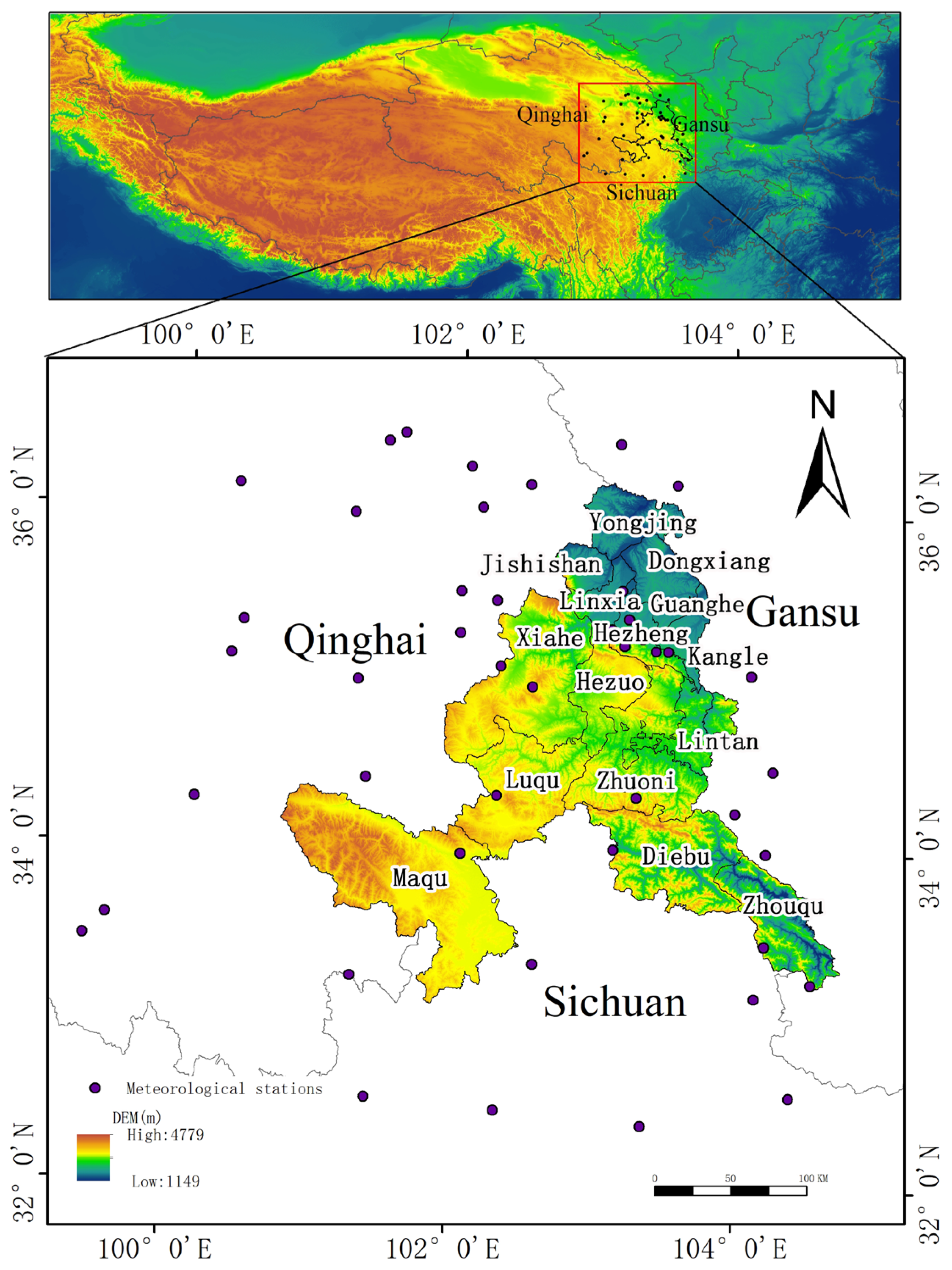
The study area is located on the northeastern edge of the Tibetan Plateau, which mainly includes the Gannan Tibetan Autonomous Prefecture and Linxia Hui Autonomous Prefecture (Figure 1). As an important component of the world’s Third Pole region, the study area is a uniquely coupled system of geology, geography, resources, ecology, and people [33] and an important fragile alpine ecological region. It not only has a significant impact on environmental climate change in the Yellow River basin and even northern China but is also sensitive to the impact of global environmental change and human activities [34].

The study area is located on the northeastern edge of the Tibetan Plateau, the transition zone from the first to the second step, and is where the Tibetan Plateau, the Loess Plateau, and the Sichuan Basin intersect. The region is located at the intersection of the Qinling and Kunlun trough fold systems, most of which belong to the Qinling trough fold system, while the southwestern part belongs to the Songpan-Ganzi trough fold system. The mountains and plateaus in the territory alternate, forming mountainous areas, mountain canyon areas, mountain hilly areas and other geomorphic types [35], with undulating terrain. The vegetation of the study area reflects the intersection of three plant subregions: China-Japan, China-Himalaya, and the Tibetan Plateau. The study area is an important area influenced by the seasonal autumn rain in western China and is an important part of the ecological barrier of the Tibetan Plateau. The Taohe and Daxia Rivers, important tributaries of the Yellow River, originate from the study area, and as an important water recharge area in the upper reaches of the Yellow River, the study area assumes an important water-retaining function, and its water storage and recharge function play a key role in the mobilization and regulation of water resources in the entire Yellow River basin [34].

The northeastern margin of the Qinghai-Tibet Plateau is very representative of autumn rainfall in western China, where the frequent southward cold front in autumn and the warm and humid air stagnating in western China intersect to intensify the frontal activity, thus producing long periods of clouds and rain [36,37,38,39,40]. Precipitation mainly occurs in September and October, and the amount of precipitation is generally higher than that in spring and also in summer, which is hydrologically significant as autumn flooding. The important tributaries of the Yellow River, Taohe and Daxia, originate from the northeast edge of the Qinghai-Tibet Plateau, and as an important water recharge area in the upper reaches of the Yellow River, the northeast edge of the Qinghai-Tibet Plateau assumes an important water-retaining function, and its water storage and recharge function plays a key role in the mobilization and regulation of water resources in the entire Yellow River basin [37]. The study of this area is of great importance because of its poor resistance to disturbances caused by both natural and human factors [41].

3. Data and Methods

The data to be used in this study are meteorological station observation data, geographic coordinate data of meteorological stations and a digital elevation model. All the obtained data are analyzed and entered using ArcGIS and used for the subsequent construction of spatial and temporal models of temperature and precipitation.

(1) Observational data from meteorological stations: The Monthly Value Dataset of China’s Terrestrial Climate Standard Values (1981–2010) was released by the China Meteorological Data Network (http://data.cma.cn/, accessed on 25 September 2021). This dataset is obtained from the national monthly value information data reported by provinces based on the statistics of the professional meteorological data compilation method, which has strong validity. The dataset includes 2160 ground meteorological observation stations in China, covering various meteorological elements such as temperature, air humidity, air pressure, precipitation and other meteorological elements. A total of 47 meteorological stations, including Gaolan Station, are used in this study, covering Gansu, Sichuan and Qinghai provinces.

(2) Digital elevation model: The geospatial data cloud (http://www.gscloud.cn/accounts/login_user accessed on 25 September 2021), product name: SRTMDEM 90 m, are jointly measured by NASA and NIMA; the quality is reliable, and the data cover more than 80% of the Earth’s land surface with a spatial resolution of 90 m.

(3) Precipitation product data: This dataset (https://data.tpdc.ac.cn/zh-hans/data/ accessed on 25 April 2023) is the month-by-month precipitation data of China with the spatial resolution of 0.0083333° (about 1 km) and the time of January 1901–December 2021. The data format is NETCDF, i.e., .nc format. The dataset is generated by the Delta spatial downscaling scheme in the Chinese region based on the global 0.5° climate dataset released by CRU and the global high-resolution climate dataset released by WorldClim. And the data from 496 independent meteorological observation points were used to validate the results with confidence. The geospatial scope of this dataset is the mainland area of the country (including Hong Kong, Macao and Taiwan), excluding areas such as islands and reefs in the South China Sea. The precipitation units are 0.1 mm.

3.1. Topographic Spatial Statistics Method

This study constructs a temperature and precipitation distribution model based on data from 47 ground stations and digital elevation models from 1981 to 2010, applicable to the alpine and complex topographic features of the study area, analyzes the geospatial statistical structure characteristics of the 30-year average monthly annual climate elements (temperature and precipitation) from 1981 to 2010 in detail using classical statistics, and analyzes the structural statistical laws of climate elements. To analyze the geospatial influence on the distribution of climate elements with geographic computational visualization techniques, we interpolate the residual spatial structure of climate elements with structural features removed to build a distributed climate model that can be represented by existing meteorological station data and create a temperature and precipitation distribution model that is suitable for simulating alpine and complex regions and can reflect their topographic features (Figure 2).

3.2. Statistical Analysis of Climate Elements

The structural patterns of climate elements and geographical three-dimensional space (longitude, dimension, altitude) are visualized and analyzed separately, and the structural model between a single geospatial factor and climate factors is determined. The three structural models are integrated to form a functional form that reflects the global structure of climate elements in the region.

In the structural model, longitude is used to represent the longitudinal variation in precipitation characteristics from the coastal to inland direction approximately in the east-west direction under the influence of sea-land distribution; latitude represents how the regional moisture conditions, water vapor transport and water phase change into a latitudinal band by determining the amount of solar radiation; and altitude affects the condensation height of water vapor by changing the heat condition of the ground, causing vertical variation in precipitation. At the same time, it redistributes the precipitation through the influence of water vapor blocking, which represents the difference in the spatial distribution of the reduced water on the different slopes, slope directions and shade degrees [42]. The functional form for simulating the global structure of climate elements is carried out with the following formula:

$$\mathrm{y}=\mathrm{ax}1+\mathrm{bx}2+\mathrm{cx}3+\mathrm{d}$$

(1)

where a, b, c and d are regression coefficients; y is the value of weather station data; and x1, x2 and x3 represent the longitudinal distance, latitude distance and altitude of weather station points, respectively.

From the above, global structure model raster data are obtained, and the global structure model Equation (2) is applied to obtain the simulated temperature raster data for 12 months of cumulative monthly average temperature, the simulated temperature raster data for annual average temperature, and the simulated precipitation raster data for 12 months of cumulative monthly average precipitation and the simulated precipitation raster data for annual average precipitation. The simulated raster data represent the raster of simulated values of meteorological data calculated by using multiple regression equations and existing data according to model parameters and formats.

$${\mathrm{Y}}_S={\displaystyle \sum }_{\mathrm{i}=1}^{\mathrm{n}}\left(\mathrm{ax}{1}_{\mathrm{i}}+\mathrm{bx}{2}_{\mathrm{i}}+\mathrm{cx}{3}_{\mathrm{i}}+\mathrm{d}\right)$$

(2)

where Y_S is the simulated regression raster data of meteorological data; x1_i is the i^th (i = 1, 2, …, n) raster cell value of the longitudinal distance raster data; x2_i is the i^th raster cell value of the latitudinal distance raster data; x3_i is the i^th raster cell value of the DEM; and d is the constant value in the model.

3.3. Spatial Distribution of Residuals

The structural equations constructed by the multiple linear regression method cannot reflect the residual distribution characteristics of meteorological elements, so this study adds a residual analysis to further correct the model simulation results. The residual is defined as the difference between the observed values of meteorological stations and the simulated values of structural equations. The calculation formula is as follows:

$${\mathrm{P}}_{\mathrm{ri}}={\mathrm{P}}_{\mathrm{oi}}-{\mathrm{P}}_{\mathrm{si}}$$

(3)

where P_ri is the residual value of the meteorological data of the i^th meteorological station; P_oi is the instrumental meteorological data value of the i^th meteorological station; and P_si is the simulated regression value of the i^th meteorological station extracted from the simulated regression raster surface of the meteorological data.

3.4. Temperature and Precipitation Distribution Model

The structural patterns of climate elements and geographical three-dimensional space (longitude, dimension, altitude) are visualized and analyzed separately, and the structural model between a single geospatial factor and climate factors is determined. The three structural models are integrated to form a functional form that reflects the global structure of climate elements in the region.

The multiple regression equation obtained from the statistical analysis of climate elements is combined with the results of the residual analysis to obtain the final temperature and precipitation distribution model for the study area.

The calculation formula is as follows:

$${\mathrm{Y}}_{\mathrm{F}}={\displaystyle \sum }_{\mathrm{i}=1}^{\mathrm{n}}\left({\mathrm{Y}}_{\mathrm{si}}+{\mathrm{Y}}_{\mathrm{Ri}}\right)$$

(4)

where Y_F is the final simulated raster data of meteorological data; Y_Si is the i^th raster cell value of the simulated regression raster data of meteorological data; and Y_Ri is the i^th raster cell value of the simulated raster data of meteorological data residuals.

3.5. Error Evaluation

In this study, the mean error (ME) and root mean square error (RMSE) metrics are used for the quantitative evaluation of the model results. ME can reflect the magnitude of estimation error in general, and RMSE can reflect the sensitivity and the effect of outliers in sample data. The mathematical expressions of ME and RMSE are as follows:

$$\mathrm{ME}=\frac{{{\displaystyle \sum }}_{\mathrm{i}=1}^{\mathrm{n}}{\mathrm{Z}}_{\mathrm{m},\mathrm{i}}-{\mathrm{Z}}_{\mathrm{e},\mathrm{i}}}{\mathrm{n}}$$

(5)

$$\mathrm{RMSE}=\sqrt{\frac{{{\displaystyle \sum }}_{\mathrm{i}=1}^{\mathrm{n}}{({\mathrm{Z}}_{\mathrm{m},\mathrm{i}}-{\mathrm{Z}}_{\mathrm{e},\mathrm{i}})}^2}{\mathrm{n}}}$$

(6)

where ${\mathrm{Z}}_{\mathrm{m},\mathrm{i}}$ is the observed value, ${\mathrm{Z}}_{\mathrm{e},\mathrm{i}}$ is the estimated value and n is the sample size.

4. Results and Discussion

Based on the topographic spatial statistics method, this paper constructs a distributed model of temperature and precipitation over the study area by using the data of annual mean monthly temperature and precipitation from 1981 to 2010. The final results are as follows: (1) a multiple linear regression model of temperature and precipitation; (2) raster data of cumulative monthly average temperature, cumulative monthly average precipitation, cumulative annual average temperature and cumulative annual average precipitation for the study area; and (3) the mean error and root mean square error of the model. The advantages and disadvantages of the common interpolation method and the topographic spatial statistics method are compared at the end of the paper.

4.1. Multiple Linear Regression Model of Temperature and Precipitation

Under the regression analysis of SPSS software, the regression models of monthly and annual mean air temperatures from 1981 to 2010 were obtained (

Table 1. Geospatial correlation coefficients and structural model parameters of temperature in the study area.

Month	R_lon	R_lat	R_alt	R_XYZ	a	b	c	d	Significance
January	0.727	−0.284	−0.807	0.949	−5.309 × 10−6	−1.696 × 10−5	−0.006	73.94	0.0001
February	0.734	−0.190	−0.867	0.968	−7.260 × 10−6	−1.461 × 10−5	−0.006	69.813	0.0001
March	0.729	−0.060	−0.921	0.977	−8.750 × 10−6	−1.113 × 10−5	−0.006	62.396	0.0001
April	0.715	0.094	−0.964	0.989	−7.249 × 10−6	−1.018 × 10−5	−0.007	54.505	0.0001
May	0.712	0.158	−0.977	0.994	−9.995 × 10−6	−5.244 × 10−6	−0.007	51.092	0.0001
June	0.719	0.170	−0.980	0.993	−8.911 × 10−6	−4.512 × 10−6	−0.007	50.487	0.0001
July	0.726	0.167	−0.981	0.992	−8.400 × 10−6	−4.520 × 10−6	−0.007	52.506	0.0001
August	0.726	0.159	−0.979	0.992	−8.403 × 10−6	−4.768 × 10−6	−0.007	52.544	0.0001
September	0.734	0.062	−0.963	0.990	−8.168 × 10−6	−7.247 × 10−6	−0.006	56.762	0.0001
October	0.763	−0.050	−0.938	0.986	−6.190 × 10−6	−9.998 × 10−6	−0.006	60.750	0.0001
November	0.792	−0.136	−0.903	0.974	−2.794 × 10−6	−1.270 × 10−5	−0.006	63.890	0.0001
December	0.762	−0.234	−0.840	0.953	−2.940 × 10−6	−1.482 × 10−5	−0.005	65.679	0.0001
Annual average	0.751	−0.010	−0.946	0.985	−7.227 × 10−6	−9.483 × 10−6	−0.006	59.540	0.0001

Note: The table R_lon indicates the correlation coefficient between temperature elements and longitudinal distance; R_lat indicates the correlation coefficient between temperature elements and latitudinal distance; R_alt indicates the correlation coefficient between temperature elements and altitude; R_XYZ indicates the complex correlation coefficient between temperature elements and longitude, latitude and altitude; and a, b, c, d indicate the corresponding parameters in the structural model.

). The R-value of the temperature model data was high and passed the significance test of 0.0001, indicating that the model simulation was good. In addition, the regression models for monthly and annual precipitation from 1981 to 2010 were obtained (

Table 2. Geospatial correlation coefficients and structural model parameters of precipitation in the study area.

Month	R_lon	R_lat	R_alt	R_XYZ	a	b	c	d	Significance
January	−0.134	−0.569	0.564	0.802	8.886 × 10−6	−3.499 × 10−6	2.210 × 10−3	8.745	0.0001
February	−0.044	−0.628	0.505	0.828	1.63 × 10−5	−6.89 × 10−6	3.590 × 10−3	18.005	0.0001
March	0.287	−0.610	0.164	0.773	4.262 × 10−5	−1.600 × 10−5	6.000 × 10−3	50.346	0.0001
April	0.413	−0.687	0.013	0.824	6.719 × 10−5	−4.034 × 10−5	7.050 × 10−3	148.098	0.0001
May	0.084	−0.740	0.357	0.834	8.209 × 10−5	−6.378 × 10−5	1.530 × 10−2	247.603	0.0001
June	−0.381	−0.744	0.719	0.931	2.112 × 10−5	−1.100 × 10−4	2.180 × 10−2	443.800	0.0001
July	−0.330	−0.526	0.726	0.856	8.125 × 10−5	−3.482 × 10−5	2.760 × 10−2	134.721	0.0001
August	0.005	−0.498	0.376	0.664	8.800 × 10−5	−3.198 × 10−5	1.808 × 10−2	140.368	0.0001
September	−0.147	−0.721	0.569	0.868	7.244 × 10−5	−6.829 × 10−5	2.013 × 10−2	263.670	0.0001
October	0.243	−0.793	0.232	0.893	8.768 × 10−5	−6.220 × 10−5	1.292 × 10−2	219.240	0.0001
November	0.325	−0.760	0.110	0.854	1.497 × 10−5	−1.156 × 10−5	1.802 × 10−3	41.001	0.0001
December	−0.214	−0.484	0.579	0.732	4.002 × 10−6	−1.650 × 10−6	1.172 × 10−3	4.139	0.0001
Annual average	−0.060	−0.737	0.513	0.875	5.866 × 10−4	−4.529 × 10−4	1.370 × 10−1	1719.735	0.0001

Note: The table R_lon indicates the correlation coefficient between precipitation elements and longitudinal distance; R_lat indicates the correlation coefficient between precipitation elements and latitudinal distance; R_alt indicates the correlation coefficient between precipitation elements and altitude; R_XYZ indicates the complex correlation coefficient between precipitation elements and longitude, latitude and altitude; and a, b, c, d indicate the corresponding parameters in the structural model.

), and the results of the precipitation model data were inferior to the simulation data of the temperature model, with the highest R-value being 0.931 and the lowest 0.732 for the December model data. All months passed the significance test of 0.0001.

In the temperature model, the correlation between temperature and longitudinal distance is relatively high, the correlation between temperature and latitudinal distance is not as obvious as that of longitudinal distance, and the spatial correlation between temperature and latitudinal distance has the characteristics of seasonal change. For example, the correlation coefficient between temperature and latitudinal distance is negative in January, February, March, October, November and December. At this time, the Northern Hemisphere is experiencing winter and spring. With increasing latitude, the temperature in the Northern Hemisphere decreases, which is consistent with the geographical reality. In the remaining months, the sun is located between the Tropic of Cancer and the equator, so the temperature and the latitudinal distance show a positive correlation; for the correlation between temperature and altitude, it is obvious that there is a significant negative correlation, which indicates that the temperature decreases with increasing altitude in the study area, and this feature is consistent with the thermodynamic nature of the atmosphere.

The complex correlation coefficients between temperature elements, longitudinal distance, latitudinal distance and altitude are very high, indicating that temperature is highly correlated with longitudinal distance, latitudinal distance and altitude.

The correlation between precipitation and latitudinal distance is high, the spatial distribution of precipitation has obvious latitudinal zonality, and the amount of precipitation often decreases with increasing latitudinal distance. For precipitation and altitude, there is a strong positive correlation between them, and it can be observed from the statistical data that precipitation tends to increase with increasing altitude in the study area. The correlation between precipitation and longitudinal distance is not high; the correlation between precipitation and latitudinal distance is good, with an annual average coefficient of −0.737. The correlation between precipitation and altitude is also high, with an average of approximately 0.513. The complex correlation coefficients between precipitation and longitudinal distance, latitudinal distance and altitude are high, indicating that the correlation between precipitation and these three is high, and the model simulation is consistent with the actual situation. Coefficients a, b, c, and d represent the model coefficients of longitudinal distance, latitudinal distance, altitude and constant parameters, respectively.

4.2. Monthly Average and Annual Average Temperatures

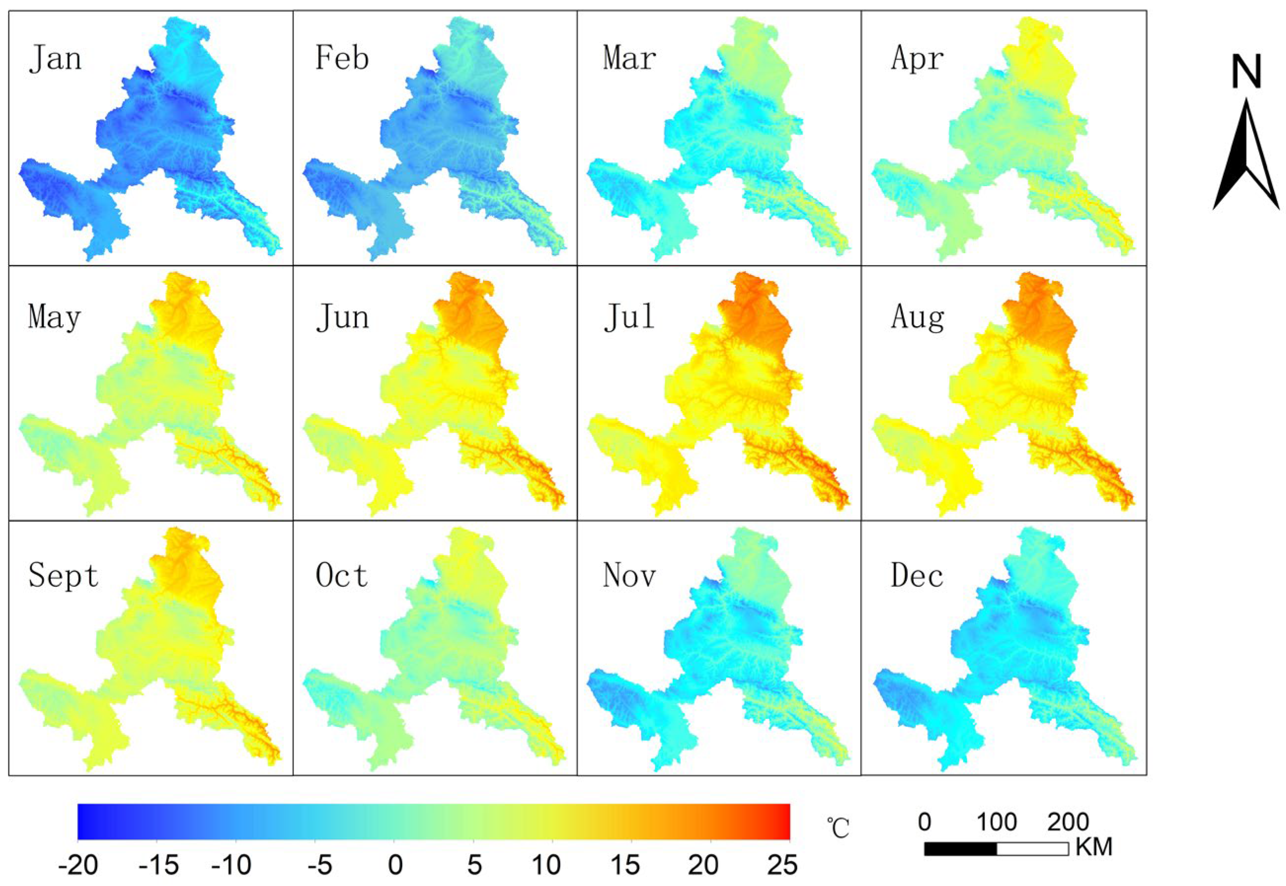
The refined meteorological data (Figure 3) obtained from the multiple regression model and the residal analysis show that the high values of monthly average temperature are mainly found in the southeastern part of the study area (Diebu County and Zhouqu County), and the high temperature in Zhouqu County is mainly found in the area with lower elevation, i.e., the lower right part of the figure. The temperature in Linxia Hui Autonomous Prefecture in the study area is higher than that in Gannan Tibetan Autonomous Prefecture as a whole. From the map, the temperature values in the southwestern part of the study area (Maqu County) show the characteristics of lower temperatures in the west and higher temperatures in the southeast, and the Yellow River source area, Maqu County, is part of the Tibetan Plateau and belongs to the alpine humid climate zone [43]. After merging the DEM data, the simulation reflects the obvious distribution characteristics of temperature elements from the DEM elevation data, and the elevation information is clearly reflected in the resulting display. The spatial distribution characteristics of the monthly average temperature of the seasonally representative months estimated by the distributed climate model in the complex alpine terrain regions are analyzed separately (Figure 4). The temperature of the study area rises gradually from January to July, reaches a maximum value of 24.2 °C in July, and then decreases to a minimum value of −18.1 °C in December. Low temperatures in January, April, July and October mainly occur in high-altitude areas, such as northwest of Maqu County, northeast of Hezuo City, Luqu County, Xiahe County and the junction of Zhuoni County and Diebu County. The high-temperature areas are mainly in low-altitude areas, such as Linxia Prefecture and parts of Diebu County and Zhouqu County. The topography of the study area significantly controls the temperature, and the distribution of temperature with altitude is obvious.

4.3. Cumulative Monthly Average Precipitation and Cumulative Annual Total Precipitation

The precipitation in the study area gradually rose from January to a maximum of 161.93 mm in July (Figure 5), then began to decline and fell to a minimum of 0.35 mm in December. The precipitation in Linxia Hui Autonomous Prefecture was lower than that in Gannan Tibetan Autonomous Prefecture and more clearly differentiated from Gannan Prefecture. The study area shows the characteristics of single-peaked autumn rainfall in western China, with autumn precipitation almost as high as summer and higher than spring. The areas with high precipitation are located at higher altitudes (Figure 6), such as the northwestern part of Maqu County, northeastern part of Hezuo City, Luqu County, Xiahe County and the junction of Zhuoni County and Diebu County, while the areas with low precipitation are mainly located in Linxia Prefecture and some areas of Diebe County in Zhouqu County.

4.4. Error Analysis

From the temperature, we find that the mean error is higher in the spring and summer seasons than in the autumn and winter seasons (

Table 3. Error values of the temperature and precipitation simulation results.

Month	Temperatures ME (°C)	Temperatures RMSE (°C)	Precipitation ME (mm)	Precipitation RMSE (mm)
January	0.585	2.012	−0.061	0.722
February	0.612	2.000	−0.153	1.705
March	0.614	1.941	1.243	4.439
April	0.694	2.210	−1.589	6.993
May	0.843	2.226	−1.842	10.443
June	0.891	2.173	−0.627	12.421
July	0.843	2.133	−5.808	11.523
August	0.758	2.062	−1.916	7.934
September	0.661	1.943	−2.163	8.992
October	0.653	1.925	−0.741	9.731
November	0.683	1.951	0.159	1.129
December	0.635	1.878	−0.104	0.505
Annual average	0.686	2.016	−13.629	79.581

), indicating that the simulation in the spring and summer periods is not as good as that in the autumn and winter seasons, but the mean error is below 1.2. The root mean square error is also higher in the spring and summer seasons than in the autumn and winter seasons. This phenomenon indicates that the temperature difference in the study area is more obvious in the spring and summer seasons, which is consistent with the experimental results. Basic linear regression is used in this study, and the results reach more realistic levels.

From the error table of precipitation, it is obvious that the best simulation is in January, with an ME of −0.061, and the worst simulation is in summer. The maximum precipitation in the study area is in July, which is also the month with the largest ME of −5.808 in this simulation. The precipitation distribution in the study area varies greatly in summer, and the extreme difference is approximately 100 mm. Because of the limited precipitation, the study in this paper focuses on cumulative annual average precipitation, and the RMSE and ME are influenced by the magnitude of the data values themselves [44], so the annual average precipitation land values are larger.

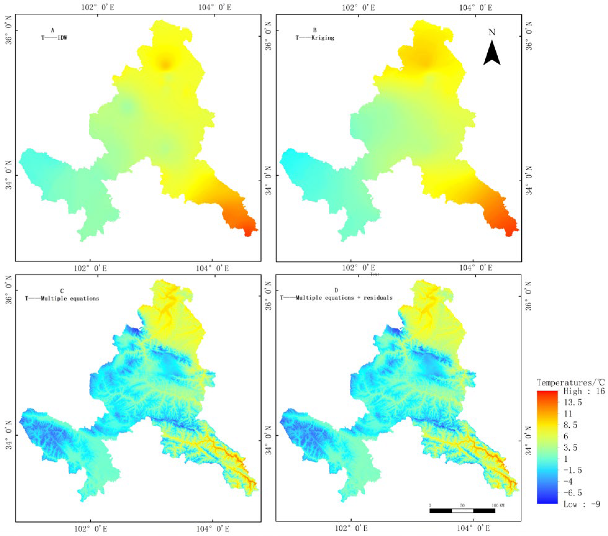
4.5. Comparison of Topographic Spatial Statistics Methods with Common Interpolation Methods

The ordinary kriging interpolation method, IDW interpolation method and “multiple regression + residual analysis” topographic spatial statistics method all have their advantages (Figure 7 and Figure 8). From the ordinary kriging interpolation and IDW interpolation, it can be clearly found that the annual average temperature of the study area increases from southwest to northeast, and the highest value of temperature is found in the southeastern area, i.e., Zhouqu County, and the boundary line is not obvious. In addition, the interpolation method of IDW is applied to the temperature simulation with a more obvious “bull’s eye” phenomenon [45], which is caused by the bias of IDW in the interpolation process with only distance as the weight. From the precipitation results of general kriging interpolation and the IDW interpolated precipitation results, we can notice that the precipitation in the southwestern part of the study area is significantly higher than that in the northern part, showing a decreasing trend before increasing from the southeast to the northwest, when the boundary is less obvious, and the bull’s-eye phenomenon also appears in the IDW interpolation. When only the multivariate model of temperature and precipitation is simulated, the error caused by the data without further correction is larger than that of the topographic spatial statistics method of “multiple regression + residual analysis”. In contrast, the topographic spatial statistics method reflects the horizontal zone pattern of decreasing temperature with increasing latitude and the topographic characteristics of decreasing temperature with increasing altitude. The raster map obtained by the topographic spatial statistics method also reflects the influence of topography on annual precipitation.

The topographic spatial statistics method can not only reflect the horizontal zonal distribution of temperature and precipitation in the study area but also clearly show the changes in temperature and precipitation with increasing altitude. However, general kriging and IDW interpolation do not take into account the influence of topography on meteorological data. The topographic spatial statistics method is more accurate and detailed for temperature and precipitation, taking into account longitude, latitude and altitude, so the topographic spatial statistics method is better than the other two methods.

4.6. Comparison of Precipitation Distributed Model Dataset and Precipitation Product Dataset

By comparing the ME and RMSE with the Chinese 1 km monthly precipitation dataset, it is found that the accuracy of the precipitation dataset obtained in this study is significantly higher than that of the Chinese 1 km monthly precipitation dataset for the study area from 1981 to 2010 (

Table 4. Error values of the precipitation distributed model simulation results compared to the precipitation product dataset.

Month	Precipitation Distributed Model Dataset ME (mm)	Precipitation Distributed Model Dataset RMSE (mm)	Precipitation Product Dataset ME (mm)	Precipitation Product Dataset RMSE (mm)
January	−0.061	0.722	0.41	1.24
February	−0.153	1.705	1.40	2.57
March	1.243	4.439	1.53	5.57
April	−1.589	6.993	0.80	7.57
May	−1.842	10.443	−5.63	17.67
June	−0.627	12.421	3.82	12.13
July	−5.808	11.523	1.49	20.36
August	−1.916	7.934	−6.97	25.28
September	−2.163	8.992	−12.95	25.14
October	−0.741	9.731	−3.86	12.63
November	0.159	1.129	−1.18	5.28
December	−0.104	0.505	1.81	1.84
Annual average	−13.629	79.581	305.83	338.35

). In April and July, the accuracy of the precipitation dataset obtained in this study is slightly lower than that of the Chinese 1 km monthly precipitation dataset, and in the rest of the months, the precipitation distribution model dataset in this study is higher than that of the Chinese 1 km monthly precipitation product dataset.

5. Conclusions

This study is based on the cumulative monthly average temperature and cumulative monthly average precipitation from 1981 to 2010 at 47 stations, as well as geographic coordinates and DEM data of Gannan and Linxia prefectures, and transforms the single-point meteorological station data into the surface-scale level through GIS spatial analysis and multiple regression data analysis to make up for the missing meteorological data. The results of the study were corrected by removing residuals to make the results more accurate. The main conclusions of the study are as follows:

(1) In this study, the GIS spatial analysis and multiple regression data analysis were used to transform the single-point meteorological station data into the surface level to make up for the missing meteorological data, and the residuals were removed to correct the study results, which made the study results more accurate. The model parameters of temperature and precipitation pass the 0.0001 significance test and have a high R. The model simulations of temperature and precipitation are good. The model simulations of both temperature and precipitation are good, which can not only reflect the horizontal distribution pattern of meteorological data but also clearly show the change characteristics of temperature and precipitation with the increase in altitude, i.e., meet the requirements of a fine spatial distribution of climate elements in the study area.

(2) The spatial distribution pattern of temperature is as follows: the temperature in the study area gradually increases from the southwest to the northeast, and Zhouqu County in Linxia and Gannan is the main high-temperature area. The spatial distribution of precipitation is as follows: the precipitation in the southwest of the study area is significantly higher than that in the north, and the precipitation in Linxia is significantly lower than that in Gannan.

(3) The temporal distribution pattern of the temperature distribution model is as follows: the overall temperature at the northeast edge of the Tibetan Plateau is at its lowest level in January, with the highest temperature of only 2.6 °C, and gradually starts to decline after the highest temperature rises to 24.2 °C in July. The spatial distribution of precipitation is as follows: the precipitation in the study area gradually rises from January, to July, when it is its highest, and then starts to decline, and in December, the temporal distribution characteristics of the precipitation distribution model are similar to those of the temperature model, with obvious water-heat synchronization characteristics.

The traditional Interpolation method only takes Into account the latitude and longitude of the sampling points but not the altitude of the sampling points, while the topographic spatial statistics method improves this defect on this basis. Another advantage of the topographic spatial statistics method is the parameter setting of the regression equation; different regression equations are obtained for different study areas, which further improves the accuracy of interpolation on the basis of the original one. The higher the correlation coefficient between meteorological data and latitude and longitude, the better the simulation effect of the topographic spatial statistics method, which indicates the general applicability of the method [6].

In this paper, a new idea to solve the topic of climate analysis in alpine complex terrain regions is proposed through the northeastern margin of the Tibetan Plateau, a region with typical characteristics. In this part of the study, GIS provides important technical support and the powerful spatial computing capability of GIS challenges the existing regional climate analysis of complex terrain to reach further development. This paper introduces topographic factors into the study of temperature and precipitation in alpine complex terrain regions, and the temperature and precipitation model adopted for alpine complex terrain regions is a basic linear regression model simulation. The subsequent research can further enrich the parameters of the model and the model form to get a more accurate and reasonably distributed model of temperature and precipitation in alpine complex terrain regions, according to the research idea of this paper.

References

- Yue, W.Z.; Xu, J.H.; Xu, L.H. A Study on Spatial Interpolation Methods for Climate Variables Based on Geostatistics. Plateau Meteorol. 2005, 24, 974–980. [Google Scholar]
- Tian, H.W.; Li, S.Y. Refined Zonation of Integrated Drought Risk About Summer Maize in He’nan Province. J. Arid. Meteorol. 2016, 34, 852–859. [Google Scholar]
- Song, L.Q.; Tian, Y.; Wu, L. On Comparison of Spatial Interpolation Methods of Daily Rainfall Data: A Case Study of Shenzhen. Geo. Inf. Sci. 2008, 10, 566–572. [Google Scholar]
- Wu, L.; Wu, X.J.; Xiao, C.C. On Temporal and Spatial Error Distributions of Five Precipitation Interpolation Models: A Case of Shenzhen. Geogr. Geo. Inf. Sci. 2010, 26, 19–24. [Google Scholar]
- Liu, Q.; Yan, C.R.; He, W.Q.; Du, J.T.; Yang, J. Dynamic Variation of Accumulated Temperature Data in Recent 40 Years in the Yellow River Basin. J. Nat. Resour. 2009, 24, 147–153. [Google Scholar]
- Guo, J.; Liu, X.N.; Ren, Z.C. An improved method for spatial interpolation of meteorological data based on GIS modules—A case study in Gansu Province. Grassl. Turf 2011, 31, 41–45. [Google Scholar]
- Price, D.T.; McKenney, D.W.; Nalder, I.A.; Hutchinson, M.F.; Kesteven, J.L. A comparison of two statistical methods for spatial interpolation of Canadian monthly mean climate data. Agric. For. Meteorol. 2000, 101, 81–94. [Google Scholar] [CrossRef]
- Chen, F.; Dong, M.Y.; Ji, C.X. Application of A Comprehensive Analysis Method on Hourly Surface Air Temperature Interpolation over A Complex Terrain Region. Plateau Meteorol. 2016, 35, 1376–1388. [Google Scholar]
- Liu, Y.J.; Zhao, X.M.; Gan, D.Q. Kriging Interpolation Analysis of Orebody Based on Borehole Data. China Tungsten Ind. 2021, 36, 31–37. [Google Scholar]
- Li, X.; Cheng, G.D.; Lu, L. Comparison of Spatial Interpolation Methods. Adv. Earth Sci. 2000, 15, 260–265. [Google Scholar]
- Gao, T.P.; Xue, W.; He, Y.Q.; Li, C.M. Discussion on the Relationship between Ecological Security and Economic Development in the Upper Reaches of the Yellow River in study area. Ecol. Econ. 2021, 37, 1–15. [Google Scholar]
- Li, H.M.; Ma, Y.S. Application on classification of Qinghai grassland by advanced comprehensive and sequential classification. Acta Prataculturae Sin. 2009, 18, 76–82. [Google Scholar]
- Zhang, Y.Q.; Liu, Q.; Yan, C.R.; He, W.Q.; Liu, S. Methodology for rasterizing accumulated temperature data in the Yellow River Basion. Acta Ecol. Sin. 2009, 29, 5580–5585. [Google Scholar]
- Lin, Z.H.; Mo, X.G.; Li, H.X. Comparison of Three Spatial Interpolation Methods for Climate Variables in China. Acta Geogr. Sin. 2002, 57, 47–56. [Google Scholar]
- Feng, Z.M.; Yang, Y.Z.; Ding, X.Q.; Lin, Z.H. Optimization of the spatial interpolation methods for climate resources. Geogr. Res. 2004, 23, 357–364. [Google Scholar]
- Zhang, H.L.; Ni, S.X.; Deng, Z.W. A Method of Spatial Simulating of Temperature Based Digital Elevation Model(DEM) in Mountain Area. J. Mt. Res. 2002, 20, 360–364. [Google Scholar]
- Pan, Y.Z. Smart Distance Searching-based and DEM-informed Interpolation of Surface Air Temperature in China. Acta Geogr. Sin. 2004, 59, 366–374. [Google Scholar]
- Zhen, J.G.; Chen, Q.G.; Han, T. Catchment precipitation estimation with GIS modules and its improvements in Gansu Province. Sci. Meteorol. Sin. 2009, 29, 4467–4474. [Google Scholar]
- Song, J.R.; Hu, Y.; Tong, Z.C.; Liu, M.; Gao, J.; Zhang, Y.; Man, W. A comparative study on spatial interpolation methods of precipitation in Xinjiang. Agric. Sci. J. Yanbian Univ. 2021, 43, 41–46. [Google Scholar]
- Li, T. Comparative Analysis of IDW and PER Spatial Interpolation of Rainfall Data in Liaoning Province. Shaanxi Water Resour. 2021, 10, 21–23. [Google Scholar]
- Luo, L.; Dai, C.L.; Li, M.L.; Wu, Y. Analysis and comparison of Spatial interpolation of Multi-year average precipitation in Heilongjiang Province based on GIS. Jilin Water Resour. 2021, 10, 9–16. [Google Scholar]
- Bi, B.G.; Xu, J.; Lin, J. Method of Area Rainfall Calculation and Its Application to Haihe Valley. Meteorol. Mon. 2003, 29, 39–42. [Google Scholar]
- Liang, S.X.; Liu, X.H.; Cheng, X.W.; Yang, Y.Q.; Xu, M. Distance-Weighted Average Method to Calculate the Average Surface Rainfall in the Watershed. Innovation of Meteorological Science and Technology and Development of Atmospheric Science in the New Century. In Proceedings of the 2003 Annual Meeting of the Chinese Meteorological Society on “Hydro-meteorological Aspects of the Huai River Flood of 03.7”, 2003-12. Available online: http://www.progressingeography.com/EN/10.11820/dlkxjz.2014.07.003 (accessed on 25 September 2021).
- Juan, L.L.; Wang, J.; Li, H.B. Analysis of the spatial variability of rainfall in Wuding River Basin. Geogr. Res. 2002, 21, 434–440. [Google Scholar]
- Xu, B.R. Hydrologic Cycle Characteristics of Land-Atmosphere System in Heihe River Basin Based on GIS and RIEMS. Doctoral Dissertation, Lanzhou University, Lanzhou, China, 2015. [Google Scholar]
- Ashraf, M.; Loftis, J.C.; Hubbard, K.G. Application of geostatistics to evaluate partial weather station networks. Agric. For. Meteorol. 1997, 84, 255–271. [Google Scholar] [CrossRef]
- Lu, G.Y.; Wong, D.W. An adaptive inverse-distance weighting spatial interpolation technique. Comput. Geosci. 2008, 34, 1044–1055. [Google Scholar] [CrossRef]
- Nalder, I.A.; Wein, R.W. Spatial interpolation of climatic Normals: Test of a new method in the Canadian boreal forest–ScienceDirect. Agric. For. Meteorol. 1998, 92, 211–225. [Google Scholar] [CrossRef]
- Goovaerts, P. Geostatistical approaches for incorporating elevation into the spatial interpolation of rainfall. J. Hydrol. 2000, 228, 113–129. [Google Scholar] [CrossRef]
- Wang, Z.G.; Wang, X.L.; Ji, Z.J.; Wang, S.P.; Fu, W.R. Spatial and Temporal Variation Characteristics of Different Intensity Precipitation in Flood Season over the study area during 1976–2019. Desert Oasis Meteorol. 2022, 16, 56–63. [Google Scholar]
- Zou, S.B.; Qian, J.K.; Xu, B.R.; Tu, Z.Y.; Zhang, W.Y.; Ma, X.L.; Liang, Y. Spatiotemporal changes of ecosystem health and their driving mechanisms in alpine regions on the northeastern Tibetan Plateau. Ecol. Indic. 2022, 143, 109396. [Google Scholar] [CrossRef]
- Wang, W.J.; Zhao, X.Y.; Wan, W.Y.; Li, H.; Xue, B. Variation of vegetation coverage and its response to climate change in study area from 2000 to 2014. Chin. J. Ecol. 2016, 35, 2494–2504. [Google Scholar]
- Yao, T.D. TPE international program: A program for coping with major future environmental challenges of the Third Pole region. Prog. Geogr. 2014, 7, 23–31. [Google Scholar]
- Zhao, X.Y.; Li, W. College of Geography and Environment Science, Northwest Normal University. Review of Gannan research in Chinese geography. Geogr. Res. 2019, 38, 743–759. [Google Scholar]
- Wu, G.H. The Natural Conditions and Ecological Protection of Study Area; Gansu People’s Publishing House: Lanzhou, China, 2010. [Google Scholar]
- Hu, K.; Huang, G.; Huang, R. The Impact of Tropical Indian Ocean Variability on Summer Surface Air Temperature in China. J. Clim. 2011, 24, 5365–5377. [Google Scholar] [CrossRef]
- Xiao, L.; Li, D.-L.; Wang, H. New Evolution Features of Autumn Rainfall in West China and Its Responses to Atmospheric Circulation. Plateau Meteorol. 2013, 32, 1019–1031. [Google Scholar]
- Lin, S.; Zhao, J.H.; Wen, Q.U. Abnormal Circulation that Affects Precipitation over Northwest China in Summer and Autumn in 2003. J. Catastrophology 2004, 19, 62–67. [Google Scholar]
- Jia, X. Causality Analysis of Autumn Rainfall Anomalies in China in 2007. Meteorol. Mon. 2008, 34, 86–94. [Google Scholar]
- Wang, H.J.; Wang, Z.C.; Wang, K.; Peng, C.; Zhu, Y.G. Anomalous Circulation Characteristics of Autumn Rain and Its Cause over West China in 2017. J. Arid. Meteorol. 2018, 36, 743–750. [Google Scholar]
- Wang, Y.L. Protection and reconstruction of ecologically fragile areas on the Qinghai-Tibet Plateau in the context of main function zoning. J. Southwest Univ. Natl. (Humanit. Soc. Sci.) 2008, 4, 42–46. [Google Scholar]
- Liu, Y.; Zou, S.B. A study on the distributing climatic models in arid mountainous area—Distributing temperature and precipitation models in high spatial resolution in the Qilian Mountains. J. Lanzhou Univ. 2006, 42, 7–12. [Google Scholar]
- Chai, C.W.; Xu, X.Y.; Zhang, L. Analysis on climatic characteristics in Maqu County. Grassl. Turf 2012, 32, 74–77. [Google Scholar]
- Chu, T.W.; Shirmohammadi, A. Evaluation of the SWAT model’s hydrology component in the Piedmont physiographic region of Maryland. Trans. Asae 2004, 47, 1057–1073. [Google Scholar] [CrossRef]
- Xi, J.Y.; Guo, Y.; Shan, Z.X. Comparative study of GIS-based spatial interpolation methods for soil organic matter content. Heilongjiang Sci. Technol. Inf. 2012, 35, 80–81. [Google Scholar]