Research on Radar Echo Extrapolation Method by Fusing Environment Grid Point Field Information

Abstract

Short-term extrapolation by weather radar observations is one of the main tools for making weather forecasts. Recently, deep learning has been gradually applied to radar extrapolation techniques, achieving significant results. However, for radar echo images containing strong convective systems, it is difficult to obtain high-quality results with long-term extrapolation. Additionally, there are few attempts and discussions to incorporate environmental factors governing the occurrence and development of convective storms into the training process. To demonstrate the positive effect of environmental factors on radar echo extrapolation tasks, this paper designs a three-dimensional convolutional neural network. The paper outlines the processing steps for matching radar echo images with environmental data in the spatio–temporal dimension. Additionally, it develops an experimental study on the effectiveness of seven physical elements and their combinations in improving the quality of radar echo extrapolation. Furthermore, a loss function is adopted to guide the training process of the model to pay more attention to strong convective systems. The quantitative statistical evaluation shows the critical success index (CSI) of our model’s prediction is improved by 3.42% (threshold = 40 dBZ) and 2.35% (threshold = 30 dBZ) after incorporating specific environmental field data. Two representative cases indicate that environmental factors provide essential information about convective systems, especially in predicting the birth, extinction, merging, and splitting of convective cells.

1. Introduction

Nowcasting refers to the weather forecast for the next 0–6 h (especially for 0–2 h) kilometer and minute level, which is a social service to prevent sudden catastrophic weather in the area [1]. Its forecast objects mainly include thunderstorms, heavy precipitation, snowstorms, and other strong convective weather with rapid development, complex changes, and strong destructive power. How to accurately predict future weather changes by nowcasting is an important research topic to mitigate or even prevent strong convective disasters.

The weather forecasting methods are mainly divided into two categories: numerical weather forecasting (NWP) and extrapolation methods based on observation data from radar or satellite. NWP is a method based on solving a series of partial differential equations governing atmospheric motion [2]. It quantitatively describes the physical state of the atmosphere. However, the mass computation makes it difficult to finish fast real-time forecasts by NWP. Additionally, it is hard to assimilate observations at the convective scale, which makes it difficult to describe sub-grid-scale physical processes. Small perturbations in the initial boundary conditions can seriously affect the final forecast accuracy [3]. These characteristics determine that NWP is suitable for long-term large-scale forecasts but not for short-term small- and medium-scale forecasts.

Since the radar echo data has high spatio–temporal resolution and intuitional information, extrapolation based on real-time weather radar data become the mainstream method for nowcasting [4]. Radar extrapolation technology refers to predicting radar echo images in the future based on the sequence of radar echo images in the past. High-quality radar extrapolation results are the basis for a variety of subsequent weather system identification and forecasting algorithms. The traditional radar extrapolation methods mainly include the storm cell identification and tracking algorithm (SCIT); the thunderstorm identification, tracking, analysis, and nowcasting (TITAN); tracking radar echoes with the correlation algorithm (TREC); and the optical flow method. The SCIT and TITAN algorithms focus on the identification and tracking of storm cells. They calculate the motion vectors of the cell by determining and tracking the position of the cell’s centroid [5,6]. However, they selectively ignore weak echo information in the forecasting process because it only focuses on the motion trajectory of a single storm cell. Tracking radar echoes with a correlation algorithm (TREC) calculates the optimal correlation between pairs of local regions. By comparing the echo images of adjacent moments, TREC obtains the motion vector of each region in the echo image. This motion vector then predicts the echo position in the future. The methodology described in [7] is based on this approach. It will generate many disordered motion vectors when tracking echoes generate and change very fast, leading to poor performance. The optical flow method is used to obtain the optical flow field by pixel-level matching to obtain the motion vector of each pixel in the image, and then extrapolate the forecast of the echo image based on this optical flow field [8,9,10]. The optical flow method is based on change rather than motion trajectory tracking based on invariant features. It can only predict the movement of storm cells by optical flow motion, not the change in storm cell size and intensity. Therefore, the performance decreases drastically with the increase in lead time [11].

In recent years, many deep learning models have been proposed to improve forecasting performance. Neural networks can learn and model complex weather motion patterns from large historical data sets with their powerful feature extraction and nonlinear mapping capabilities. A series of neural networks for radar echo prediction have emerged [12,13,14,15,16,17,18,19,20,21,22]. The first end-to-end extrapolation model for nowcasting was proposed by Shi et al. [12]. They improved the traditional long short-term memory (LSTM) unit by replacing fully connected layers with convolutional layers. This modification proposes the ConvLSTM network, in which the extraction of spatial features is implemented with convolutional layers and the LSTM unit is responsible for capturing the correlation between echoes at different moments. The extrapolation performance is significantly improved compared to the conventional optical flow method. Furthermore, Shi et al. [13] also proposed the TrajGRU network to further capture scaling and rotating objects. Additionally, Wang et al. [14,15,16] proposed a series of recurrent neural network (RNN) structures to refine the traditional ConvLSTM. In addition to RNN, Agrawal et al. [17] treated radar echo extrapolation as an image-to-image conversion problem, using the data-driven approach without considering the actual physical mechanism, and used U-Net for direct prediction. Kim et al. [18] used 3D convolution to extract the spatio–temporal information of the video sequence frames. Different from the end-to-end models above, in order to generate two prediction probability vectors to predict future radar echoes, Klein et al. [19] proposed adding a dynamic convolutional layer to the traditional convolutional neural network. However, the above approach using the traditional mean square error loss leads to blurred image output from the model. Therefore, Wang et al. [20] employed conditional generative adversarial networks (CGAN) and 3D convolutional networks to improve the extrapolation performance.

Despite their better performance, however, literature [4] points out that most of the deep learning methods proposed at present only use historically recorded radar echo sequences as input, omitting the fact that the development of convection is highly related to the information rooting in the atmospheric environment. The dynamical structure of the storm and its potential development depend heavily on three physical elements: the thermal instability of the environment, the vertical wind shear, and the vertical distribution of water vapor [23]. It is apparently true that radar echoes do not contain the above physical information, which can lead to different evolving processes of echoes even for similarly observed input echoes [24,25]. In other words, similar echo sequence inputs may have different directions under different environmental field constraints. In particular, it is difficult to predict generation, extinction, splitting, merging, and other phenomena only based on radar echoes. Some experiments have been made to integrate the radar data into the NWP [26,27] or use some extra data to improve the extrapolation, such as dual-polarization radar data [28] and the high-resolution rapid refresh model (HRRR) [29]. However, so far, no attempt has been made to incorporate environmental field information into the extrapolation process.

In order to provide intuitive and effective macroscopic physical constraints on the extrapolation process and improve the performance of the extrapolation, this paper proposes the idea of building a radar echo extrapolation model with the participation of real-time environmental field data. The environment field data can give useful information that is consistent with the evolution trend of radar echoes. The combination of radar data and environmental field data describes both the convective system intensity distribution as well as the external conditions that constrain the evolution of the convective system. Thus, it improves the model’s prediction capability of radar echo evolution comprehensively and allows for a more reasonable interpretation of the prediction results from a meteorological perspective. The design idea for the extrapolation model is to build a multi-channel 3D convolutional network consisting of three functional modules: encoding, inference, and decoding. There are two kinds of encoders: the echo encoder and the environment field encoder. The feature layers from the two types of encoders are stacked and sent to the inferer for fusion, which is then processed by the decoder to obtain the extrapolation result corrected by the environment field.

The paper is organized as follows: Section 2 describes the proposed method and the data used in this experiment; Section 3 and Section 4 show the test results and the analysis of different cases. Section 5 concludes with a discussion.

2. Materials and Methods

2.1. Data

2.1.1. Radar Echo Data and Samples

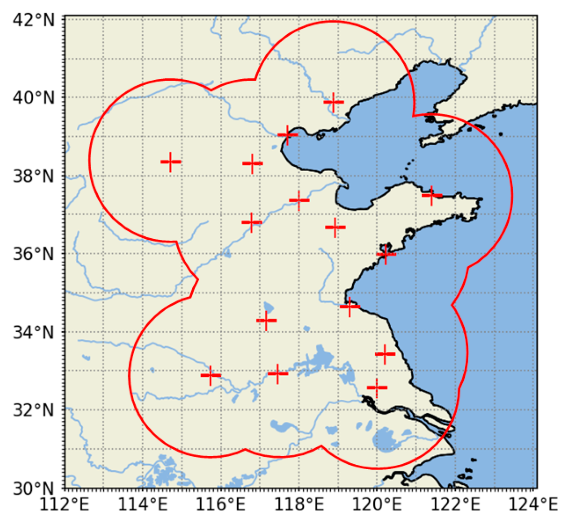
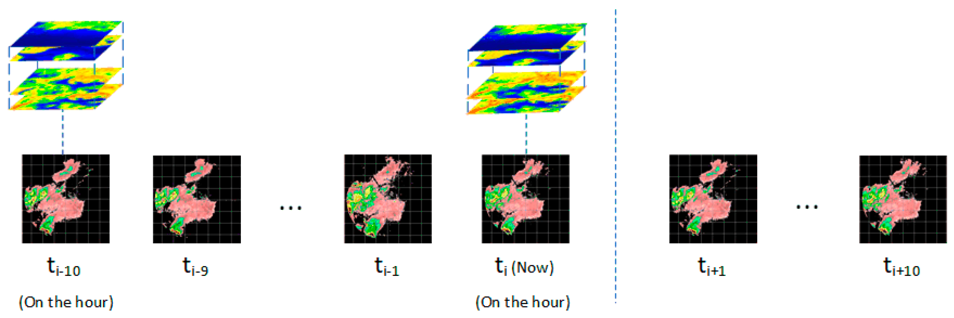
The radar echo data are obtained from S-band Doppler weather radar data provided by the China Meteorological Administration, involving 15 radar sites at different locations in North and East China [30,31]. The stations’ locations and scanning ranges are shown in Figure 1. The scan period is from May 2015 to October 2016. The radar completes a scan every 6 min on average, and the scan radius is up to 230 km. Each scan includes nine elevation angles from 0.5° to 19.5°. Based on the above data, the composite reflectivity image is obtained according to the following steps: Firstly, the radar base data is converted from polar coordinate format to Cartesian coordinate format by bilinear interpolation in the horizontal dimension. Then, it is interpolated in the vertical direction to obtain three-dimensional equidistant grid point field data with a horizontal resolution of 2 km × 2 km and a vertical resolution of 0.5 km. The height ranges from 0.5 km to 7.5 km. Finally, select the maximum value in all height layers to generate a 256 × 256 radar composite reflectivity image. As shown in Figure 2, every successive 21 radar composite reflectivity images are considered a sample, and each image’s size is 256 × 256, where the 11th image must be scanned within 3 min before and after the hour. The first 11 images in the sample are used as model inputs, and the last 10 images are used as real labels. A total of 9539 samples are collected under the condition that the sample contains strong echoes continuously. The samples are randomly divided into a training set: validation set: test set = 4:1:1, with the numbers of training, validation, and test samples being 6360, 1590, and 1589, respectively.

2.1.2. Environment Grid Point Data

The environment field data is extracted from the fifth generation of Global Atmospheric Reanalysis (ERA5) data from the European Centre for Medium-Range Weather Forecasts. ERA5 provides hourly real-time estimates of atmospheric, terrestrial, and oceanic climate variables. The data cover the Earth on a 30 km grid and use 137 altitudes from the surface to an altitude of 80 km to parse the atmosphere. ERA5 combines model data with observational data from around the world to form a globally complete and consistent data set [32]. We chose seven types of environmental field data covering China from May 2015 to October 2016, including temperature, relative humidity, specific humidity, divergence, geopotential height, vertical velocity, and relative vorticity [33]. These physical quantities are considered to be important factors affecting atmospheric movement and precipitation. Each environment field contains seven height levels: 100 hPa, 200 hPa, 300 hPa, 500 hPa, 700 hPa, 850 hPa, and 925 hPa. Heights are considered channels. Every radar echo sample includes two frames of environmental field data: the first echo scan time and the 11th echo scan time. The extraction range is a rectangular area of 1024 km × 1024 km centered on the radar base station. Since the original environmental field data is a 0.25° × 0.25° equal latitude and longitude grid field, it needs to be transformed into an equal distance grid field by bilinear interpolation. After the completion of interpolation, the spatial resolution of the isometric grid field is 32 km × 32 km, and the size of the grid field is 32 × 32.

2.2. Model

2.2.1. Three-Dimensional Convolution

In recent years, a convolutional neural network (CNN) has been considered one of the core algorithms in the field of image processing. It can fully learn the features of an image using a small number of parameters while preserving the spatial structure of the image. However, traditional 2D convolution has some limitations in processing video data. Assuming the size of a video is T × H × W (T is the number of frames of the video, H is the height of a frame, and W is the width of a frame), the 2D convolution kernel will perform the convolution operation in the dimension of H × W and output a single image. Hence, it will completely lose temporal information, as shown in Figure 3a.

Du et al. [34] proposed 3D convolution to deal with problems such as video classification or prediction. Compared with 2D convolution, 3D convolution expands the temporal dimension, as shown in Figure 3b, which enables the convolutional kernel to extract features in both the temporal and spatial dimensions at the same time. Therefore, we chose 3D convolution as the basic unit of our neural network.

2.2.2. Network Structure

We use a late fusion strategy to fuse the echo sequence and environmental information [35]. The neural network consists of four main components: the radar echo encoder, the environment field encoder, inference, and decoder. The network structure is shown in Figure 4. Detailed parameters are shown in Appendix A,

Table A1. The parameters of encoders.

Module	Layer	Kernal Size/Padding/Stride	In/Out Channels	Output Size
Radar Echo Encoder	Conv1-1	4 × 3 × 3/1/1	1/32	10 × 256 × 256
	Conv1-2	3 × 3 × 3/1/1	32/32	10 × 256 × 256
	Pooling-1	-	32/32	10 × 128 × 128
	Conv2-1	3 × 3 × 3/1/1	32/64	10 × 128 × 128
	Conv2-2	3 × 3 × 3/1/1	64/64	10 × 128 × 128
	Pooling-2	-	64/64	10 × 64 × 64
	Conv3-1	3 × 3 × 3/1/1	64/128	10 × 64 × 64
	Conv3-2	3 × 3 × 3/1/1	128/128	10 × 64 × 64
	Pooling-3	-	128/128	10 × 32 × 32
	Conv4-1	3 × 3 × 3/1/1	128/256	10 × 32 × 32
	Conv4-2	3 × 3 × 3/1/1	256/256	10 × 32 × 32
	Pooling-4	-	256/256	5 × 16 × 16
Environment Encoder	Upsample	-	7/7	5 × 32 × 32
	Conv1	3 × 3 × 3/1/1	7/32	5 × 32 × 32
	Conv2	3 × 3 × 3/1/1	32/32	5 × 32 × 32
	Conv3	3 × 3 × 3/1/1	32/64	5 × 32 × 32
	Conv4	1 × 17 × 17/0/1	64/64	5 × 16 × 16
	Conv5	3 × 3 × 3/1/1	64/128	5 × 16 × 16
	Conv6	3 × 3 × 3/1/1	128/128	5 × 16 × 16

and

Table A2. The parameters of inference and decoder.

Layer	Kernal Size/Padding/Stride	In/Out Channels	Output Size
Inference-1	3 × 3 × 3/1/1	(256 + 128 × Env Input Num)/256	5 × 16 × 16
Inference-2 × 4	3 × 3 × 3/1/1	256/256	5 × 16 × 16
Upsample-1	-	256/256	10 × 32 × 32
Conv1-1	3 × 3 × 3/1/1	256/128	10 × 32 × 32
Conv1-2	3 × 3 × 3/1/1	128/128	10 × 32 × 32
Upsample-2	-	128/128	10 × 64 × 64
Conv2-1	3 × 3 × 3/1/1	128/64	10 × 64 × 64
Conv2-2	3 × 3 × 3/1/1	64/64	10 × 64 × 64
Upsample-3	-	64/64	10 × 128 × 128
Conv3-1	3 × 3 × 3/1/1	64/32	10 × 128 × 128
Conv3-2	3 × 3 × 3/1/1	32/32	10 × 128 × 128
Upsample-4	-	32/32	10 × 256 × 256
Conv4-1	3 × 3 × 3/1/1	32/32	10 × 256 × 256
Conv4-2	3 × 3 × 3/1/1	32/1	10 × 256 × 256

.

We summarize the main structure of our proposed model as follows: The radar echo images and the environment fields are each sent to an exclusive encoder to obtain feature maps. The maps are stacked in the channel dimension and fed into the inference and decoder to obtain the final output.

The radar echo encoder is responsible for capturing the spatio–temporal information in the radar echo sequence, which can encode the high-dimensional raw data into the low-dimensional feature space. The encoder consists of four encoding blocks, each of which contains two convolutional blocks and an average pooling operation. The convolution block first performs a 3D convolution, followed by a batch normalization [36], and finally, the model nonlinear representation is enhanced by a Leaky Relu activation function [37] output with a slope of 0.2. The number of feature channels is doubled, and the spatial dimensional resolution is halved for each encoding block passed. The average pooling layer of the last encoding blocks takes on the role of halving the temporal resolution.

The environmental field encoder is similar to the radar echo encoder. However, the temporal resolution of the environmental field is lower than that of the radar echo sequence. Therefore, we first perform linear interpolation in the temporal dimension of the environmental field in order to align the outputs of the two encoders in the temporal dimension. Secondly, as the environment field represents a wider spatial range than the radar, this paper uses a large convolution kernel instead of pooling for spatial dimensionality reduction in order to fuse the environment information outside the radar detection region.

The encoders extract various feature maps from the radar echo sequence and the environment fields. These feature maps with the same spatio–temporal dimension are stacked in the channel dimension and entered into the inference. The role of the inference is to learn the correlation between the radar echoes and the environmental fields and to efficiently fuse the features of both. It consists of a series of convolutional blocks. The number of channels in the fused feature map remains constant in this module.

The decoder aims to transform the feature map provided by the inference into an output with the same resolution as the input echo sequence. Its structure is similar to that of the radar echo encoder, but the average pooling layers are replaced with upsampling layers in the decoder blocks, and the number of feature map channels is halved for each decoder block, where the first decoder block also takes on the role of restoring the temporal resolution. The multi-layer output of the decoder finally turns into a single-channel image sequence by a 1 × 1 convolution operation, which is the output of the model.

2.3. Loss Function

The presence of high-reflectivity regions is often accompanied by strong convective weather. However, the number of high-reflectivity grid points only accounts for a very small fraction of the total grid points in the whole training set. The information provided by the high-reflectivity regions is ignored during the training stage due to their small share, so it is difficult for the model to predict the appearance of strong convective areas. Therefore, we decide to train the model with a weighted mean square error (WMSE) loss function. This loss function assigns a higher weight to the high-reflectivity region to make the model pay more attention to the accuracy of the high-reflectivity region [13].

$$\mathrm{WMSE}={\sum }_{h=1}^{10}{\sum }_{x=1}^{256}{\sum }_{y=1}^{256}{\mathrm{W}\mathrm{e}\mathrm{i}\mathrm{g}\mathrm{h}\mathrm{t}\mathrm{s}}_{(h,x,y)}\times {({I^{\prime }}_{(h,x,y)}-I_{(h,x,y)})}^2$$

(1)

$$\mathrm{Weights}=\left\{\begin{array}{cc}1,\hfill & I_{(h,x,y)}\in (-\infty , 30 \mathrm{dBZ}]\hfill \\ 2,\hfill & I_{(h,x,y)}\in (30 \mathrm{dBZ}, 35 \mathrm{dBZ}]\hfill \\ 3,\hfill & I_{(h,x,y)}\in (35 \mathrm{dBZ}, 40 \mathrm{dBZ}]\hfill \\ 5,\hfill & I_{(h,x,y)}\in (40 \mathrm{dBZ}, 45 \mathrm{dBZ}]\hfill \\ 10,\hfill & I_{(h,x,y)}\in (45 \mathrm{dBZ}, +\infty )\hfill \end{array}\right.$$

(2)

In Equations (1) and (2), I_(h,x,y) represents the reflectivity at the position _(h,x,y) in the observed image sequence. I′_(h,x,y) represents the reflectivity at the position _(h,x,y) in the predicted image and Weights_(h,x,y) is the weight value corresponding to that point. The weight values are set based on the reflective value distribution of different thresholds in the training data.

3. Results

3.1. Training Parameters

The model’s parameters are optimized by the Adam optimizer with a learning rate of 0.001 and decay coefficient betas of (0.9, 0.999). The batch size is set to 8. We trained the model for 50 epochs, and all the model’s loss curves have converged. The epoch with the lowest WMSE on the validation set is selected for testing.

3.2. Pixel-Level Test

3.2.1. Pixel-Level Evaluation Indicators

We use the skill scores of forecasts to test the performance of models on the test set. By setting different reflectivity thresholds, the pixel in the echo image above the threshold is recorded as “yes”, and the pixel below the threshold is recorded as “no”. Then count the number of true positives (TP), false positives (FP), false negatives (FN), and true negatives (TN) from the distribution of “yes” or “no” points in the predicted image and the observed image. The confusion matrix for the classification result is shown in

Table 1. Confusion matrix for classification results.

	Observed “Yes”	Observed “No”
Predicted “yes”	TP	FP
Predicted “no”	FN	TN

.

We introduce five forecast evaluation metrics: the probability of detection (POD), false alarm ratio (FAR), critical success index (CSI), equitable threat score (ETS), and Heidke skill score (HSS) [38]. POD indicates how many positive cases are correctly predicted. FAR indicates the ratio of the predicted positive cases that do not occur; CSI represents a comprehensive evaluation of the effect of both “yes” and “no” forecasts [39]; ETS penalizes false or missed reporting and gives a fair evaluation for prediction [40]; HSS shows the improvement of the accuracy of the actual forecast over that of the random forecast. The computational formula for each index is shown below.

$$\mathrm{POD}=\frac{\mathrm{TP}}{\mathrm{TP}+\mathrm{FN}},$$

(3)

$$\mathrm{FAR}=\frac{\mathrm{FP}}{\mathrm{TP}+\mathrm{FP}},$$

(4)

$$\mathrm{CSI}=\frac{\mathrm{TP}}{\mathrm{TP}+\mathrm{FN}+\mathrm{FP}},$$

(5)

$$\mathrm{HSS}=\frac{2\times (\mathrm{TP}\times \mathrm{TN}-\mathrm{FN}\times \mathrm{FP})}{(\mathrm{TP}+\mathrm{FP})\times (\mathrm{FP}+\mathrm{TN})+(\mathrm{TP}+\mathrm{FN})\times (\mathrm{FN}+\mathrm{TN})},$$

(6)

$$\mathrm{ETS}=\frac{\mathrm{TP}-\mathrm{REF}}{\mathrm{TP}-\mathrm{REF}+\mathrm{FP}+\mathrm{FN}},\mathrm{REF}=\frac{(\mathrm{TP}+\mathrm{FN})\times (\mathrm{TP}+\mathrm{FP})}{\mathrm{TP}+\mathrm{TN}+\mathrm{FP}+\mathrm{FN}},$$

(7)

3.2.2. Pixel-Level Test Results

We first examine the performance of extrapolation after adding different types of environmental fields to the model. We divide the seven environmental fields into three categories: (1) divergence, vertical velocity, relative vorticity, and geopotential height as the dynamic field; (2) relative humidity and specific humidity as the humidity field; and (3) temperature as the temperature field. The performance of adding a single environment field or the combination of a category is shown in

Table 2. Test results of 3D-CNN models with different environment fields (threshold = 40 dBZ).

Environment	POD↑	FAR↓	CSI↑	ETS↑	HSS↑
Without Environment	0.3972	0.5157	0.2791	0.2763	0.4330
Divergence	0.4445	0.4851	0.3133	0.3104	0.4738
Vertical Velocity	0.4314	0.5267	0.2915	0.2885	0.4478
Vorticity	0.3402	0.4713	0.2610	0.2586	0.4109
Geopotential Height	0.4254	0.5268	0.2887	0.2858	0.4445
Relative Humidity	0.4725	0.5383	0.3047	0.3015	0.4634
Specific Humidity	0.4240	0.5119	0.2935	0.2906	0.4503
Temperature	0.4037	0.5128	0.2833	0.2805	0.4381
Dynamic	0.3867	0.4822	0.2843	0.2816	0.4395
Humidity	0.4434	0.5300	0.2956	0.2926	0.4527
Dynamic and Humidity	0.4295	0.4966	0.3017	0.2988	0.4601
Dynamic and Temperature	0.3977	0.4701	0.2940	0.2913	0.4512
Humidity and Temperature	0.4255	0.5169	0.2924	0.2895	0.4490
All Environment Fields	0.3754	0.4925	0.2752	0.2725	0.4283

,

Table 3. Test results of 3D-CNN models with different environment fields (threshold = 30 dBZ).

Environment	POD↑	FAR↓	CSI↑	ETS↑	HSS↑
Without Environment	0.7142	0.3238	0.5322	0.5160	0.6807
Divergence	0.7423	0.3114	0.5557	0.5399	0.7012
Vertical Velocity	0.7623	0.3512	0.5396	0.5227	0.6866
Vorticity	0.7232	0.3214	0.5387	0.5226	0.6864
Geopotential Height	0.7671	0.3631	0.5337	0.5164	0.6811
Relative Humidity	0.7597	0.3387	0.5469	0.5304	0.6931
Specific Humidity	0.7537	0.3369	0.5450	0.6915	0.5285
Temperature	0.7462	0.3428	0.5372	0.5205	0.6846
Dynamic	0.6916	0.2963	0.5356	0.5201	0.6843
Humidity	0.7689	0.3532	0.5415	0.5246	0.6882
Dynamic and Humidity	0.7465	0.3316	0.5447	0.5284	0.6914
Dynamic and Temperature	0.7257	0.3108	0.5468	0.5310	0.6936
Humidity and Temperature	0.7560	0.3441	0.5414	0.5247	0.6882
All Environment Fields	0.6921	0.3055	0.5306	0.5148	0.6797

and

Table 4. Test results of 3D-CNN models with different environment fields (threshold = 20 dBZ).

Environment	POD↑	FAR↓	CSI↑	ETS↑	HSS↑
Without Environment	0.8102	0.1655	0.6980	0.6680	0.8009
Divergence	0.8372	0.1675	0.7165	0.6874	0.8147
Vertical Velocity	0.8288	0.1742	0.7055	0.6754	0.8063
Vorticity	0.8349	0.1804	0.7053	0.6750	0.8060
Geopotential Height	0.8442	0.1937	0.7019	0.6709	0.8030
Relative Humidity	0.8285	0.1693	0.7088	0.6792	0.8090
Specific Humidity	0.8311	0.1731	0.7079	0.6781	0.8082
Temperature	0.8383	0.1860	0.7036	0.6729	0.8045
Dynamic	0.7948	0.1494	0.6974	0.6679	0.8009
Humidity	0.8341	0.1790	0.7057	0.6755	0.8063
Dynamic and Humidity	0.8188	0.1689	0.7020	0.6720	0.8038
Dynamic and Temperature	0.8085	0.1566	0.7030	0.6735	0.8049
Humidity and Temperature	0.8406	0.1836	0.7070	0.6766	0.8071
All Environment Fields	0.7990	0.1582	0.6947	0.6647	0.7986

.

Table 2, Table 3 and Table 4 show that: (1) with the increase in the threshold, all indicators show a decreasing trend. Because the area occupied by the higher reflectivity region is smaller and changes more drastically, it is more difficult to predict the location of the high reflectivity region. (2) From an overall perspective, the POD and CSI of the extrapolation model with the introduction of the environment field are generally improved. The FAR in the high-reflectivity region is generally reduced. (3) Some specific environmental information can improve the extrapolation effect to a certain extent. For example, relative humidity reflects the density of water vapor particles in the region, and divergence reflects the aggregation or dispersion movement of the atmosphere. Additionally, the improvement gets more and more obvious as the threshold increases. The addition of the divergence field results in a 2.05% improvement in the HSS scores with a threshold of 30 dBZ, and the enhancement reaches 4.08% at 40 dBZ. Some physical quantities, such as temperature and relative vorticity in the high reflectivity region of the forecast, are limited or may even play a certain interference role. (4) In the case of multiple environment fields intervening together, the improvement is less than that of a single environment field. For example, the four elements of the dynamic type together tend to make fewer predictions, thus reducing the POD and FAR of the prediction results. In contrast, the two elements of the humidity type together tend to make higher predictions, which will improve the POD and FAR of the predictions. When all the environmental field data are added to the model, the prediction results are worse. Presume that there are mainly two factors: (1) The increase in the number of parameters of the model leads to its poor generalization performance. More environmental information makes it more difficult for the model to choose the best mapping from physical variables to radar reflectivity; (2) as the environmental field has a much lower resolution, more environment fields will introduce more uncertain noise, which will disturb the model’s decision.

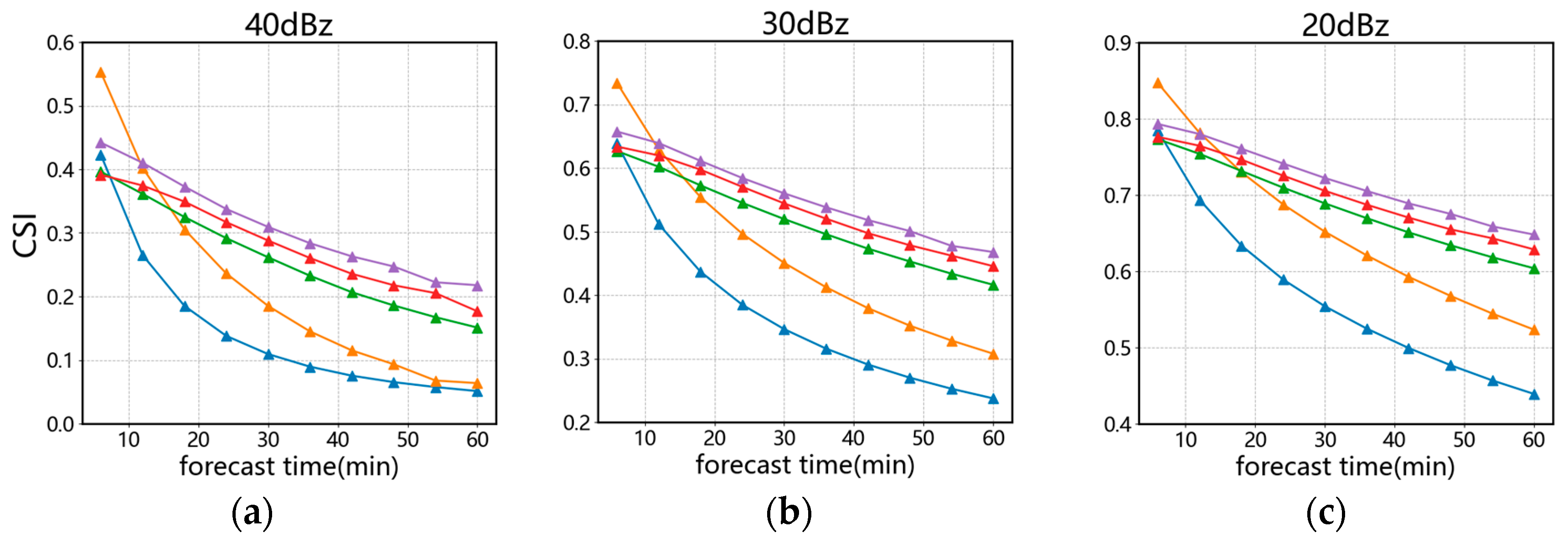
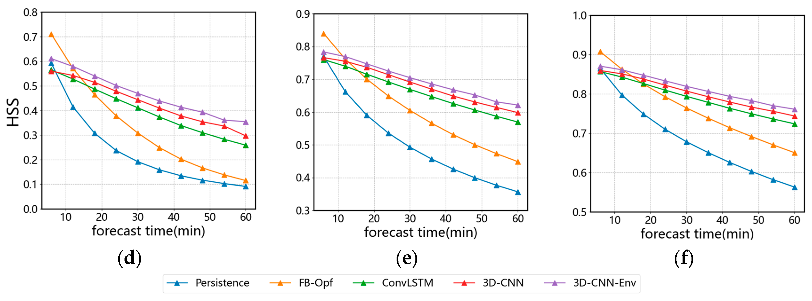
In addition to comparing models adding different environment fields, there are some relevant contrast experiments: the Farenback optical flow method (FB-Opf), constant extrapolation (Persistence), ConvLSTM, and 3D-CNN extrapolation without environment field (3D-CNN). Since the best results are obtained by adding the divergence field, we use the model with the divergence field as the representative model for our method (3D-CNN-Env). The average results over all moments with different thresholds are shown in

Table 5. Test results of different extrapolation methods.

Threshold	Method	POD↑	FAR↓	CSI↑	ETS↑	HSS↑
20dBZ	FB-Opf	0.7760	0.2006	0.6495	0.6157	0.7622
	ConvLSTM	0.8035	0.1813	0.6821	0.6506	0.7883
	3D-CNN	0.8102	0.1655	0.6980	0.6680	0.8009
	3D-CNN-ENV	0.8372	0.1675	0.7165	0.6874	0.8147
30dBZ	FB-Opf	0.6075	0.3552	0.4552	0.4383	0.6095
	ConvLSTM	0.7005	0.3460	0.5111	0.4943	0.6616
	3D-CNN	0.7142	0.3238	0.5322	0.5160	0.6807
	3D-CNN-ENV	0.7423	0.3114	0.5557	0.5399	0.7012
40dBZ	FB-Opf	0.3056	0.6028	0.2088	0.2060	0.3416
	ConvLSTM	0.3886	0.5613	0.2595	0.2566	0.4084
	3D-CNN	0.3972	0.5157	0.2791	0.2763	0.4330
	3D-CNN-ENV	0.4445	0.4851	0.3133	0.3104	0.4738

. The runtime costs are shown in

Table 6. The runtime costs of different networks.

Model	Video Memory for Training	Calulation Time (GPU)
3D-CNN	12.89 GB (Batch size = 8)	0.0032 s
3D-CNN-ENV	13.42 GB (Batch size = 8)	0.0034 s
ConvLSTM	18.34 GB (Batch size = 4)	0.0031 s

.

It is shown that the 3D-CNN neural network can significantly improve the extrapolation quality compared with the traditional optical flow method and ConvLSTM. The introduction of environment fields further enhances the prediction capability of the neural network. Table 6 shows that the calculation times of the three models are nearly the same. The introduction of the environment field only increases the computation of the original model by a very small amount.

More detailed evaluation results are shown in Figure 5. Each graph represents the trend of CSI or HSS scores with an increase in lead time. It can be seen that: (1) as the lead time increases, the CSI and HSS scores of the five models invariably show a decreasing trend. The score of the optical flow method and constant extrapolation decreased significantly more than 3D-CNN and ConvLSTM models. (2) The optical flow method performs best at the first prediction moment (6 min) and is on par with the best overall performing 3D-CNN-Env model at the second prediction moment (12 min), but then it declines rapidly all the way down. (3) Among the four extrapolation models without environment fields, the 3D-CNN model shows the best performance, the ConvLSTM model is the second best, and the constant extrapolation is the worst. (4) Compared to the best-performing 3D-CNN model, the introduction of the environment field improves the score by 2%.

3.3. Convective Cell Level Test

3.3.1. Convective Cell Level Evaluation Indicators

The prediction can be categorized as a classification problem for metrics design according to the definition of a storm cell’s evolution. Besides the pixel-level-based test method, we also designed a storm cell-based test method to verify the model’s ability to predict the status of storm cells and their generation and extinction in the future. We use the principle of nearest center-of-mass distance to match cells in different images. Therefore, we use the Hungarian algorithm [41], which is a combinatorial optimization algorithm suitable for solving the minimum distance matching problem. We calculate a distance matrix between the centers of mass. The Hungarian algorithm can find a unique solution to minimize the sum of the distances of matched center-of-mass pairs. This provides information on whether the convective cells output by the radar extrapolation model match the convective cells of real radar images.

The specific testing steps are as follows:

Step 1: Segment the strong storm cells over 40 dBZ from the image.

Step 2: Reserve the cells that are greater than 30 pixel points.

Step 3: Calculate the centroid position of each cell.

Step 4: Calculate the distance between the centroid in the predicted image and the centroid in the observed image to get the distance matrix d.

Step 5: Use the Hungarian algorithm to match the centroids from the predicted image and the observed image one by one. If the distance between the two centroids after matching is greater than 20 km, the matching is invalidated.

Step 6: A successful match is considered a true positive (TP), a centroid that is not matched in the observed image is considered a false negative (FN), and a centroid that is not matched in the predicted image is considered a false positive (FP).

Step 7: Calculate the probability of detection (POD), false alarm ratio (FAR), and critical success index (CSI) based on the number of true positives, false negatives, and false positives.

3.3.2. Convective Cell Level Test Results

The test results based on the storm cells according to the method in Section 3.3.1 are shown in

Table 7. Test results based on the storm cell’s centroid distance match method.

Method	POD↑	FAR↓	CSI↑
3D-CNN	0.5262	0.3774	0.3989
Persistence	0.4978	0.6048	0.2824
FB-Opf	0.5516	0.4684	0.3712
ConvLSTM	0.5191	0.3914	0.3892
3D + Divergence	0.5711	0.3273	0.4469
3D + Vertical Velocity	0.5157	0.3384	0.4081
3D + Vorticity	0.4650	0.3215	0.3810
3D + Geopotential Height	0.4932	0.3135	0.4026
3D + Relative Humidity	0.5772	0.4010	0.4163
3D + Specific Humidity	0.5544	0.3688	0.4187
3D + Temperature	0.5135	0.3498	0.4023
3D + Dynamic	0.5169	0.3185	0.4164
3D + Humidity	0.5357	0.3755	0.4052
3D + Dynamic and humidity	0.5486	0.3379	0.4286
3D + Dynamic and temperature	0.5460	0.3259	0.4320
3D + Humidity and temperature	0.5265	0.3636	0.4048
3D + All Environment Fields	0.5294	0.3590	0.4083

. Compared with the pixel-level test method, the method based on the matching of the centroid distance of storm cells reflects the model’s power for predicting the formation of newborn cells and the extinction of old cells. Table 7 shows that adding the environment fields can also show significant advantages at the storm cell level, such as divergence, humidity, and the combination of dynamics and temperature, which can achieve better enhancement effects.

4. Case Analysis

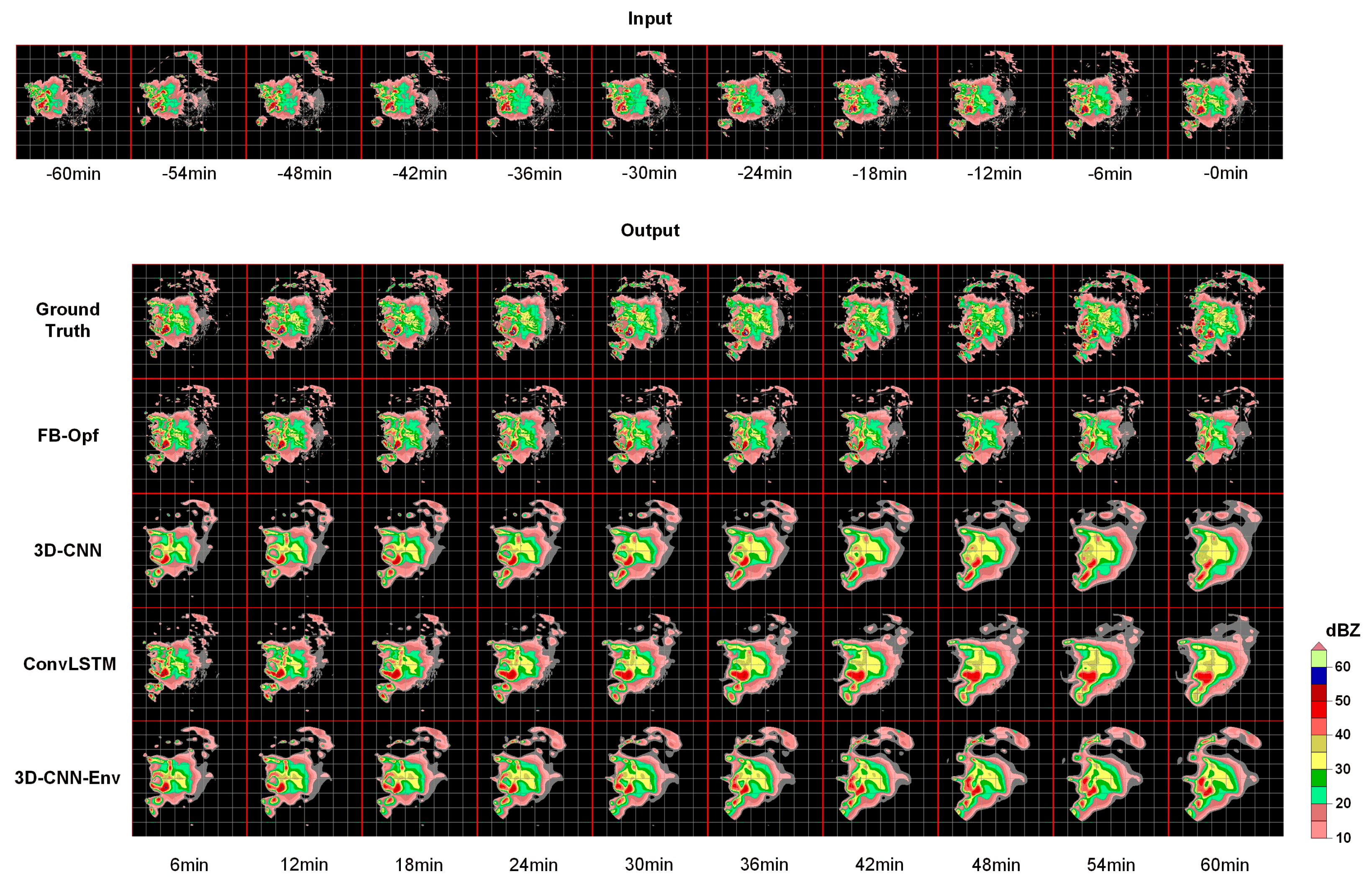
In order to visually evaluate the improvement of the environment field on the radar echo extrapolation, we chose two cases to illustrate it. Figure 6 shows a visual comparison of the radar echo sequence observed at Bingzhou station on 13 June 2016 at 8:06–9:00 and the results obtained from the three extrapolation models. The model inputs are all the observed sequences on 13 June 2016 at 7:00–8:00.

As can be seen from the top row of Figure 6, the lower left region at the beginning of the observed image sequence contains a larger convective cell as well as several scattered smaller convective cells. As the lead time increases, the large convective cell tends to be stable, while numerous small convective cells converge. A new large convective cell and a strong small convective cell are formed on the left and lower left sides of the stable cell at about 54 min. In addition, the reflectivity in the upper left area is gradually increasing. The optical flow method has excellent prediction in the first few moments, but the prediction of the large convective cell shows significant deformation and scale decay. It fails to predict the new large cell’s generation by the merging of the small cells. In contrast, for the 3D-CNN model without the inclusion of the environment field, it is able to predict the motion trend of the cell and maintain its shape roughly, but the model tends to predict more and more ambiguous images. The model predicts that the scattered small cells around the large cell will gradually die out in the future, thus failing to successfully predict the generation of new large cells on the left. ConvLSTM performs well in predicting the first three images but soon tends to predict ambiguous results. It fails to predict the trend of echo enhancement in the upper left of the image, and the cells in the middle lack detail. After introducing the divergence field to the 3D model, it successfully predicts the generation of new cells on the left and lower left sides and the enhancement of reflectivity in the upper left region with the assistance of the divergence field, although it still outputs an ambiguity prediction.

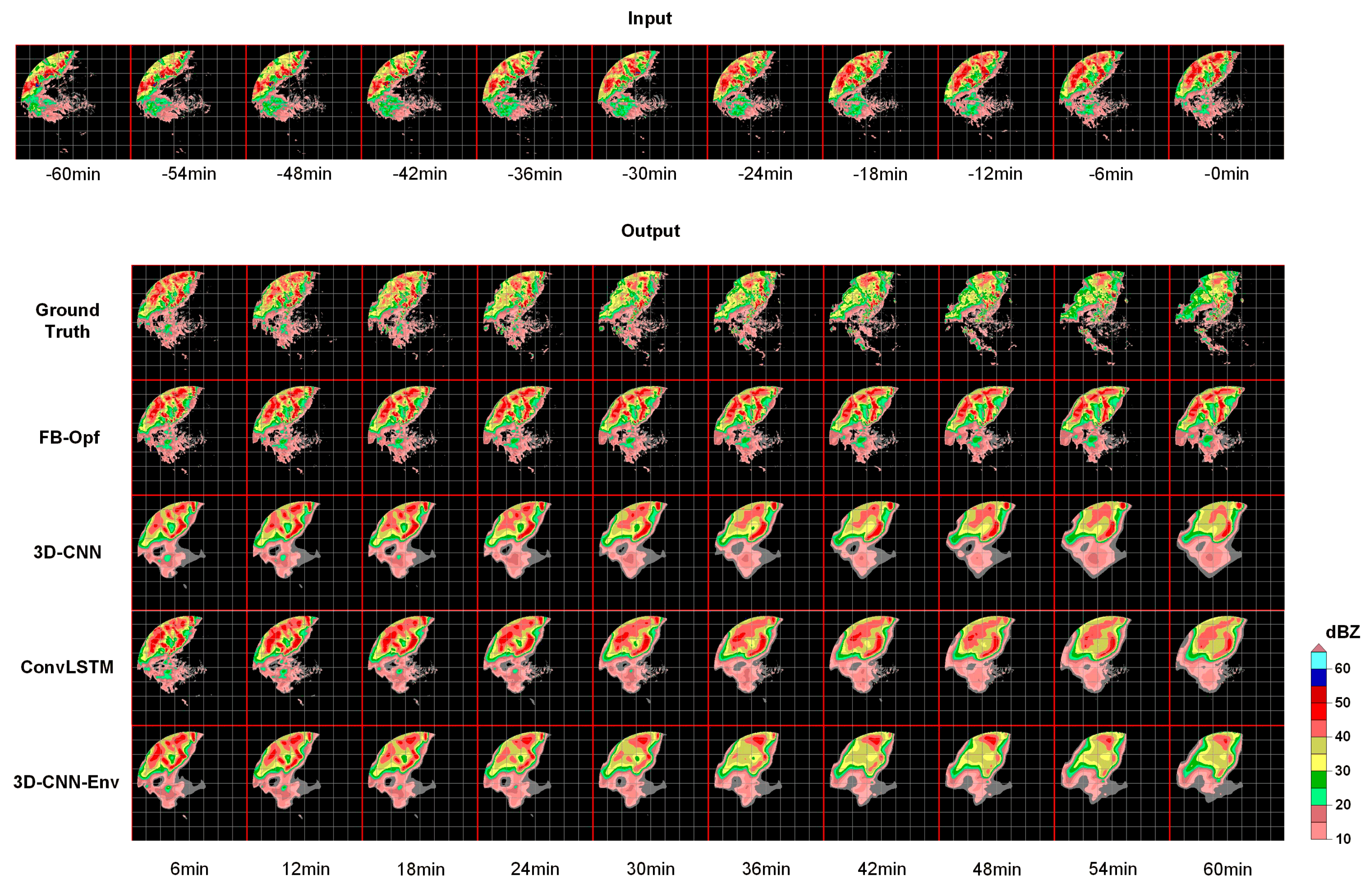
The second case shows a visual comparison of the radar echo sequence observed in Yantai station on 30 July 2016 at 14:06–15:00 and the results obtained from the three extrapolation models. The model inputs are all the observed sequences on 30 July 2016 at 13:00–14:00.

The ground truth of Figure 7 shows that the upper left region at the beginning of the observed image sequence contains multiple strong convective cells of varying sizes. As the lead time increases, the left cells gradually die out, and the right cells gradually evolve into a cluster and a band (24 min). Then, the upper side of the band echo merges with its left cell, while its lower side splits from the main body to form a separate cell (36 min). The two merged and split convective regions then enter into a weakening process. Finally, most cells are dead, leaving a few small, scattered cells. Since the optical flow method cannot predict the variation of the reflectivity, the radar reflectivity in row two remains essentially constant throughout the predicted sequence, which leads to a false prediction of the evolutionary processes of extinction, merger, and splitting of the cell. For the 3D-CNN model without environmental field and the ConvLSTM model, the radar echo starts to fade at about 36 min, but there is still a strong convective cell at the center of the image until 60 min. The information provided by the divergence field helps the model predict the weakening of the strong convective region at 24 min and correctly predict the extinction of the left cell, the merging and splitting of the band echo, and the clump echo.

In this article, a visualization method similar to Figure 5 and Figure 6 was used to analyze and compare all 1589 test samples. Approximately 10% of samples had generation, extinction, merging, and splitting in the 1-h echo evolution. Most of them gave similar optimistic predictions, similar to the examples in Figure 5 and Figure 6, fully illustrating that the inclusion of environmental fields has a positive constraint and guiding effect on the radar echo prediction.

5. Conclusions

In this paper, we propose a 3D convolutional neural network combing both radar and environmental field information to improve extrapolation performance. Our main contributions are: (1) By interpolation in the temporal dimension and down-sampling in the spatial dimension, the adaptation of the environmental field and radar echo sequence in spatial and temporal resolution is obtained. (2) The structure of the two kinds of encoders realizes the fusion of the two inputs in the channel dimension. They jointly participate in the extrapolation proceeding. (3) We explored the influence of different environmental fields and their combinations on predicting radar echoes. Finally, we conclude that the divergence field performs best in improving radar echo extrapolation quality.

Several experiments demonstrate the advantages of the proposed model in this paper: On the pixel level, the CSI of the 3D CNN model after introducing the divergence field is improved by 10% compared with the conventional optical flow method and by 2%–3% compared with the 3D CNN model without the environment field. On the convective cell level, the CSI is improved by 7.6% compared with the optical flow method and by 4.8% compared with the 3D CNN model without the environment field. Two cases show the capability of predicting the generation, extinction, merger, and splitting of convective cells. Therefore, we can conclude that using environment field information can improve extrapolation performance.

The experiments demonstrated that multi-source data provide more reliable information for radar extrapolation. Since the environment field provides information on the evolution of convective systems, we expect to further extend the effective time of extrapolation to two hours or even longer. Our future work will focus on building more complex models considering the structure of typical weather systems based on environmental information and meteorological knowledge, which fuse the environmental fields and radar data more effectively for better extrapolation performance.

References

1. Wilson, J.W.; Ebert, E.; Saxen, T.R.; Roberts, R.D.; Mueller, C.K.; Sleigh, M.; Pierce, C.E.; Seed, A. Sydney 2000 Forecast Demonstration Project: Convective Storm Nowcasting. Weather Forecast. 2004, 19, 131–150. [Google Scholar] [CrossRef]
2. Bauer, P.; Thorpe, A.; Brunet, G. The quiet revolution of numerical weather prediction. Nature 2015, 525, 47–55. [Google Scholar] [CrossRef] [PubMed]
3. Sun, J.; Xue, M.; Wilson, J.W.; Zawadzki, I.; Ballard, S.P.; Onvlee-Hooimeyer, J.; Joe, P.; Barker, D.; Li, P.-W.; Golding, B.; et al. Use of NWP for Nowcasting Convective Precipitation: Recent Progress and Challenges. Bull. Am. Meteorol. Soc. 2014, 95, 409–426. [Google Scholar] [CrossRef] [Green Version]
4. Prudden, R.; Adams, S.; Kangin, D.; Robinson, N.; Ravuri, S.; Mohamed, S.; Arribas, A. A Review of Radar-Based Nowcasting of Precipitation and Applicable Machine Learning Techniques. arXiv 2020, arXiv:2005.04988. [Google Scholar]
5. Johnson, J.T.; Mackeen, P.L.; Witt, A.; Mitchell, E.D.W.; Stumpf, G.J.; Eilts, M.D.; Thomas, K.W. The Storm Cell Identification and Tracking Algorithm: An Enhanced WSR-88D Algorithm. Weather Forecast. 1998, 13, 263–276. [Google Scholar] [CrossRef]
6. Dixon, M.; Wiener, G. TITAN: Thunderstorm Identification, Tracking, Analysis, and Nowcasting—A Radar-Based Methodology. J. Atmos. Ocean. Technol. 1993, 10, 785–797. [Google Scholar] [CrossRef]
7. Rinehart, R.E.; Garvey, E.T. Three-dimensional storm motion detection by conventional weather radar. Nature 1978, 273, 287–289. [Google Scholar] [CrossRef]
8. Bowler, N.; Pierce, C.E.; Seed, A. Development of a precipitation nowcasting algorithm based upon optical flow techniques. J. Hydrol. 2004, 288, 74–91. [Google Scholar] [CrossRef]
9. Woo, W.-C.; Wong, W.-K. Operational Application of Optical Flow Techniques to Radar-Based Rainfall Nowcasting. Atmosphere 2017, 8, 48. [Google Scholar] [CrossRef] [Green Version]
10. Ayzel, G.; Heistermann, M.; Winterrath, T. Optical flow models as an open benchmark for radar-based precipitation nowcasting (rainymotion v0.1). Geosci. Model Dev. 2019, 12, 1387–1402. [Google Scholar] [CrossRef] [Green Version]
11. Huang, X.; Ma, Y.; Hu, S. Extrapolation and effect analysis of weather radar echo sequence based on deep learning. Acta Meteorol. Sin. 2021, 79, 817–827. [Google Scholar] [CrossRef]
12. Shi, X.; Chen, Z.; Wang, H.; Yeung, D.-Y.; Wong, W.-K.; Woo, W.-C. Convolutional LSTM network: A machine learning approach for precipitation nowcasting. In Proceedings of the Advances in Neural Information Processing Systems (NeurIPS), Montreal, QC, Canada, 7–12 December 2015; pp. 802–810. [Google Scholar] [CrossRef] [Green Version]
13. Shi, X.; Gao, Z.; Lausen, L.; Wang, H.; Yeung, D.-Y.; Wong, W.-K.; Woo, W.-C. Deep learning for precipitation nowcasting: A benchmark and a new model. In Proceedings of the Advances in Neural Information Processing Systems (NeurIPS), Long Beach, CA, USA, 4–9 December 2017; pp. 5618–5628. [Google Scholar]
14. Wang, Y.; Long, M.; Wang, J.; Gao, Z.; Yu, P.S. PredRNN: Recurrent neural networks for predictive learning using spatiotemporal lstms. In Proceedings of the Advances in Neural Information Processing Systems (NeurIPS), Long Beach, CA, USA, 4–9 December 2017; pp. 879–888. [Google Scholar]
15. Wang, Y.; Gao, Z.; Long, M.; Wang, J.; Yu, P.S. PredRNN++: Towards a resolution of the deep-in-time dilemma in spatiotemporal predictive learning. In Proceedings of the Advances in the 35th International Conference on Machine Learning (ICML), Stockholm, Sweden, 10–15 July 2018; pp. 5123–5132. [Google Scholar]
16. Wang, Y.; Zhang, J.; Zhu, H.; Long, M.; Wang, J.; Yu, P.S. Memory in memory: A predictive neural network for learning higher-order non-stationarity from spatiotemporal dynamics. In Proceedings of the IEEE Conference on Computer Vision and Pattern Recognition, Long Beach, CA, USA, 16–20 June 2019; pp. 9154–9162. [Google Scholar] [CrossRef] [Green Version]
17. Agrawal, S.; Barrington, L.; Bromberg, C.; Burge, J.; Gazen, C.; Hickey, J. Machine learning for precipitation nowcasting from radar images. In Proceedings of the Advances in Neural Information Processing Systems (NeurIPS), Vancouver, BC, Canada, 8–14 December 2019; p. 4. [Google Scholar]
18. Kim, D.-K.; Suezawa, T.; Mega, T.; Kikuchi, H.; Yoshikawa, E.; Baron, P.; Ushio, T. Improving precipitation nowcasting using a three-dimensional convolutional neural network model from Multi Parameter Phased Array Weather Radar observations. Atmos. Res. 2021, 262, 105774. [Google Scholar] [CrossRef]
19. Klein, B.; Wolf, L.; Afek, Y. A Dynamic Convolutional Layer for short range weather prediction. In Proceedings of the IEEE Conference on Computer Vision and Pattern Recognition (CVPR), Boston, MA, USA, 8–10 June 2015; pp. 4840–4848. [Google Scholar]
20. Wang, C.; Wang, P.; Wang, P.P.; Xue, B.; Wang, D. Using Conditional Generative Adversarial 3-D Convolutional Neural Network for Precise radar extrapolation. IEEE J. Sel. Top. Appl. Earth Obs. Remote Sens. 2021, 14, 5735–5749. [Google Scholar] [CrossRef]
21. Wu, H.; Yao, Z.; Wang, J.; Long, M. MotionRNN: A flexible model for video prediction with spacetime-varying motions. In Proceedings of the IEEE/CVF Conference on Computer Vision and Pattern Recognition (CVPR), Kuala Lumpur, Malaysia, 18–20 December 2021; pp. 15435–15444. [Google Scholar]
22. Han, L.; Liang, H.; Chen, H.; Zhang, W.; Ge, Y. Convective Precipitation Nowcasting Using U-net Model. IEEE Trans. Geosci. Remote Sens. 2022, 60, 4103508. [Google Scholar] [CrossRef]
23. Yu, X.; Yao, X.; Xiong, Y.; Zhou, X.; Wu, H.; Deng, B.; Song, Y. Principle and Operational Application of Doppler Weather Radar; China Meteorological Press: Beijing, China, 2006; pp. 92–95. ISBN 978-7-5029-4111-6.
24. Wilson, J.W.; Crook, N.A.; Mueller, C.K.; Sun, J.; Dixon, M. Nowcasting Thunderstorms: A Status Report. Bull. Am. Meteorol. Soc. 1998, 79, 2079–2100. [Google Scholar] [CrossRef]
25. Pulkkinen, S.; Nerini, D.; Pérez Hortal, A.A.P.; Velasco-Forero, C.; Seed, A.; Germann, U.; Foresti, L. Pysteps: An open-source Python library for probabilistic precipitation nowcasting (v1.0). Geosci. Model Dev. 2019, 12, 4185–4219. [Google Scholar] [CrossRef] [Green Version]
26. Sokol, Z. Assimilation of extrapolated radar reflectivity into a NWP model and its impact on a precipitation forecast at high resolution. Atmos. Res. 2011, 100, 201–212. [Google Scholar] [CrossRef]
27. Wang, G.; Wong, W.-K.; Hong, Y.; Liu, L.; Dong, J.; Xue, M. Improvement of forecast skill for severe weather by merging radar-based extrapolation and storm-scale NWP corrected forecast. Atmos. Res. 2015, 154, 14–24. [Google Scholar] [CrossRef]
28. Pan, X.; Lu, Y.; Zhao, K.; Huang, H.; Wang, M.; Chen, H. Improving Nowcasting of Convective Development by Incorporating Polarimetric Radar Variables into a Deep-Learning Model. Geophys. Res. Lett. 2021, 48, e2021GL095302. [Google Scholar] [CrossRef]
29. Klocek, S.; Dong, H.; Dixon, M.; Kanengoni, P.; Kazmi, N.; Luferenko, P.; Lv, Z.; Sharma, S.; Weyn, J.; Xiang, S. MS-nowcasting: Operational Precipitation Nowcasting with Convolutional LSTMs at Microsoft Weather. arXiv 2021, arXiv:2111.09954. [Google Scholar]
30. Min, C.; Chen, S.; Gourley, J.J.; Chen, H.; Zhang, A.; Huang, Y.; Huang, C. Coverage of China New Generation Weather Radar Network. Adv. Meteorol. 2019, 2019, 5789358. [Google Scholar] [CrossRef]
31. Zhong, L.; Zhang, Z.; Chen, L.; Yang, J.; Zou, F. Application of the Doppler weather radar in real-time quality control of hourly gauge precipitation in eastern China. Atmos. Res. 2016, 172–173, 109–118. [Google Scholar] [CrossRef] [Green Version]
32. Hersbach, H.; Bell, B.; Berrisford, P.; Hirahara, S.; Horányi, A.; Muñoz-Sabater, J.; Nicolas, J.; Peubey, C.; Radu, R.; Schepers, D.; et al. The ERA5 global reanalysis. Q. J. R. Meteorol. Soc. 2020, 146, 1999–2049. [Google Scholar] [CrossRef]
33. Weisman, M.L.; Klemp, J.B. Characteristics of Isolated Convective Storms. In Mesoscale Meteorology and Forecasting; American Meteorological Society: Boston, MA, USA, 1986; pp. 331–358. [Google Scholar]
34. Tran, D.; Bourdev, L.; Fergus, R.; Torresani, L.; Paluri, M. Learning spatiotemporal features with 3D convolutional networks. In Proceedings of the IEEE International Conference on Computer Vision (ICCV), Santiago, Chile, 13–16 December 2015; pp. 4489–4497. [Google Scholar]
35. Snoek, C.G.; Worring, M.; Smeulders, A.W. Early versus late fusion in semantic video analysis. In Proceedings of the 13th Annual ACM International Conference on Multimedia, Singapore, 6–11 November 2005; pp. 399–402. [Google Scholar] [CrossRef]
36. Ioffe, S.; Szegedy, C. Batch normalization: Accelerating deep network training by reducing internal covariate shift. In Proceedings of the 32nd International Conference on Machine Learning (ICML), Lille, France, 6–11 July 2015; pp. 448–456. [Google Scholar]
37. Dubey, S.R.; Singh, S.K.; Chaudhuri, B.B. Activation functions in deep learning: A comprehensive survey and benchmark. Neurocomputing 2022, 503, 92–108. [Google Scholar] [CrossRef]
38. Luo, Y.; Zhao, W.; Zhai, J. Dichotomous weather forecasts score research and a new measure of score. J. Appl. Meteorol. Sci. 2009, 2, 129–136. [Google Scholar]
39. Donaldson, R.J.; Dyer, R.M.; Kraus, M.J. An objective evaluator of techniques for predicting severe weather events. In Proceedings of the 9th Conference on Severe Local Storms, Norman, OK, USA, 21–23 October 1975; pp. 321–326. [Google Scholar]
40. Black, T.L. The New NMC Mesoscale Eta Model: Description and Forecast Examples. Weather. Forecast. 1994, 9, 265–278. [Google Scholar] [CrossRef]
41. Kuhn, H.W. The Hungarian method for the assignment problem. Nav. Res. Logist. Q. 1955, 2, 83–97. [Google Scholar] [CrossRef] [Green Version]
Figure 1. Radar data coverage area.
Atmosphere 14 00980 g001
Figure 2. Schematic diagram of an extrapolation sample.
Atmosphere 14 00980 g002
Figure 3. Schematic diagram of two convolution operations: (a) 2D convolution; (b) 3D convolution.
Atmosphere 14 00980 g003
Figure 4. Structure of extrapolation model.
Atmosphere 14 00980 g004
Figure 5. Subfigures(af) present the CSI and HSS scores of five extrapolation methods at different lead times and thresholds.
Atmosphere 14 00980 g005aAtmosphere 14 00980 g005b
Figure 6. Visualization of an extrapolation case in Bingzhou on 13 June 2016, 07:00−09:00.
Atmosphere 14 00980 g006
Figure 7. Visualization of an extrapolation case in Yantai on 30 July 2016, 13:00−15:00.
Atmosphere 14 00980 g007