Wave and Meso-Scale Eddy Climate in the Arctic Ocean

Abstract

Under global climate change, the characteristics of oceanic dynamics are gradually beginning to change due to melting sea ice. This study focused on inter-annual variation in waves and mesoscale eddies (radius > 40 km) in the Arctic Ocean from 1993 to 2021. The waves were simulated by a numerical wave model, WAVEWATCH-III (WW3), which included a parameterization of ice–wave interaction. The long-term wind data were from the European Centre for Medium-Range Weather Forecasts (ECMWF) reanalysis (ERA-5), and current and sea level data from the HYbrid Coordinate Ocean Model (HYCOM)were used as the forcing fields. The simulated significant wave heights (SWHs) were validated against the 2012 measurements from the Jason-2 altimeter, yielding a 0.55 m root mean square error (RMSE) with a 0.95 correlation (COR). The seasonal variation in WW3-simulated SWH from 2021 to 2022 showed that the SWH was the lowest in summer (July and August 2021) and highest in winter (November 2021 to April 2022). This result indicates that parts of the Arctic could become navigable in summer. The mesoscale eddies were identified using a daily-averaged sea level anomalies (SLA) product with a spatial resolution of a 0.25° grid for 1993−2021. We found that the activity intensity (EKE) and radius of mesoscale eddies in the spatial distribution behaved in opposing ways. The analysis of seasonal variation showed that the increase in eddy activity could lead to wave growth. The amplitude of SWH peaks was reduced when the Arctic Oscillation Index (AOI) was <−1.0 and increased when the AOI was >0.5, especially in the case of swells. The amplitude of SWH oscillation was low, and the EKE and radius of eddies were relatively small. Although the radius and EKE of eddies were almost similar to the AOI, the waves also influenced the eddies.

1. Introduction

The sea ice in the Arctic Ocean has been gradually melting since the previous century due to global warming [1]. With the sea fetch enlarging [2,3] and sea levels rising [4], marine dynamics is an important field, especially the study of waves [5] and currents [6]. Traditionally, research on atmospheric–marine processes relies on data from field observations, such as those collected by annual scientific expeditions to the North Pole by the Chinese ship Xuelong. However, ship-based data cannot be used for long-term analysis.

Because of improvements in computational technology and advances in oceanography, numerical modeling for marine prediction is well-developed [7]. Typically, several models are used for various dynamics, i.e., Simulating Waves Nearshore (SWAN) and WAVEWATCH-III (WW3) for waves [8,9], Finite-Volume Community Ocean Model (FVCOM) and HYbrid Coordinate Ocean Model (HYCOM) for tides and currents [10,11], and non-hydrostatic numerical models for internal waves [12]. Currently, two numerical wave models following the basic principles of the third-generation ocean wave model (WAM) [13] are commonly used for research on hindcasting waves [14], especially at extreme sea states, i.e., tropical cyclones [15,16] and in polar oceans [17]. The SWAN, which has a triangular mesh, was initially developed by the Delft University of Technology [18,19] for wave simulation in complicated coastal waters. The WW3 model uses rectangular grids and is usually employed for simulating waves over global oceans [20,21]. The newly released versions of SWAN (41.41) and WW3 (6.07) use alternate meshes, i.e., unstructured, and structured grids. The parameterization of ice–wave interactions is provided by the WW3 model [22,23,24], i.e., the pure viscous layer model [25], elastic plate model [26], viscoelastic model [27], and thin-elastic-plate scattering model [28]. These parameterizations were developed based on observations from various seas in the Arctic Ocean. The WW3 model has been used to study wave propagation through ice cover in the Arctic Ocean [29], even in stormy conditions [30]. Therefore, the wave climate in the Arctic Ocean could be studied through the long-term variation in modeled waves.

Several remote-sensing techniques, i.e., scatterometer [31], altimeter [32], synthetic aperture radar (SAR) [33], and the Chinese–French Oceanic SATellite (CFOSAT) [34], have capabilities for global wind and wave monitoring. Altimeters launched since the 1990s, i.e., Jason-1/2/3, can measure sea level anomalies (SLA) [35]. If we assume that the geostrophic current is correlated with the geostrophic velocity anomaly field, mesoscale eddies can be detected using SLA data [36,37,38]. Recent work has revealed that SLA data are a valuable resource for research on the evolution of meso-scale eddies at moderate latitudes. However, eddies at a scale of <~40 km are rarely observed by altimeters due to the coarse spatial resolution of altimeter-based SLA data with a 0.25° grid. In the literature, the current speed is directly related to the Coriolis force, which is inversely proportional to latitude. Therefore, mesoscale eddies are also detectable in polar regions, although the eddies’ activity intensity (EKE) is relatively weak.

Climate change causes sea fetch enlargement, thus increasing wave forcing by the strong wind stress in the Arctic Ocean. In addition, mesoscale eddies respond to extreme events (El Niño and La Niña) in the tropical Pacific Ocean [39] due to atmospheric circulation between the equator and the polar regions. The wave climate is usually studied using wave product altimeter data. However, the wave climate associated with the variation in mesoscale eddies needs further analysis. In this study, we simulated wave distribution using the WW3 model, incorporating current–wave interactions [40], ice–wave interactions [2], and sea level rise [41]. The meso-scale eddies were identified using AVISO SLA data.

The remainder of this paper is structured as follows: Section 2 contains a discussion of the settings of the WW3 model, the forcing fields for the wave modeling in the Arctic Ocean, and the method of mesoscale eddy (radius >40 km) identification using SLA data; Section 3 contains information on the variation in WW3-simulated wave distribution and mesoscale eddies from 1993 to 2021, with specific coverage of climate of wave and mesoscale eddies in the context of El Niño and La Niña events; and the conclusions are summarized in Section 4.

2. Materials and Methods

Here, we describe the WW3 model and hindcast wave simulation. The datasets for modeling waves include ERA-5 wind, HYbrid Coordinate Ocean Model (HYCOM) current, HYCOM sea level, Copernicus Marine Environment Monitoring Service (CMEMS) sea ice concentration, and CMEMS thickness. We also introduce the altimeter-based data for eddy identification, i.e., Haiyang-2B (HY-2B) significant wave height (SWH) and AVISO SLA data from the Centre National d′Etudes Spatiales (CNES).

2.1. Model Settings of WW3

The first numerical model used for hindcasting waves over global oceans was WAM. The principle of WAM is to solve the balance equation that describes the variation in wave energy during wave propagation. Both WW3 and SWAN follow a theoretical foundation that can be expressed as follows:

$$\frac{\partial E}{\partial t}+\nabla ·\left[\left(c_g+c\right)\times E\right]=F$$

(1)

where

$${F=F}_{\mathit{in}}{+F}_{\mathit{bot}}{+F}_{\mathit{nl}}{+F}_{\mathit{other}}$$

(2)

and E is the wave energy density; c_g and c represent the group velocity and phase velocity; $\nabla$ is the Hamiltonian operator; and F is the forces acting on the seawater particle. The sources of F include wave stress F_in, depth-induced friction F_bot, non-linear dissipation source associated with wave–wave interaction F_nl, and other terms F_other, i.e., current–wave interactions, ice–wave interactions, and wave breaking. In this study, the switch package illustrating the F_in and F_bot source terms, ST6, in the technique manual [42], was used in the modeling. The wave–wave interaction term F_nl was represented by the switch GMD2 package [43]. Switch FLD2 was used to represent wave breaking [44], switch TR1 for current–wave interactions [40], and switch IC4_M1 for ice–wave interactions [5].

2.2. Fields for Modeling Waves

The wind was the main force field in the wave simulation. At present, several reanalysis systems provide data for the wind field, i.e., the European Centre for Medium-Range Weather Forecasts (ECMWF) [45], the Cross Calibrated Multi-Platform (CCMP), and the Global Forecast System (GFS) by the National Centers for Environmental Prediction (NCEP). Among these datasets, ECMWF has continuously collected global wind data up to 85°N since 1979. The newest version is ECMWF reanalysis (ERA-5), with a 0.25° grid at 1 h intervals. This model is better than the 6-h CCMP and GFS. Therefore, we used the ERA-5 wind field in this study. The simulated region was 40−85° N, 0−360° E. The model was initialized on 1 January 1993 and terminated on 30 December 2021. Figure 1 depicts the wind map from ERA-5 at 18:00 UTC on 1 July 2015. The solid boundary and water depth (with a minimum value of 10 m) were derived from the General Bathymetry Chart of the Oceans (GEBCO) with a spatial resolution of 1 km.

As previously determined [10,40], the accuracy of model-simulated waves is improved when currents and sea level are included, especially in extreme states (i.e., tropical cyclones). Therefore, global current and sea level data were collected every 3 h from HYCOM at 1/12°. In addition, daily-averaged sea ice concentrations and thicknesses, with a spatial resolution of 1/12°, were obtained from the CMEMS. The above data were used as a forcing field. The spatial resolution of WW3 was a 0.25° grid (~25 km) at intervals of 30 min. Figure 2 show the HYCOM current and sea level maps at 18:00 UTC on 1 July 2015. The CMEMS sea ice concentration and thickness maps for July 2015 are shown in Figure 3.

2.3. Altimeter-Based Data

Global wind data measured by scatterometer, and wave data measured by the HY-2B altimeter are available from October 2018. Other altimeters [46], i.e., TOPEX/Poseidon and Jason-1/2/3, also provide wave measurements. However, the footprint (~10 km) of the HY-2B altimeter covers as far as 80° N, whereas the measurements from the Jason-2 altimeter only cover latitudes < 60° N. Therefore, the Geophysical Data Records (GDR) data from the HY-2B altimeter in 2019 were used to validate the WW3-simulated SWH. The time difference between the WW3-simulated SWHs and HY-2B values was within 15 min, and the distance difference was less than 5 km. Figure 4 shows the SWH map derived from the HY-2B altimeter during 15–18 July 2020. The validation of WW3-simulated SWH against the available measurements from the HY-2B altimeter in 2020−2021 showed that the root mean square error (RMSE) was 0.55 m with a 0.95 correlation (COR), as exhibited in Figure 5. Although there was a tendency of under-estimation that was probably caused by the ERA-5 wind, the simulation by the WW3 model was suitable for wave climate analysis.

The daily-averaged SLA fusion data from several altimeters, i.e., Cryosat-2, Jason-2, Sentinel-3A, and Haiyang-2A (HY-2A), were collected on a 0.25° grid for the Arctic Ocean. This open-access product can be accessed by AVISO from CNES, providing well-calibrated geophysical data for scientific research. Figure 6 shows an example map of AVISO SLA data for 8 January 2022, in which data are lacking at 70–80° N, 90° E–90° W, and at high latitudes > 80° N. Thus, eddies were undetectable in such regions.

2.4. Meso-Scale Eddy Identification

According to oceanographic theory, the geometric characteristics of the sea surface current field are generated by two-dimensional SLA data [47]. The relationship between the current and SLA fields H_a follows:

$$u=–\frac{g}{f}\frac{\partial \mathit{Ha}}{\partial y}$$

(3)

$$v=\frac{g}{f}\frac{\partial \mathit{Ha}}{\partial x}$$

(4)

where u and v represent the current speed at latitude x and longitude y, respectively; g is the gravity acceleration constant (=9.8 m²/s); and f is the Coriolis force constant, which is inversely proportional to latitude. The components of current are used to detect eddies with the vector geometry algorithm. The EKE is calculated by

$$EKE=\frac{1}{2}({\overline{u}}^2+{\overline{v}}^2)$$

(5)

Because of the coarse spatial resolution of AVISO SLA data (0.25° grid), only eddies with a radius greater than 40 km can be identified. Until now, no data have been available on eddies in the Arctic Ocean. Although the validation is not presented here, the applicability of this approach for identifying meso-scale eddies has been confirmed in several studies [48]. Specifically, the eddy center is defined by the point meeting the following terms:

(1)

The components of the current speed u and v on both sides of the eddy center have opposite signs, and their absolute value increases with movement away from the center.

(2)

The minimum velocity point within the selected range is defined as the indeterminacy eddy center.

(3)

The directions of the two adjacent velocity vectors around the eddy center have to be close to each other and located in the same or adjacent quadrants to ensure the same direction of rotation.

After the eddy center is defined, the eddy edge is determined as the contour of the outermost closed flow function around the eddy center. Finally, the radius of the eddy is defined as the average distance from the center to each point on the edge of the eddy.

A flowchart describing mesoscale eddy identification from daily-averaged SLA data is illustrated in Figure 7.

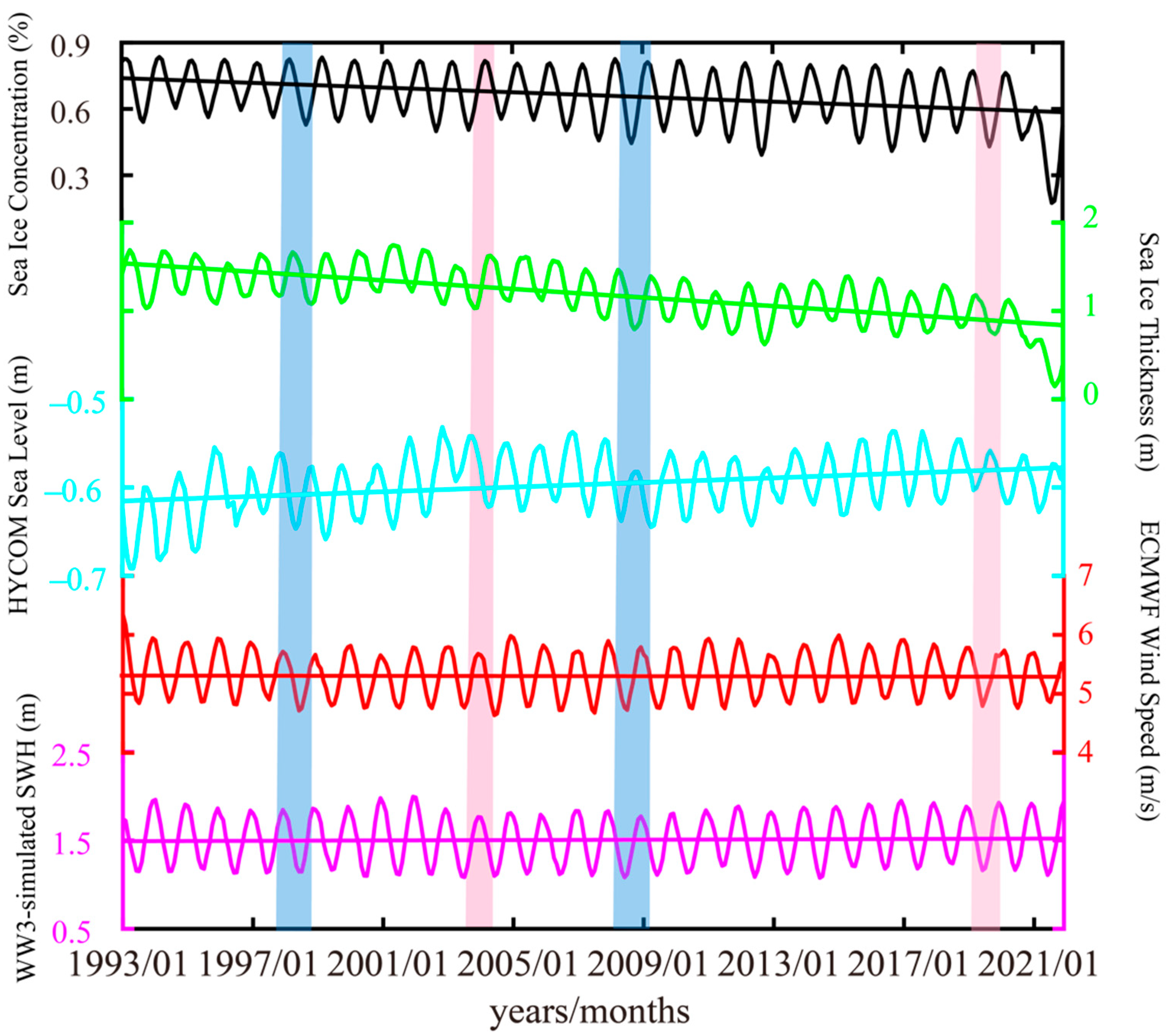
3. Results and Discussions

The WW3-simulated SWHs are validated against the HY-2B altimeter measurements in this section. The wave distribution in the Arctic Ocean is analyzed, and the long-term variation in meso-scale eddies is discussed.

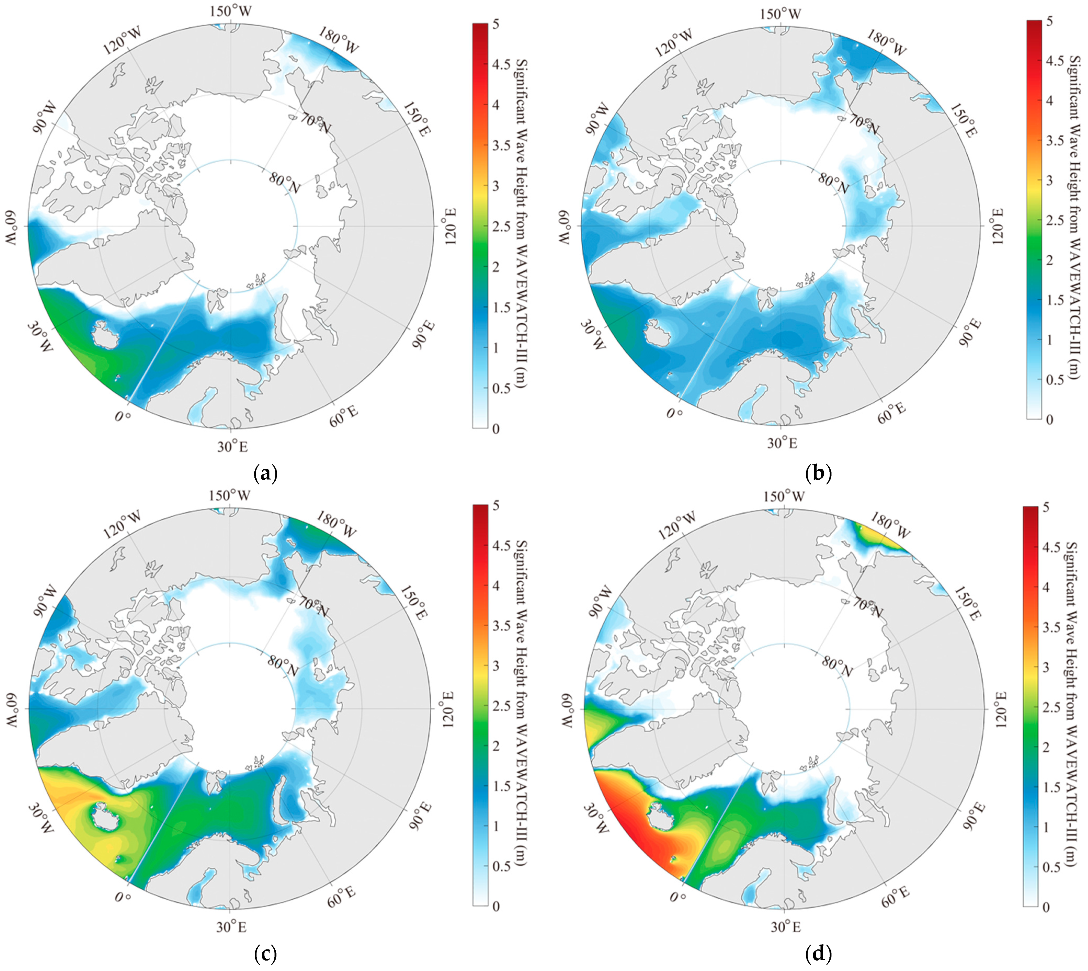
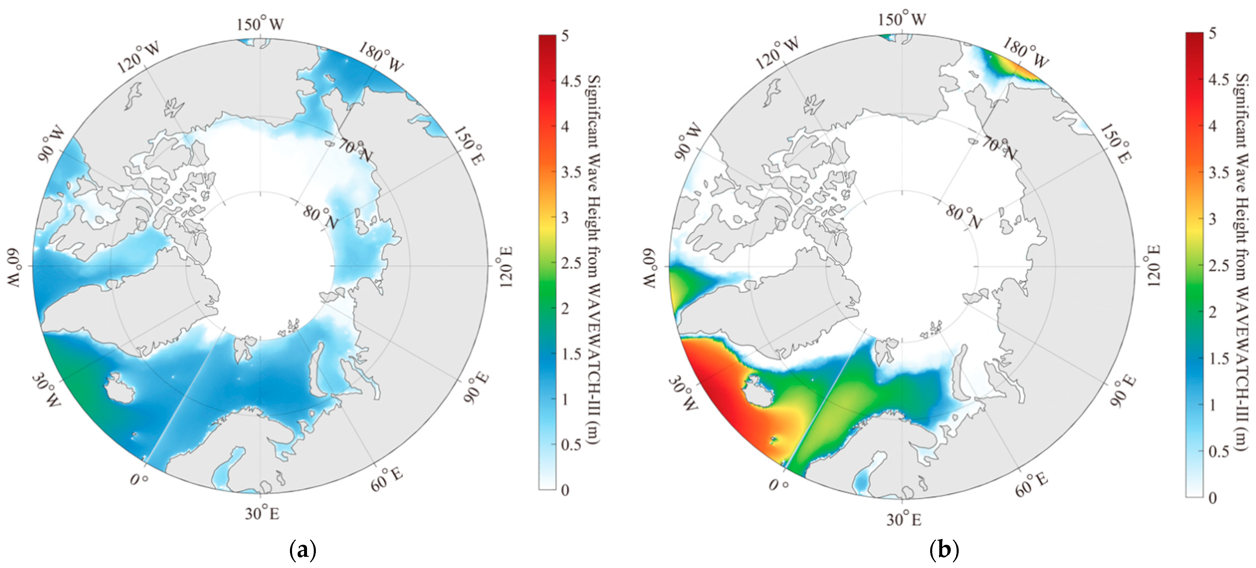
3.1. Wave Distribution

The variation in monthly averaged SWH simulated using the WW3 model is shown in Figure 8 according to the period (i.e., May and June 2021; July and August 2021; September and October 2021, and November 2021 to April 2022). We found that the SWHs were highest in winter, reaching up to 5 m. The wave intensity was lowest in summer (SWH < 2 m), probably caused by the weak winds during this season. This seasonal variation in SWH indicates that parts of the Arctic Ocean were more suitable for navigation in summer than in other seasons due to the reduction in sea ice and waves.

The long-term variation in ECMWF wind speed, HYCOM sea level, WW3-simulated SWH, CMEMS sea ice concentration, and sea ice thickness is presented in Figure 9. It is not surprising that the waves and wind have a similar oscillation trend over time because wave distribution is mainly determined by wind stress [5]. It can be observed that the sea ice thickness and concentration decreased overall, whereas the sea level increased overall. The synchronous changes in sea ice thickness and concentration were opposite the annual variations in winds, waves, and sea level (highlighted by blue bands in Figure 9). This was due to the increase in fetch associated with the reduction in sea ice. However, the sea level will likely vary negatively with wind and waves in certain years (highlighted by the pink bands in Figure 9). The correlation between waves and sea level is 0.32, and between waves and wind is 0.9. This indicates that the sea level weakly influences waves [10], although not as much as the wind. In the context of climate change, sea level rises gradually [49], and sea level anomalies are correlated with the distribution of meso-scale eddies [50]. Therefore, the climate of waves and meso-scale eddies needs further study.

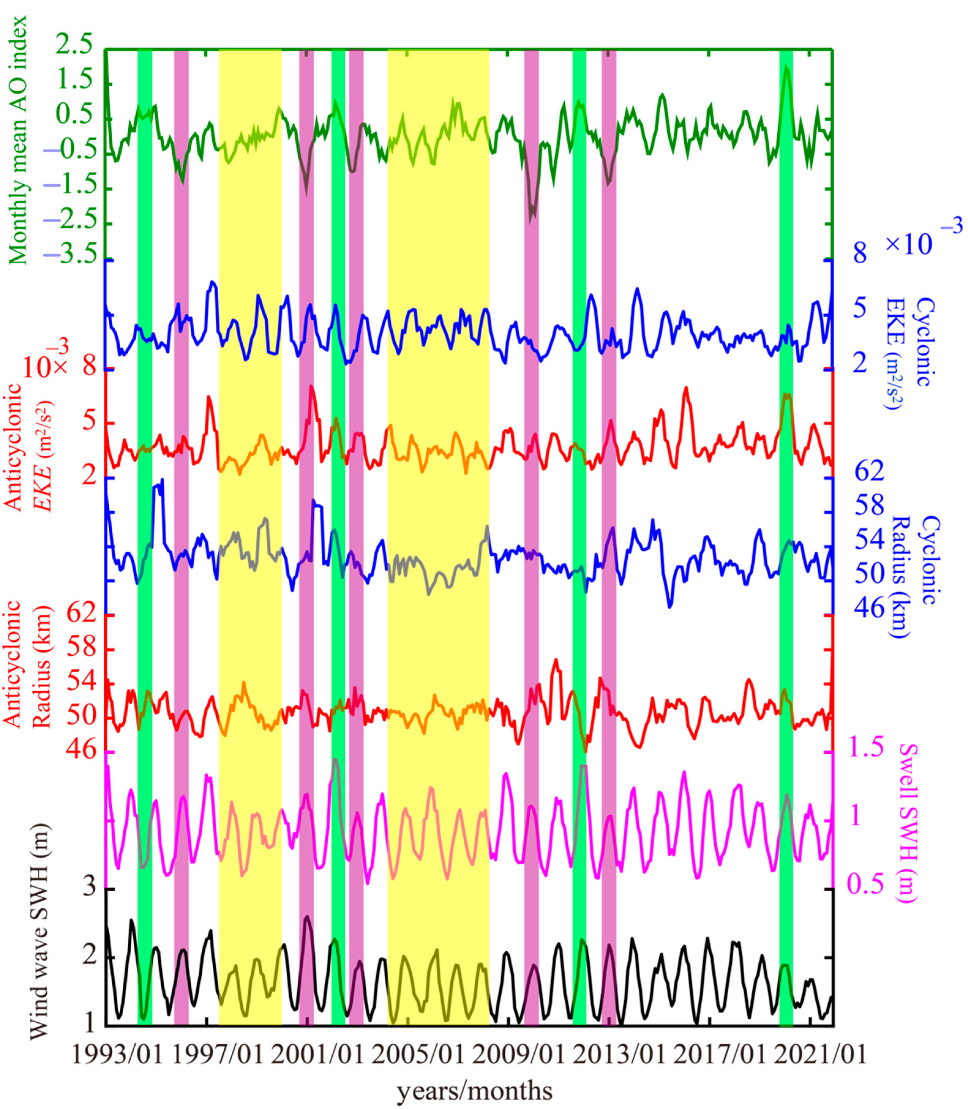
3.2. Variation in Meso-Scale Eddies

Figure 10a illustrates the detection of mesoscale eddies (radius r > 40 km) from SLA products for 7 September 2021 using the approach described in Section 2.4. The blue and red circles represent the cyclonic and anticyclonic eddies, respectively. The mesoscale eddies were grouped by radius and EKE into 1 × 1° bins identified using SLA data from 1993 to 2021 (Figure 10b,c). The GEBCO water depth is presented in Figure 10d. In general, the maximum radius and EKE are smaller in the Arctic Ocean (<120 km and <0.06 m²/s²) than in the Pacific Ocean (160 km and 0.5 m²/s²) [48]. This is because the number of meso-scale eddies decreases with increasing water depth, whereas the EKE increases. This trend has been observed in the Greenland, Norwegian, and Barents Seas. Therefore, the spatial distribution between the radius and the EKE of meso-scale eddies is likely the opposite.

A long-term statistical analysis of mesoscale eddies is shown in Figure 11a, in which cyclonic and anticyclonic eddies are represented by blue and red lines, respectively. Cyclonic eddies are greater in number than anticyclonic eddies, except in 1996 and 2020. Moreover, the temporal change in the numbers of cyclonic eddies is approximately consistent with that of anticyclonic eddies. Figure 11b shows the annual variation in life-cycle, radius, and EKE of meso-scale eddies for 1993−2021. Although the radius and EKE are nearly similar, they trend in opposite directions, as highlighted by pink rectangles. The average life-cycle length of the eddies was 1.4 weeks, with no significant variation observed. We believe the annual variation in meso-scale eddies should be further studied in the context of climate change.

3.3. Discussions

The seasonal variation in SWH, radius, and EKE is shown in Figure 12. The SWH decreases with increasing latitude. The SWH is larger in winter than summer, while the wave influences a greater area in summer (Figure 12a,b). This is due to the disappearance of sea ice in the summer. The mean spatial distributions of eddy radius and EKE in summer and winter are shown in Figure 12c−f. The EKE and radius of eddies are both greater in winter than in summer, i.e., in the Norwegian Sea and Greenland Sea. The wind stress in winter is high, resulting in strong waves. In particular, convection in winter makes homogenization of the upper mixed layer of the ocean much more efficient than the eddies. On the opposite, the mesoscale eddies are mostly baroclinic, which requires strong stratification. Therefore, we think the high radius and EKE in winter are related to wave-induced effects. Figure 13 shows the regression result between eddy parameters and SWH. It is observed that the eddy parameters are positively associated with SWH, and the correlation (R² = 0.056) is higher in winter than in summer (R² = 0.022). Figure 14a,b shows the interannual variations in eddy and wave in summer and winter, respectively. The eddy parameters and SWH have strong seasonal variability. However, the variations in eddy and wave in winter have a higher correlation than that in summer. The high EKE and radius may lead to the growth of waves in winter.

The Arctic Oscillation Index (AOI) refers to the index of oscillation changes between two high-pressure and two low-pressure belts in the atmospheric circulation system in the Arctic region [51]. Long-term variations in monthly-average wind waves and swell were also analyzed in regions with meso-scale eddies. Although the wind waves and swell oscillated periodically from 1993 to 2021, the amplitude of the oscillation was high during annual abnormal AOI events, i.e., AOI < −1.0 (highlighted by the purple bands) and AOI > 0.5 (highlighted by the green bands in Figure 15). The amplitude of the SWH peaks is reduced at AOI < −1.0, whereas the amplitude increases at AOI > 0.5, especially for swells. This is because swells are mainly determined by wind stress. The variation in meso-scale eddies is similar to that of the AOI. However, there is a difference between the AOI and eddies. As mentioned in [41], the wave-induced current, called Stokes drift, is an essential component in circulation, influencing the current in the Arctic Ocean. As highlighted by the yellow bands, the amplitude of SWH oscillations is low, while the EKE and radius of eddies are relatively small. Moreover, the oscillation in radius and EKE are similar to that in SWH. Eddies can be identified using the sea surface temperature (SST). Under these circumstances, the interaction between meso-scale eddies and waves in the Arctic Ocean needs further analysis and particular distribution of SLA- and SST-based eddies.

4. Conclusions

Sea ice coverage has gradually declined over the last century, inevitably changing the hydrodynamic characteristics of the Arctic Ocean. This reduction in sea ice increases the importance of studying wave distribution. For the polar science community, understanding the wave and eddy climate helps study the oceanic response to climate change. Numerical models have the advantage of long-term wave distribution. The ice–wave interaction is an indispensable consideration in hindcasting waves in the Arctic Ocean. In addition, the variation in meso-scale eddies is an interesting topic due to the enlargement of sea fetch associated with rising sea levels in the context of global climate change. This study analyzed the relationship between waves and meso-scale eddies from 1993 to 2021.

The long-term wave distribution was modeled using WW3, which can simulate SWH while incorporating ice–wave interactions. The forcing fields included ERA-5 wind, HYCOM current, HYCOM sea level, CMEMS sea ice concentration, and CMEMS sea ice thickness. The simulated results were validated against 2020−2021 measurements from the HY-2B altimeter, yielding a 0.55 m RMSE with a 0.95 COR. The validation showed that the modeled waves were suitable for studying the wave climate in the Arctic Ocean. Furthermore, the seasonal variation in SWH showed that the sea state was the lowest in summer (SWH < 2 m), whereas it could reach 5 m in winter, which is consistent with the conclusions of a previous study [5]. We also studied the inter-annual variations from 1993 to 2021 of waves and other dynamic parameters, i.e., wind, sea level, sea ice concentration, and sea ice thickness. When sea ice concentration and sea ice thickness decrease, it is logical that wind speed and wave height increase due to the rise in fetch.

Meso-scale eddies (radius > 40 km) were identified using 0.25° gridded AVISO SLA data from 1993 to 2021. The spatial distribution of 30-year-averaged meso-scale eddies, the radius and EKE decreased with increasing water depth. Cyclonic eddies dominated in the Arctic Ocean, as shown by the annual variation in meso-scale eddies. Through the seasonal variation in the SWH, radius, and EKE, the increase in eddy activity can lead to the growth of waves in winter compared to summer. The long-term variation in radius and EKE was nearly consistent with the AOI. Moreover, we observed that the amplitude of SWH peaks was reduced when the AOI was <−1.0. In contrast, the amplitude increased when the AOI was >0.5, especially for swells, indicating that the mesoscale eddies were remotely affected by temperature change in the Arctic Ocean. Interestingly, the EKE and radius of eddies were relatively small when the amplitude of SWH oscillation was low. This behavior is probably caused by the wave-induced Stokes drift, closely related to the geometric current used for eddy identification.

In the near future, mesoscale eddies in the Arctic Ocean will be simultaneously identified by SLA and SST data, and the distributions of SLA-based and SST-based eddies will be the topics of long-term studies.

References

1. Proshutinsky, A.; Pavlov, V.; Bourke, R.H. Sea level rise in the Arctic Ocean. Geophys. Res. Lett. 2001, 28, 2237–2240. [Google Scholar] [CrossRef]
2. Liu, Q.X.; Alexander, V.B.; Stefan, Z.; Young, L.R.; Guan, C.L. Wind and wave climate in the Arctic Ocean as observed by altimeters. J. Clim. 2016, 29, 7957–7975. [Google Scholar] [CrossRef]
3. Stopa, J.E.; Fabrice, A.; Fanny, G.A. Wave climate in the Arctic 1992–2014: Seasonality and trends. Cryosphere 2016, 10, 1605–1629. [Google Scholar] [CrossRef]
4. Rohling, E.J.; Grant, K.; Hemleben, C.; Siddall, M.; Hoogakker, B.; Bolshaw, M.; Kucera, M. High rates of sea-level rise during the last interglacial period. Nat. Geosci. 2008, 1, 38–42. [Google Scholar] [CrossRef]
5. Shao, W.Z.; Yu, W.P.; Jiang, X.W.; Shi, J.; Wei, Y.L.; Ji, Q.Y. Analysis of wave distributions using the WAVEWATCH-III model in the Arctic Ocean. J. Ocean Univ. China 2022, 21, 15–21. [Google Scholar] [CrossRef]
6. Shimada, K.; Kamoshida, T.; Itoh, M.; Nishino, S.; Carmack, E.; Mclaughlin, F.; Zimmermann, S.; Proshutinshy, A. Pacific Ocean inflow: Influence on catastrophic reduction of sea ice cover in the Arctic Ocean. Geophys. Res. Lett. 2016, 33, 153–172. [Google Scholar] [CrossRef]
7. Perrie, W.; Toulany, B.; Roland, A.; Dutour-Sikiric, M.; Chen, C.S.; Beardsley, R.C.; Qi, J.H.; Hu, Y.C.; Casey, M.; Shen, H. Modeling north Atlantic Nor’easters with modern wave forecast models. J. Geophys. Res. 2018, 123, 533–557. [Google Scholar] [CrossRef]
8. Shao, W.; Jiang, T.; Zhang, Y.; Shi, J.; Wang, W. Cyclonic wave simulations based on WAVEWATCH-III using a sea surface drag coefficient derived from CFOSAT SWIM data. Atmosphere 2021, 12, 1610. [Google Scholar] [CrossRef]
9. Sheng, Y.X.; Shao, W.Z.; Li, S.Q.; Zhang, Y.M.; Yang, H.W.; Zuo, J.C. Evaluation of typhoon waves simulated by WaveWatch-III model in shallow waters around Zhoushan islands. J. Ocean Univ. China 2019, 18, 365–375. [Google Scholar] [CrossRef]
10. Yang, Z.H.; Shao, W.Z.; Ding, Y.Y.; Shi, J.; Ji, Q.Y. Wave simulation by the SWAN model and FVCOM considering the sea-water level around the Zhoushan islands. J. Mar. Sci. Eng. 2020, 8, 783. [Google Scholar] [CrossRef]
11. Chassignet, E.P.; Hulburt, H.E.; Smedstad, O.M.; Halliwell, G.R.; Hogan, P. The HYCOM (Hybrid Coordinate Ocean Model) data assimilative system. J. Mar. Syst. 2007, 65, 60–83. [Google Scholar] [CrossRef]
12. Li, Q.; Wu, H.; Yang, H.; Zhang, Z. A numerical simulation of the generation and evolution of nonlinear internal waves across the Kara Strait. Acta Meteorol. Sin. 2019, 38, 5–13. [Google Scholar] [CrossRef]
13. Tolman, H.L.; Chalikov, D.V. Source terms in a third-generation wind wave model. J. Phys. Oceanogr. 1996, 26, 2497–2518. [Google Scholar] [CrossRef]
14. Zheng, K.W.; Osinowo, A.; Sun, J.; Hu, W. Long term characterization of sea conditions in the East China Sea using significant wave height and wind speed. J. Ocean Univ. China 2018, 17, 733–743. [Google Scholar] [CrossRef]
15. Wang, Z.F.; Guo, Y.J.; Cui, J.N.; Dong, S.; Wu, K.J. Effect of the drag coefficient on a typhoon wave model. J. Oceanol. Limnol. 2019, 37, 1795–1840. [Google Scholar] [CrossRef]
16. Sun, Z.F.; Shao, W.Z.; Yu, W.P.; Li, J. A Study of wave-induced effects on sea surface temperature simulations during typhoon events. J. Mar. Sci. Eng. 2021, 9, 622. [Google Scholar] [CrossRef]
17. Hu, Y.Y.; Shao, W.Z.; Li, J.; Zhang, C.L.; Cheng, L.Q.; Ji, Q.Y. Short-term variations in water temperature of the Antarctic Surface Layer. J. Mar. Sci. Eng. 2022, 10, 287. [Google Scholar] [CrossRef]
18. Holthuijsen, L. The Continued Development of the Third-Generation Shallow Water Wave Model ‘SWAN’; Tu Delft Department of Hydraulic Engineering: Delft, The Netherlands, 2001; Volume 32, pp. 185–186. [Google Scholar]
19. Rogers, W.E.; Hwang, P.A.; Wang, D.W. Investigation of wave growth and decay in the SWAN model: Three regional-scale applications. J. Phys. Oceanogr. 2010, 33, 366–389. [Google Scholar] [CrossRef]
20. Zheng, K.W.; Sun, J.; Guan, C.L.; Shao, W.Z. Analysis of the global swell and wind-sea energy distribution using WAVEWATCH III. Adv. Meteorol. 2016, 7, 8419580. [Google Scholar] [CrossRef]
21. He, H.; Song, J.; Bai, Y.; Xu, Y.; Bi, F. Climate and extrema of ocean waves in the East China Sea. Sci. China Earth Sci. 2018, 7, 980–994. [Google Scholar] [CrossRef]
22. Squire, V.A.; Dugan, J.P.; Wadhams, P.; Rottier, P.J.; Liu, A.K. Of ocean waves and sea ice. Annu. Rev. Fluid Mech. 1995, 27, 115–168. [Google Scholar] [CrossRef]
23. Tolman, H.L. Treatment of unresolved islands and ice in wind wave models. Ocean Model. 2003, 5, 219–231. [Google Scholar] [CrossRef]
24. Liu, A.K.; Holt, B.; Vachon, P.W. Wave propagation in the marginal ice zone: Model predictions and comparisons with buoy and synthetic aperture radar data. J. Geophys. Res. 1991, 96, 4605–4621. [Google Scholar] [CrossRef]
25. De Carolis, G.; Desiderio, D. Dispersion and attenuation of gravity waves in ice: A two-layer viscous fluid model with experimental data validation. Phys. Lett. A 2002, 305, 399–412. [Google Scholar] [CrossRef]
26. Kohout, A.L.; Meylan, M.H. An elastic plate model for wave attenuation and ice floe breaking in the marginal ice zone. J. Geophys. Res. 2008, 113, C09016. [Google Scholar] [CrossRef]
27. Wang, R.; Shen, H.H. Gravity waves propagating into an icecovered ocean: A viscoelastic model. J. Geophys. Res. 2010, 115, C06024. [Google Scholar]
28. Williams, T.D.; Bennetts, L.G.; Squire, A.V.; Dumont, D.; Bertino, L. Wave-ice interactions in the marginal ice zone. Part 1: Theoretical foundations. Ocean Model. 2013, 71, 81–91. [Google Scholar] [CrossRef]
29. Li, J.K.; Ma, Y.R.; Liu, Q.X.; Zhang, W.Q.; Guan, C.L. Growth of wave height with retreating ice cover in the Arctic. Cold Reg. Sci. Technol. 2019, 164, 102790. [Google Scholar] [CrossRef]
30. Li, J.K.; Kohout, A.L.; Shen, H.H. Comparison of wave propagation through ice covers in clam and storm conditions. Geophys. Res. Lett. 2015, 42, 5935–5941. [Google Scholar] [CrossRef]
31. Stoffelen, A.; Verspeek, J.A.; Vogelzang, J.; Verhoef, A. The CMOD7 Geophysical Model Function for ASCAT and ERS Wind Retrievals. IEEE J. Sel. Top. Appl. Earth Observ. Remote Sens. 2017, 10, 2123–2134. [Google Scholar] [CrossRef]
32. Shao, W.Z.; Jiang, T.; Jiang, X.W.; Zhang, Y.G.; Zhou, W. Evaluation of sea surface winds and waves retrieved from the Chinese HY-2B data. IEEE J. Sel. Topics Appl. Earth Observ. Remote Sens. 2021, 14, 9624–9635. [Google Scholar] [CrossRef]
33. Shao, W.; Jiang, X.; Sun, Z.; Hu, Y.; Marino, A.; Zhang, Y. Evaluation of wave retrieval for Chinese Gaofen-3 synthetic aperture radar. Geo-Spat. Inf. Sci. 2022, 25, 229–243. [Google Scholar] [CrossRef]
34. Xu, Y.; Liu, J.Q.; Xie, L.L.; Sun, C.R.; Liu, J.P.; Li, J.Y. China-France Oceanography Satellite (CFOSAT) simultaneously observes the typhoon-induced wind and wave fields. Acta Oceanol. Sin. 2019, 38, 158–161. [Google Scholar] [CrossRef]
35. Fukumori, I.; Raghunath, R.; Fu, L.L.; Chao, Y. Assimilation of TOPEX/Poseidon altimeter data into a global ocean circulation model: How good are the results? J. Geophys. Res. 1999, 104, 25647–25665. [Google Scholar] [CrossRef]
36. Dong, C.; Lin, X.; Yu, L.; Nencioli, F.; Yi, C.; Guan, Y.; Dickey, T.; McWilliams, J. Three-dimensional oceanic eddy analysis in the southern California bight from a numerical product. J. Geophys. Res. 2012, 117, C00H14. [Google Scholar] [CrossRef]
37. Lin, X.; Dong, C.; Chen, D.; Yu, L.; Guan, Y. Three-dimensional properties of mesoscale eddies in the south China sea based on eddy-resolving model output. Deep-Sea Res. Pt. I 2015, 99, 46–64. [Google Scholar] [CrossRef]
38. Liu, Y.; Dong, C.; Guan, Y.; Chen, D.; McWilliams, J.; Nencioli, F. Eddy analysis in the subtropical zonal band of the North Pacific Ocean. Deep-Sea Res. Pt. 2012, 68, 54–67. [Google Scholar] [CrossRef]
39. Jacobs, G.; Hurlburt, H.; Kindle, J.; Metzger, E.; Mitchell, J.; Teague, W.; Wallcraft, A. Decade-scale trans-Pacific propagation and warming effects of an El Niño anomaly. Nature 1994, 370, 360–363. [Google Scholar] [CrossRef]
40. Hu, Y.Y.; Shao, W.Z.; Shi, J.; Sun, J.; Ji, Q.Y.; Cai, L.N. Analysis of the typhoon wave distribution simulated in WAVEWATCH-III model in the context of Kuroshio and wind-induced current. J. Oceanol. Limnol. 2020, 38, 1692–1710. [Google Scholar] [CrossRef]
41. Sun, Z.F.; Shao, W.Z.; Wang, W.L.; Yu, W.P.; Shen, W. Analysis of wave-induced Stokes transport effects on sea surface temperature simulations in the Western Pacific Ocean. J. Mar. Sci. Eng. 2021, 9, 834. [Google Scholar] [CrossRef]
42. The WAVEWATCH III Development Group (WW3DG). User Manual and System Documentation of WAVEWATCH III; Version 5.16; Tech. Note 329; NOAA/NWS/NCEP/MMAB: College Park, MD, USA, 2016; Volume 276, p. 326. [Google Scholar]
43. Shao, W.Z.; Sheng, Y.X.; Li, H.; Shi, J.; Ji, Q.Y.; Tan, W.; Zuo, J.C. Analysis of wave distribution simulated by WAVEWATCH-III model in typhoons passing Beibu Gulf, China. Atmosphere 2018, 9, 265. [Google Scholar] [CrossRef]
44. Donelan, M.A.; Curcic, M.; Chen, S.S.; Magnusson, A.K. Modeling waves and wind stress. J. Geophys. Res. 2012, 117, 1–26. [Google Scholar] [CrossRef]
45. Koracin, D.; Dorman, C.E.; Dever, E.P. Coastal perturbations of marine-layer winds, wind stress, and wind stress curl along California and Baja California in June 1999. J. Phys. Oceanogr. 2004, 34, 1152–1173. [Google Scholar] [CrossRef]
46. Bhowmick, S.A.; Sharma, R.; Babu, K.N.; Shukla, A.K.; Kumar, R.; Venkatesan, R.; Gairola, R.M.; Bonnefound, P.; Picot, N. Validation of SWH and SSHA from SAEAL/AltiKa using Jason-2 and in situ observations. Mar. Geod. 2015, 38, 193–205. [Google Scholar] [CrossRef]
47. Nencioli, F.; Dong, C.; Dickey, T.; Washburn, L.; Mcwilliams, J. A vector geometry-based eddy detection algorithm and its application to a high-resolution numerical model product and high-frequency radar surface velocities in the southern California bight. J. Atmos. Ocean. Technol. 2010, 27, 564–579. [Google Scholar] [CrossRef]
48. Cheng, Y.; Ho, C.; Zheng, Q. Statistical characteristics of mesoscale eddies in the North Pacific derived from satellite altimetry. Remote Sens. 2014, 6, 5164–5183. [Google Scholar] [CrossRef]
49. Nicholls, R.J.; Cazenave, R. Sea-level rise and its impact on coastal zones. Science 2010, 328, 1517–1520. [Google Scholar] [CrossRef]
50. You, Z.; Liu, L.; Bethel, B.J.; Dong, C. Feature comparison of two mesoscale eddy datasets based on satellite altimeter data. Remote Sens. 2021, 14, 116. [Google Scholar] [CrossRef]
51. Thompson, D.W.; Wallace, J.M.; Hurrell, J.W. The Arctic Oscillation signature in the wintertime geopotential height and temperature fields. Geophys. Res. Lett. 2015, 42, 5935–5941. [Google Scholar] [CrossRef]
Figure 1. Wind map from the European Centre for Medium-Range Weather Forecasts (ECMWF) reanalysis (ERA-5) of the Arctic Ocean with a 0.25° grid at 18:00 UTC on 1 July 2015.
Atmosphere 14 00911 g001
Figure 2. HYbrid Coordinate Ocean Model (HYCOM) current (a) and (b) sea level map at 18:00 UTC for 1 July 2015.
Atmosphere 14 00911 g002
Figure 3. Daily-averaged Sea ice concentration (a) and (b) thickness map from Copernicus Marine Environment Monitoring Service (CMEMS) on 1 July 2015.
Atmosphere 14 00911 g003
Figure 4. The significant wave height (SWH) map derived from the Haiyang-2B (HY-2B) altimeter for 15–18 July 2020.
Atmosphere 14 00911 g004
Figure 5. WW3-simulated SWHs versus the measurements from the HY-2B altimeter for 2020−2021.
Atmosphere 14 00911 g005
Figure 6. Daily-averaged AVISO sea level anomalies (SLA) map for 8 January 2022.
Atmosphere 14 00911 g006
Figure 7. Flowchart of meso-scale eddy detection from daily-averaged SLA data.
Atmosphere 14 00911 g007
Figure 8. Seasonal variation in monthly averaged SWH simulated using the WW3 model: (a) May and June 2021; (b) July and August 2021; (c) September and October 2021; and (d) November 2021 to April 2022.
Atmosphere 14 00911 g008
Figure 9. Long-term variation in ECMWF wind speed, HYCOM sea level, WW3-simulated SWH, and CMEMS sea ice concentration and thickness for 1993−2021. Note that the synchronous changes in sea ice thickness and concentration were opposite to the annual variations in winds, waves, and sea level (highlighted by blue bands). The sea level will likely vary negatively with wind and waves in certain years (highlighted by the pink bands). The colored lines represent the trend of the long-term variations of parameters.
Atmosphere 14 00911 g009
Figure 10. (a) Detection of mesoscale eddies (radius r > 40 km) for 7 September 2021, in which the blue and red circles represent the cyclonic and anticyclonic eddies, respectively. (b) The distribution of meso-scale eddies by radius. (c) The distribution of meso-scale eddies by activity intensity (EKE). (d) The water depth from the General Bathymetry Chart of the Oceans (GEBCO). Note that the data are grouped into 1 × 1° cells for 1993−2021.
Atmosphere 14 00911 g010
Figure 11. (a) Number of cyclonic and anticyclonic eddies in 1993−2021. (b) Long-term variation (i.e., life-cycle, radius and EKE) of meso-scale eddies in 1993−2021.
Atmosphere 14 00911 g011
Figure 12. The SWH simulated by WW3 in (a) summer and (b) winter. The radius of eddies in (c) summer and (d) winter. The EKE of eddies in (e) summer and (f) winter.
Atmosphere 14 00911 g012aAtmosphere 14 00911 g012b
Figure 13. The regression between eddy parameters and SWH from the WW3 model: (a) radius and (b) EKE.
Atmosphere 14 00911 g013
Figure 14. The interannual variations in eddy and wave: (a) summer and (b) winter.
Atmosphere 14 00911 g014
Figure 15. The interannual variation in Arctic Oscillation Index (AOI), EKE of the cyclonic and anticyclonic eddies, the radius of cyclonic and anticyclonic eddies, wind wave SWH, and swell SWH. Note that the strong AOI events from the variation are identified as index > 0.5 (highlighted by green bands) and index < −1.5 (highlighted by purple bands).
Atmosphere 14 00911 g015
Disclaimer/Publisher’s Note: The statements, opinions and data contained in all publications are solely those of the individual author(s) and contributor(s) and not of MDPI and/or the editor(s). MDPI and/or the editor(s) disclaim responsibility for any injury to people or property resulting from any ideas, methods, instructions or products referred to in the content.