Article

Sea Ice Extent Prediction with Machine Learning Methods and Subregional Analysis in the Arctic

1
Department of Atmospheric and Oceanic Sciences, McGill University, Montreal, QC H3A 0G4, Canada
2
Department of Earth and Atmospheric Sciences, University of Alberta, Edmonton, AB T6G 2R3, Canada
3
Tandon School of Engineering, New York University, New York, NY 10012, USA
4
College of Law, The University of Iowa, Iowa City, IA 52242, USA
5
Department of Hydrology and Atmospheric Sciences, The University of Arizona, Tucson, AZ 85721, USA
*
Author to whom correspondence should be addressed.
Atmosphere 2023, 14(6), 1023; https://doi.org/10.3390/atmos14061023
Submission received: 27 May 2023 / Revised: 12 June 2023 / Accepted: 12 June 2023 / Published: 14 June 2023
(This article belongs to the Section Climatology)

Abstract

:
The decline of sea ice in the Arctic region is a critical indicator of rapid global warming and can also influence the feedback processes in the Arctic, so the prediction of sea ice extent and thickness plays an important role in climate modeling and prediction. This paper uses machine learning methods to predict the sea ice extent, and by adjusting the methods and factors, which include the climate variables, the past sea ice extent, and the simple linear-regression-simulated sea ice extent, then we found the best combination to give the result with the highest R2 score. We noticed that with longer periods of past sea ice extent data and shorter periods of climate data, the results appeared to be better. This might be related to the difference in climate and ocean memory. The sub-region sea ice extent prediction shows that the regions with whole-year ice cover are easier to predict and that those regions with sudden weather changes and significant seasonal variability appear to have lower R2 scores in the sea ice extent prediction.

1. Introduction

The decline of sea ice in the Arctic region has garnered significant attention in recent years, as it serves as an indicator of the broader environmental shifts associated with climate change. The Arctic region, being a key part of the global ecosystem, experiences many repercussions due to the receding polar ice cap. For instance, the stability of marine ecosystems, the global carbon cycle, and the survival of marine life are all closely intertwined with the state of Arctic Sea ice. Moreover, the melting of the ice cap also influences human society, from coastal city floods triggered by rising sea levels to changes in weather patterns that impact global food production [1]. All these examples signal the importance of Arctic Sea ice.
The Arctic region is warming at a rate twice as fast as the global average, a phenomenon known as Arctic Amplification, which is leading to substantial ice loss [2]. The reduction in sea ice extent is a critical indicator of this rapid warming, as it profoundly affects energy balance and feedback processes in the Arctic [3]. Over the past several decades, sea ice has been decreasing in the Arctic most significantly in melting seasons, which has aroused a lot of attention on climate change, especially the warming in high latitudes. These patterns and their implications have sparked extensive scientific research into understanding the accelerated ice loss, the effects on local and global ecosystems, and strategies for mitigating the impacts of this significant environmental change. Climate models project that this trend is likely to continue, making the study of Arctic Sea ice an urgent global priority.
The consequences of melting sea ice extend beyond environmental concerns and have significant implications for local communities, wildlife, and ecosystems. Indigenous communities relying on sea ice for transportation and hunting are facing threats to their traditional ways of life [4]. Additionally, the loss of sea ice habitats pose a risk to the survival of various Arctic species, including polar bears and seals [5]. From a global perspective, the decline in Arctic Sea ice contributes to rising sea levels and has the potential to alter weather patterns, potentially intensifying extreme weather events in certain regions [6]. Moreover, the reduction in the reflective ice surface amplifies the absorption of solar energy by the ocean, leading to a positive feedback mechanism that further accelerates global warming [7].
Predicting sea ice extent and thickness plays a crucial role in understanding climate change. Apart from academic research, it is also essential in day-to-day marine activities such as shipping and resource extraction [8]. Various approaches have been employed to understand and predict sea ice change, including in-suit observations, remote sensing, physical models, and more recently, machine learning methods. Having advantages on the spatial and temporal scales and the ability to predict and analyze different scenarios, physical models have become a primary method to predict sea ice change and analyze the role of sea ice in climate change. Physical models rely on our understanding of the physics of the climate system, utilizing complex numerical methods to solve the equations of motion, thermodynamics, and radiation to simulate the change in sea ice [9,10]. Many climate models have coupled with sea ice models to improve climate modeling. Global Climate Models (GCMs) are the most comprehensive among these, simulating the Earth’s oceans, atmosphere, and sea ice based on physical laws [11]. GCMs have been extensively used to project future sea ice loss under different greenhouse gas emission scenarios [12]. However, these models have limitations, particularly in representing small-scale processes and parameter uncertainty. To enhance the reliability of sea ice forecasts, data assimilation techniques have been widely employed, using observations of the actual system state to correct model forecasts [13].
Sea ice in the Arctic is influenced by a complex interplay of atmospheric and oceanic variables. Sea surface temperature (SST) directly affects sea ice dynamics, as higher SSTs can promote ice melting and delay freezing [14]. Total precipitation, in the form of snowfall, can insulate ice from atmospheric heat and increase surface albedo to solar radiation, slowing down melting, while rainfall might possibly accelerate ice melt [15]. Latent heat and sensible heat fluxes at the air–sea interface impact the energy balance of the ice, thereby affecting freezing and melting rates [16]. Wind speed and direction can drive ice motion and deformation, influencing ice extent and thickness [17]. Surface pressure can modulate wind patterns and indirectly affect sea ice dynamics [18]. Finally, specific humidity influences the energy exchange between the atmosphere and the ice. Higher humidity can reduce the cooling of the ice surface by increasing downwelling longwave radiation [19].
This study utilizes machine learning techniques to predict sea ice extent in the Arctic region, using an array of atmospheric and oceanic variables. By understanding the performance and limitations of different machine learning methods, we aim to enhance the prediction accuracy and reliability of sea ice forecasts. The data of these variables are extracted from the atmospheric reanalysis dataset (ERA5). To improve the accuracy of our models, a simple linear simulated monthly sea ice extent was taken into account as an influencing factor. We quantitively compared the performance of different machine learning methods in our models, including support vector regression, random forest regression, and multiple linear regression. The model that produced the results with the highest R2 score was further tested in the sub-regions of the Arctic to investigate its performance in a smaller domain. Factors that could potentially affect the performance of the model were also discussed. This work, therefore, not only deepens our understanding of sea ice dynamics but also equips us with an essential tool for more effective policy decisions and mitigation strategies, underlining the study’s significance in our collective pursuit to preserve and protect the Earth’s delicate environmental balance.

2. Materials and Methods

2.1. Machine Learning Methods

In this section, we introduce four machine learning methods that are used in our models. Simple linear regression is suitable for analyzing a straightforward relationship between a predictor variable and a dependent variable. In the case of sea ice extent, which has a dependence on its previous year’s values, our model incorporates simple linear regression using data from the previous 40 years. This time period helps to smooth out short-term variability and improves the accuracy of our models.
The relationships between sea ice extent and atmospheric and oceanic forcing are complex, requiring machine learning algorithms that can capture contributions from different factors. We tested multiple linear regression (MLR), support vector regression (SVR), and random forest regression (RFR). MLR extends the simple linear regression by using multiple variables for prediction. It efficiently handles linear data and provides information on the importance of each variable, but it can be sensitive to outliers. As the atmospheric variables and sea ice extent may have nonlinear relationships, the other two algorithms tested, SVR and RFR, can handle nonlinear data effectively.
SVR, based on the same principle as Support Vector Machine (SVM) for regression, finds the best-fit line or hyperplane that maximizes the number of data points. Unlike Linear Regression, SVR is not biased by outliers. On the other hand, RFR uses a “forest” of decision trees. Each decision tree is constructed from a bootstrap sample that includes the atmospheric forcing variables mentioned earlier. The prediction is then made by averaging the predictions from each decision tree in the forest. This algorithm is particularly powerful when dealing with datasets that have many variables and can provide insights into the importance of each variable.
In this study, for the purpose of comparison, we conducted feature scaling on the data used by each algorithm, although it is not a requirement for some of the regression algorithms.

2.2. Experiments

In this analysis, we utilized monthly ERA5 reanalysis data obtained from the European Centre for Medium-Range Weather Forecasts (ECMWF). The data cover the period from 1991 to 2020 and include variables such as sea surface temperature, total precipitation, latent and sensible heat, wind speed, surface pressure, and specific humidity. The monthly sea ice extent data from 1981 to 2020 were sourced from The National Snow and Ice Data Center (NSIDC).
As an additional factor, we incorporated a simple linear regression simulated sea ice extent. This factor was calculated using a simple linear regression model with the previous 10 years’ sea ice extent data for the corresponding month. By including this factor, the model considered seasonal variations, which can potentially enhance accuracy.
The model setup can be represented by the following equation:
SIE (1991–2020) = A1 × monthly reanalysis variables (1991–2020) + A2 × past SIE + A3 × simple linear regression calculated SIE (1981–2020)
Here, SIE represents the sea ice extent, and A1, A2, and A3 denote the coefficients for each respective factor.
To determine the combination with the best performance, we conducted experiments by varying the leading time, time length of the reanalysis variable data, the past SIE data, and the inclusion of the simple linear regression SIE factor. We aimed to identify the combination that yielded the highest R2 score, indicating the strongest predictive performance. The experiments are structured according to the configurations presented in Table 1.

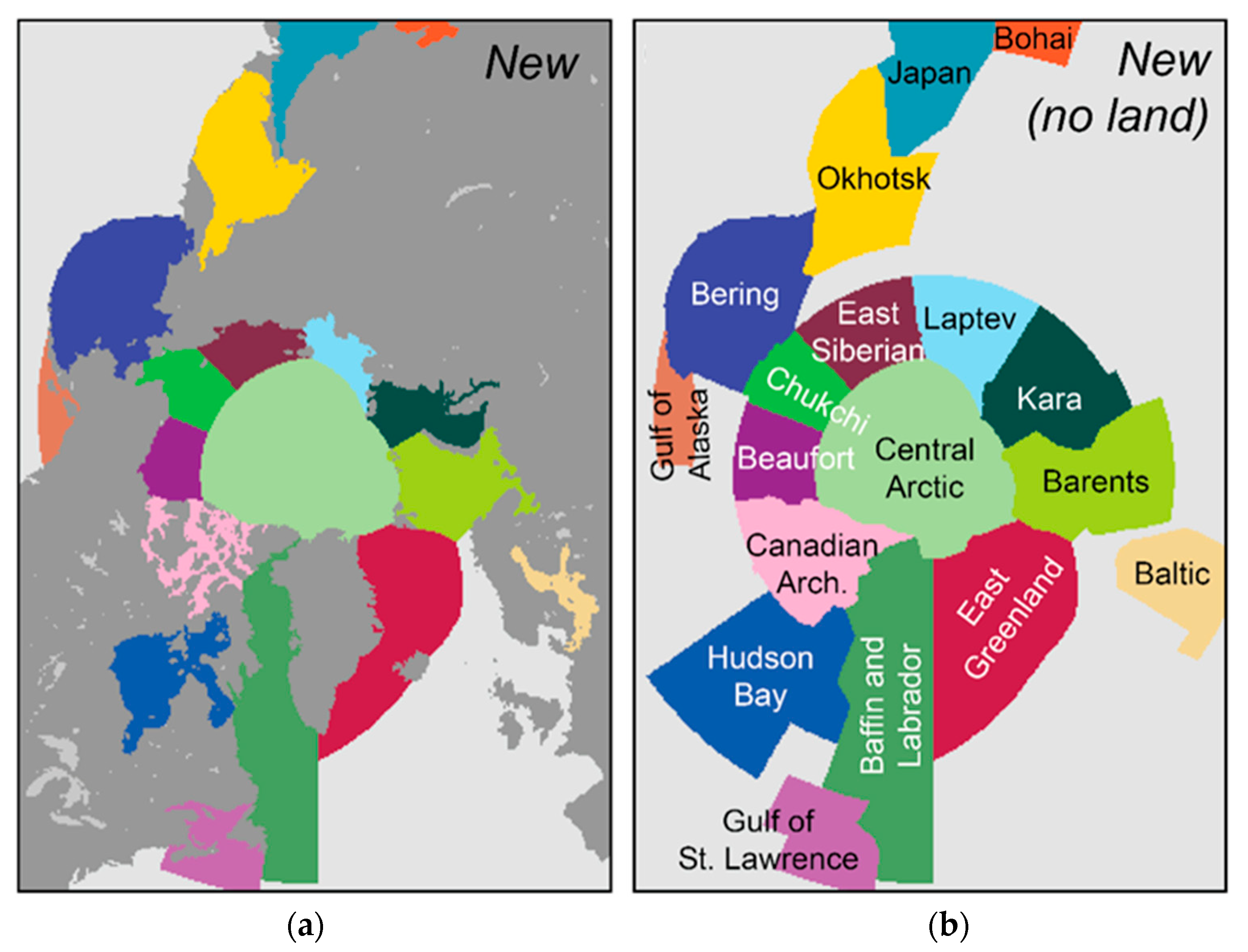
2.3. Subregions of the Arctic

In addition to predicting sea ice extent for the entire Arctic region, we also conducted simulations for various subregions. This research focuses on the following subregions in Figure 1: the seas of Okhotsk and Japan, the Bering Sea, Hudson Bay, Baffin Bay, the Greenland Sea, Kara and Barents Sea, Canadian Archipelago, Gulf of St. Lawrence, and the remaining areas of the Arctic Ocean. By analyzing sea ice extent in these specific subregions, we can gain insights into the localized variations and trends within the Arctic.

3. Results

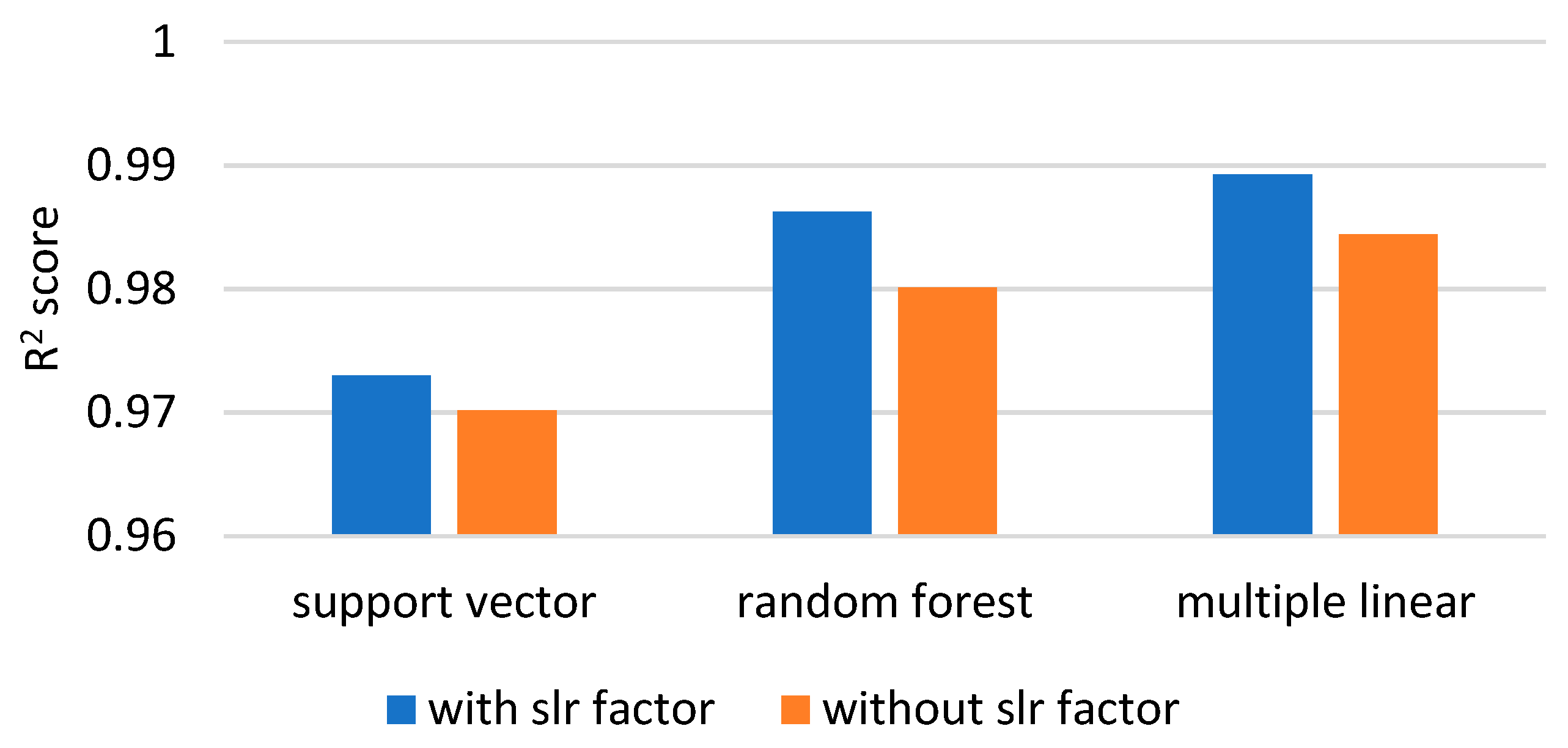
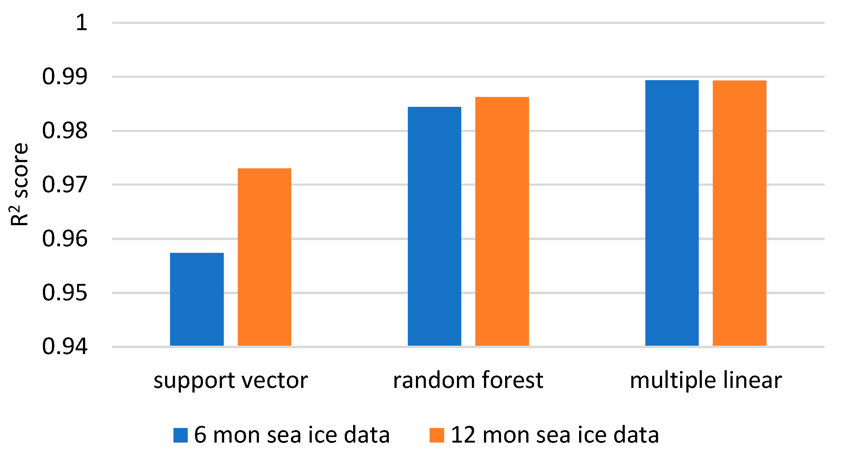
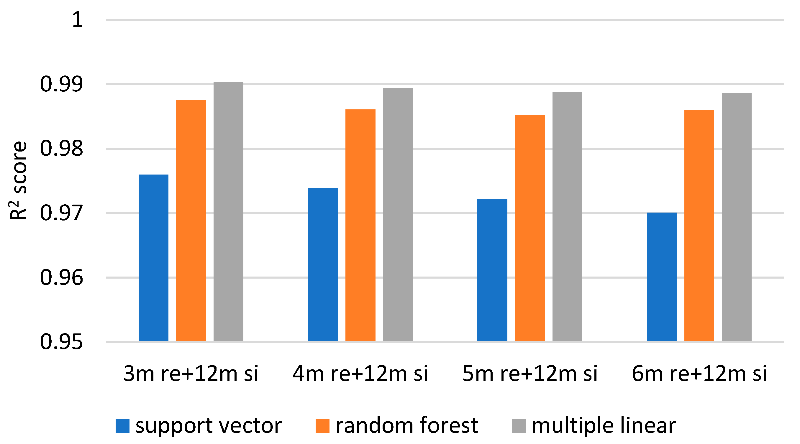
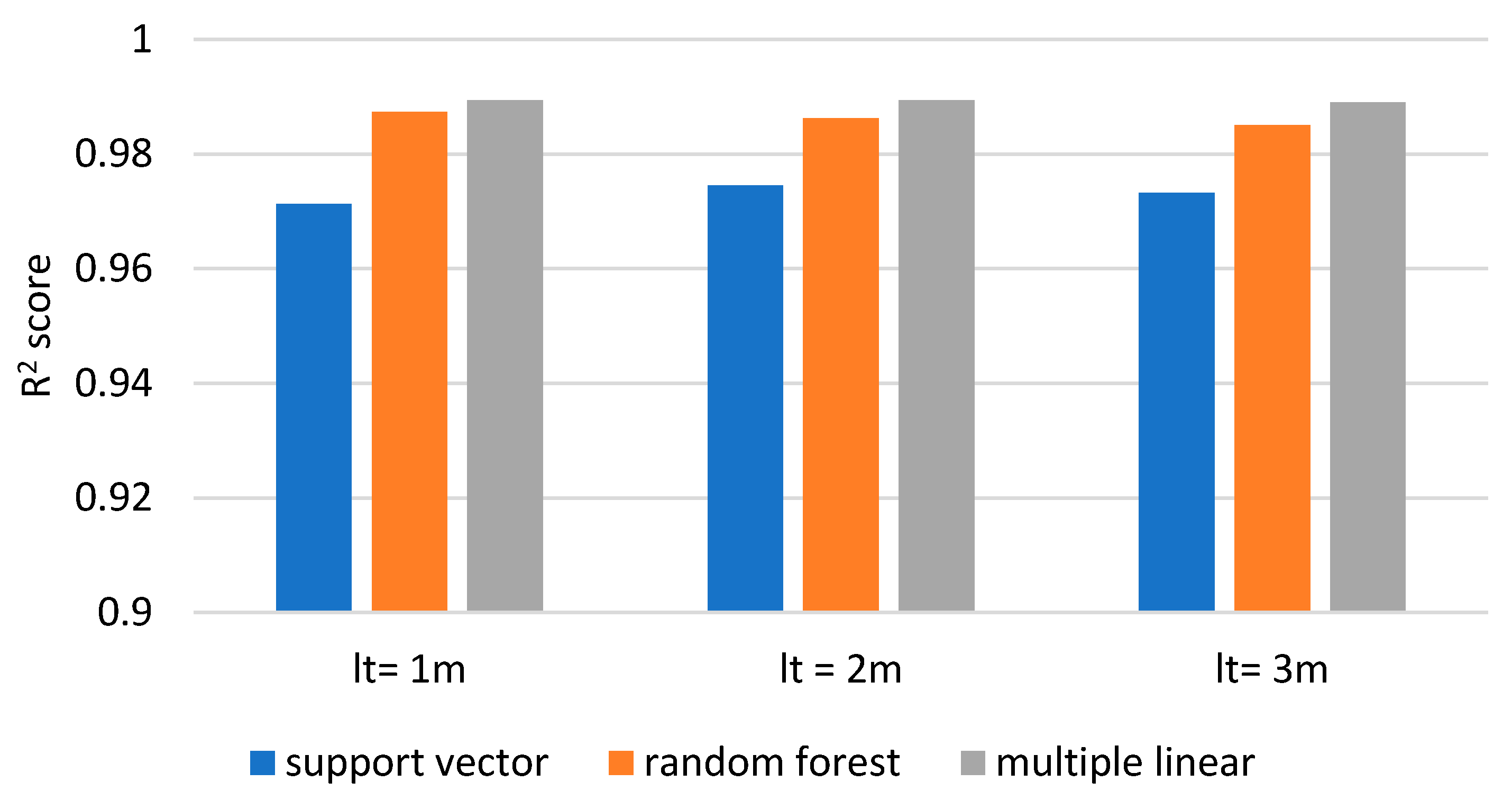
3.1. Whole-Arctic Experiments

Figure 2 presents a comparison of the R2 scores for a sea ice concentration simulation using the support vector model, random forest model, and multiple linear models with and without the simple linear regression factor. It is evident that the inclusion of the simple linear regression factor led to improved results. This can be attributed to the nature of the linear regression factor, which represents part of the seasonal variation in sea ice. By incorporating this factor, the R2 scores for the three models increased by 0.29%, 0.62%, and 0.49%, respectively. These increases were significant given the initially high values of the R2 scores. As a result, the simple linear regression factor was considered an important component in further experiments.
Additionally, among the three machine learning methods, the multiple linear regression method demonstrated a noticeably better performance compared with the other two. Particularly when the simple linear regression factor was included, the R2 score reached nearly 99%. Nevertheless, the support vector regression and random forest regression models still exhibited strong performances, with R2 scores of 97.3% and 98.6%, respectively. The superior performance of multiple linear regression, compared to other methods, typically suggests that the underlying relationships between the sea ice extent and the predictor variables incorporate climate variables and previous sea ice extents. This also implies that the simulation of sea ice extent through a simple linear model is principally linear in nature.
Furthermore, Figure 3 illustrates the impact of the length of the sea ice data time period on the R2 score, while controlling all other factors. Generally, using 12-month sea ice data yields superior results compared with using 6-month data. This is particularly true for the support vector model, which saw a 1.64% increase in R2 score when the time period was extended to 12 months.
It is not surprising to observe that using 12-month sea ice data resulted in better simulations, as it included data from the same month or season of the previous year. This inclusion enhanced the relationship between the factors and the simulation object, leading to improved model performance.
Next, the length of past sea ice extent (SIE) data was set to 12 months. Figure 4 demonstrates that shorter time lengths of the reanalysis climate data correspond to higher R2 scores in the simulation. This contrasts with the findings in Figure 3, where longer past SIE data was shown to improve performance. The disparity in the results may be attributed to the characteristics of the atmosphere, ocean, and sea ice, which can vary and influence the relationship between the factors and the simulation.
The atmosphere, characterized by its low heat capacity, is highly responsive to changes in energy inputs, such as variations in solar radiation or greenhouse gas concentrations [20]. Consequently, atmospheric conditions can exhibit rapid variations. However, this quick response time also implies a short memory for the atmosphere: it quickly adjusts to changes in energy input. On the other hand, the ocean, with its higher heat capacity, responds more slowly to energy input changes. This enables the ocean to store a larger amount of heat over longer periods compared with the atmosphere [21]. As a result, the ocean exhibits a longer memory, retaining the influence of past conditions and impacting long-term climate trends [22]. Sea ice, being a component of the ocean system, exhibits characteristics of both the atmosphere and the ocean. It shares similarities with the atmosphere in terms of its ability to respond relatively quickly to changes in atmospheric conditions, such as air temperature and wind [23]. Like the ocean, sea ice also has a longer memory due to its interaction with the underlying ocean, which allows it to retain the influence of past conditions and impact long-term climate trends [24]. The interaction between sea ice and the underlying ocean introduces a longer memory characteristic. The ocean, with its higher heat capacity, responds more slowly to changes in energy input. This means that the ocean can store a larger amount of heat over longer periods compared with the atmosphere. Consequently, the presence of sea ice can have a feedback effect on the ocean, affecting its circulation patterns, heat distribution, and nutrient cycles. These interactions can persist over time and influence long-lasting ocean and climate patterns.
In addition to these factors, the leading time of the climate variables may also influence the simulation results. Figure 5 presents the outcomes obtained by varying the leading time in the three models.
According to Figure 5, it is evident that shorter leading times tended to yield better results, although this variation is not as pronounced in the support vector regression method. This outcome can be attributed to the shorter memory of the atmosphere, which indicates that climate variables have a rapid influence on the representation of sea ice extent. In other words, the atmospheric conditions and climate variables play a crucial role in shaping the behavior of sea ice extent, and their impact is more immediate and significant in the short term.
As the leading time decreased, the prediction models had access to more up-to-date and relevant climate variables, allowing them to capture the current atmospheric conditions and their effects on sea ice extent more accurately. This led to improved prediction performance, as the models could adapt to the rapidly changing atmospheric conditions that directly influence the sea ice extent. For the entire Arctic region, the optimal combination for the multiple linear regression model involved a leading time of 1 month, a time length of the climate data of 3 months, and a past SIE data length of 12 months. With this configuration, the R2 score for the prediction reached 99.1%.
It is important to note that while shorter leading times generally yielded better results, the support vector regression method exhibited less variability in performance across different leading times. This may be due to the inherent characteristics of the support vector regression algorithm, which can effectively extract patterns and relationships from the available data, even when considering longer leading times.

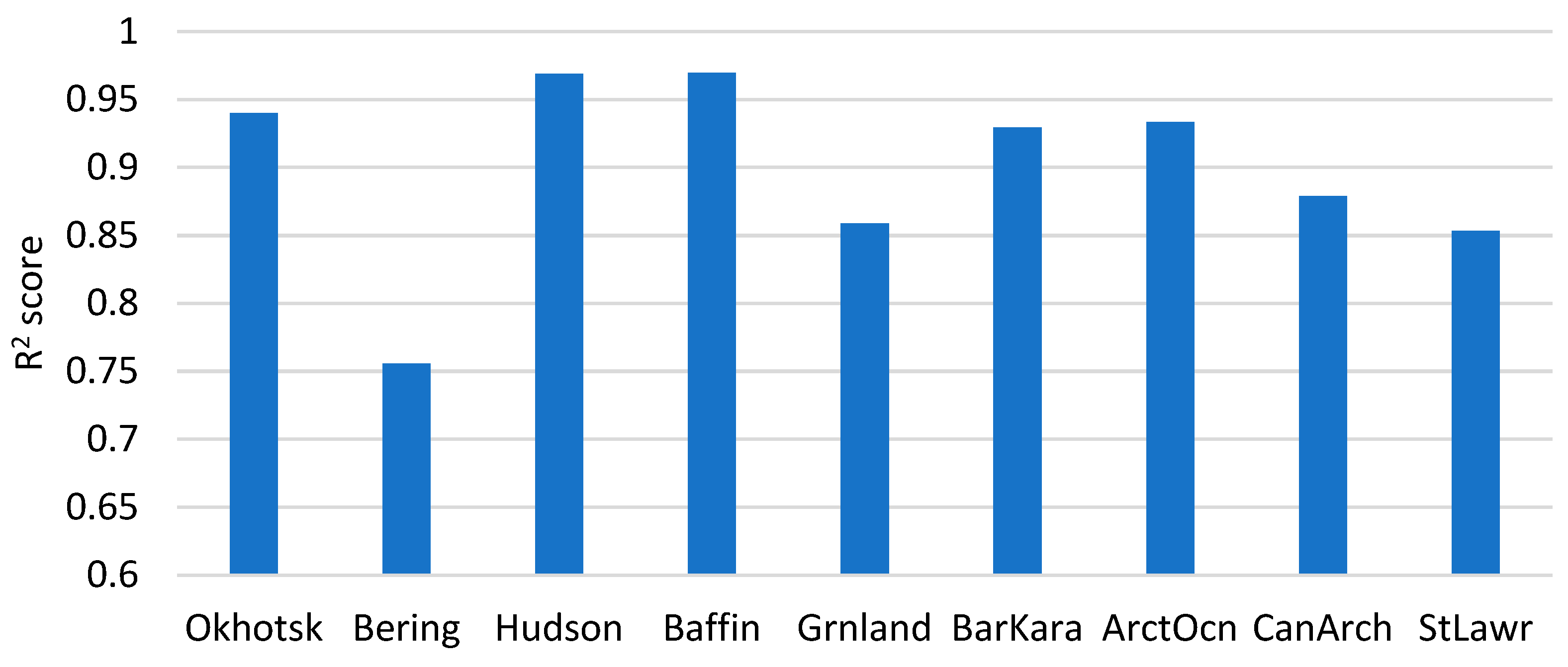
3.2. Arctic Subregion Experiments

In the subregion research, we maintained the combination that yielded the best results in the total-Arctic simulation. Figure 6 presents the varying performances of the different subregions.
The results indicate that the central Arctic region generally exhibited good performance with the multiple linear regression method. This can be attributed to the relatively small variation in sea ice throughout the year in this region. The stability of sea ice in the central Arctic allowed for more accurate predictions using the multiple linear regression approach. The limited fluctuations in sea ice extent made it easier to establish meaningful relationships between predictor variables and sea ice extent.
On the other hand, the Bering Sea region showed the poorest prediction results, highlighting the challenges posed by its significant sea ice variability. The Bering Sea experienced substantial fluctuations in sea ice extent due to freezing and melting processes, which have a profound impact on various physical and biological parameters of the sea. The prediction accuracy in this region was adversely affected by its dependence on multiple factors, such as air temperature, wind patterns, and ocean currents.
In our analysis, we utilized fixed past sea ice extent and climate data to simulate sea ice extent in a specific location. However, we did not consider the influence of surrounding regions and climate variabilities, which is a notable limitation. The omission of these factors can result in larger errors, particularly in regions characterized by substantial sea ice variability and rapidly changing and harsh weather conditions. By neglecting the interconnectedness between different regions and climate fluctuations, our predictions may not fully capture the intricate dynamics that affect sea ice extent. Future research should aim to incorporate a more comprehensive and holistic approach that considers the broader climate context and the interactions between different regions in order to improve the accuracy of sea ice extent predictions.
Additionally, it is interesting to note that Hudson Bay and Baffin Bay exhibited the highest R2 scores for sea ice extent prediction using machine learning methods. These regions, characterized by their high predictability, offer valuable insights into the factors influencing ice cover. One of the contributing factors to the higher R2 scores in Hudson Bay and Baffin Bay is their relatively reduced susceptibility to the influence of complex ocean currents and topography, especially when compared with regions such as the Bering Sea. Unlike the Bering Sea, which experiences intricate interactions between oceanic currents and varying topographic features, Hudson Bay and Baffin Bay are relatively enclosed bodies of water. This relative isolation from global oceanic currents simplifies the predictability of ice cover in these regions. Furthermore, the presence of predictable seasonal patterns closely tied to shifts in temperature also contribute to the higher R2 scores observed in Hudson Bay and Baffin Bay. The annual cycle of ice growth and melt in these regions follows a more regular pattern due to the predictable seasonal shifts in temperature. These temperature variations play a significant role in determining the freeze and thaw patterns of the ice cover. The consistent and predictable nature of these temperature shifts makes the annual cycle of ice growth and melt more predictable, particularly when captured by machine learning models. Despite experiencing significant variation in ice cover, the freeze and thaw patterns in Hudson Bay and Baffin Bay exhibited a strong correlation with the predictable seasonal shifts in temperature. This relationship enhanced the predictability of the ice conditions, allowing machine learning models to capture and accurately predict the behavior of ice extent in these regions. In contrast, the Bering Sea is well-known for its unpredictable and severe storms, which can rapidly alter sea ice conditions. The Bering Sea is prone to sudden and extreme weather events that can cause significant fluctuations in ice cover. These unpredictable and severe storms introduced a high degree of variability, making it more challenging to accurately predict sea ice extent in this region using machine learning methods. While severe weather conditions can also occur in Hudson Bay and Baffin Bay, such events are generally less frequent compared with those in the Bering Sea. As a result, the ice conditions in Hudson Bay and Baffin Bay tended to be more stable and predictable. This increased stability and predictability contributed to the higher R2 scores observed in these regions.
In summary, the higher R2 scores in Hudson Bay and Baffin Bay can be attributed to the reduced influence of complex ocean currents and topography, as well as the presence of predictable seasonal patterns closely tied to shifts in temperature. In contrast, the Bering Sea’s susceptibility to unpredictable and severe storms leads to less stable and less predictable ice conditions, resulting in lower R2 scores in that region.

4. Conclusions

In this research, we explored the potential of using machine learning methodologies for the prediction of sea ice extent in the Arctic region. This is of profound importance due to the rapid decline of Arctic Sea ice in recent years, a key indicator of global warming that can affect various feedback processes in the Arctic ecosystem. Therefore, accurate and timely predictions of sea ice extent and thickness can significantly contribute to the efficacy of climate modeling and subsequent climate predictions. The addition of a simple linear-regression-simulated sea ice extent factor improved the model’s performance by incorporating seasonal variations. Additionally, a shorter leading time and time length of climate variables were found to enhance the modeling results. Conversely, a longer time length of past sea ice extent data positively influenced the R2 score, likely due to the longer memory of the ocean and sea ice compared with the atmosphere.
For the whole Arctic region, the optimal combination was a multiple linear regression model with a leading time of 1 month, a time length of climate data of 3 months, and a time length of past sea ice extent data of 12 months. This combination yielded an impressive R2 score of 99.1% for sea ice extent prediction.
Regarding subregions, the same combination that performed well in the total-Arctic simulation was used. The central Arctic region, characterized by minimal sea ice variation throughout the year, showed good simulation results with the multiple linear regression model. On the other hand, the Bering Sea region exhibited relatively poorer performance, potentially due to the limitations of the experimental setup. The influence of sudden weather changes and significant seasonal variability in the Bering Sea region could have also contributed to the lower R2 score. To improve accuracy, expanding the spatial range of the subregional factor data specific to each subregion could be considered. Furthermore, regions such as Hudson Bay and Baffin Bay, which experience less influence from sudden weather changes and have predictable seasonal patterns, demonstrated very high R2 scores in the simulation.
Despite the promising results, it is important to note the limitations of the current study. Machine learning methods, particularly multiple linear regression, proved effective in predicting sea ice extent in the Arctic region, but performance varied considerably across different subregions due to differences in local weather patterns and sea ice conditions. This indicates that the model may not account for all complexities and regional specifics of sea ice dynamics. Additionally, the sudden and significant seasonal changes in regions such as the Bering Sea underline the need for models that can handle rapid environmental shifts.
In the future, the potential applications of this work are expansive. Improved sea ice predictions can inform policy decisions, climate mitigation strategies, and marine navigation safety measures. Moreover, as our understanding and ability to model Arctic Sea ice dynamics continues to grow, these predictions can provide critical insights into global climate patterns and their links to sea ice extent. Future research should therefore focus on refining and enhancing the model’s performance in more challenging regions, incorporating more dynamic factors to increase accuracy, and extending its application to other climate prediction tasks.

Author Contributions

Conceptualization, S.C. and Y.C.W.; methodology, S.C.; software, H.F.; validation, H.F. and Y.C.W.; formal analysis, K.L.; investigation, K.L. and Y.C.W.; resources, Y.H.; data curation, Y.C.W.; writing—original draft preparation, S.C.; writing—review and editing, H.F.; visualization, Y.C.W.; supervision, Y.H.; project administration, Y.H. All authors have read and agreed to the published version of the manuscript.

Funding

This research received no external funding.

Institutional Review Board Statement

Not applicable.

Informed Consent Statement

Not applicable.

Data Availability Statement

The data that support the findings of this study are available from the corresponding author upon reasonable request.

Conflicts of Interest

The authors declare no conflict of interest.

References

  1. Serreze, M.C.; Stroeve, J. Arctic sea ice trends, variability and implications for seasonal ice forecasting. Philos. Trans. R. Soc. A 2015, 373, 20140159. [Google Scholar] [CrossRef] [PubMed] [Green Version]
  2. Cohen, J.; Screen, J.A.; Furtado, J.C.; Barlow, M.; Whittleston, D.; Coumou, D.; Francis, J.; Dethloff, K.; Entekhabi, D.; Overland, J.; et al. Recent Arctic amplification and extreme mid-latitude weather. Nat. Geosci. 2014, 7, 627–637. [Google Scholar] [CrossRef] [Green Version]
  3. Post, E.; Alley, R.B.; Christensen, T.R.; Macias-Fauria, M.; Forbes, B.C.; Gooseff, M.N.; Iler, A.; Kerby, J.T.; Laidre, K.L.; Mann, M.E.; et al. The polar regions in a 2 °C warmer world. Sci. Adv. 2019, 5, eaaw9883. [Google Scholar] [CrossRef] [PubMed] [Green Version]
  4. Huntington, H.P.; Loring, P.A.; Gannon, G.; Gearheard, S.F.; Gerlach, S.C.; Hamilton, L.C. Staying in place during times of change in Arctic Alaska: The implications of attachment, alternatives, and buffering. Reg. Environ. Chang. 2017, 17, 897–906. [Google Scholar] [CrossRef] [Green Version]
  5. Laidre, K.L.; Stern, H.; Kovacs, K.M.; Lowry, L.; Moore, S.E.; Regehr, E.V.; Ferguson, S.H.; Wiig, Ø.; Boveng, P.; Angliss, R.P.; et al. Arctic marine mammal population status, sea ice habitat loss, and conservation recommendations for the 21st century. Conserv. Biol. 2020, 34, 630–643. [Google Scholar] [CrossRef] [PubMed] [Green Version]
  6. Screen, J.A.; Simmonds, I. The central role of diminishing sea ice in recent Arctic temperature amplification. Nature 2010, 464, 1334–1337. [Google Scholar] [CrossRef] [PubMed] [Green Version]
  7. Pistone, K.; Eisenman, I.; Ramanathan, V. Radiative Heating of an Ice-Free Arctic Ocean. Geophys. Res. Lett. 2019, 46, 7474–7480. [Google Scholar] [CrossRef]
  8. Carrieres, T.; Buehner, M.; Lemieux, J.-F.; Pedersen, L.T. Sea Ice Analysis and Forecasting: Towards an Increased Reliance on Automated Prediction Systems; Cambridge University Press: Cambridge, UK, 2017. [Google Scholar]
  9. Notz, D.; Stroeve, J. Observed Arctic sea-ice loss directly follows anthropogenic CO2 emission. Science 2016, 354, 747–750. [Google Scholar] [CrossRef] [PubMed] [Green Version]
  10. Stroeve, J.; Notz, D.; Gerland, S. Arctic sea ice in decline: Faster than forecast. Geophys. Res. Lett. 2018, 45, 9169–9176. [Google Scholar] [CrossRef]
  11. Intergovernmental Panel on Climate Change (IPCC). Evaluation of Climate Models. In Climate Change 2013: The Physical Science Basis; Flato, G., Marotzke, J., Abiodun, B., Braconnot, P., Chou, S.C., Collins, W., Cox, P., Driouech, F., Emori, S., Eyring, V., Eds.; Cambridge University Press: Cambridge, UK; New York, NY, USA, 2013. [Google Scholar]
  12. Stroeve, J.C.; Kattsov, V.; Barrett, A.; Serreze, M.; Pavlova, T.; Holland, M.; Meier, W.N. Trends in Arctic sea ice extent from CMIP5, CMIP3 and observations. Geophys. Res. Lett. 2012, 39, L16502. [Google Scholar] [CrossRef] [Green Version]
  13. Webster, M.; Gerland, S.; Holland, M.; Hunke, E.; Kwok, R.; Lecomte, O.; Massom, R.; Perovich, D.; Sturm, M. Snow in the changing sea-ice systems. Nat. Clim. Chang. 2018, 8, 946–953. [Google Scholar] [CrossRef]
  14. Persson, P.O.G. Onset and end of the summer melt season over sea ice: Thermal structure and surface energy perspective from SHEBA. Clim. Dyn. 2012, 39, 1349–1371. [Google Scholar] [CrossRef]
  15. Carrassi, A.; Bocquet, M.; Bertino, L.; Evensen, G. Data Assimilation in the Geosciences: An Overview of Methods, Issues, and Perspectives. WIREs Clim. Chang. 2018, 9, e535. [Google Scholar] [CrossRef] [Green Version]
  16. Overland, J.E.; Wang, M. Large-scale atmospheric circulation changes are associated with the recent loss of Arctic sea ice. Tellus A 2010, 62, 1–9. [Google Scholar] [CrossRef] [Green Version]
  17. Andreas, E.L.; Cash, B.A. Convective Heat Transfer over Wavy Surfaces. J. Fluid Mech. 1999, 389, 101–139. [Google Scholar]
  18. Peixoto, J.P.; Oort, A.H. Physics of Climate, 1st ed.; American Institute of Physics: New York, NY, USA, 1992. [Google Scholar]
  19. Vallis, G.K. Atmospheric and Oceanic Fluid Dynamics: Fundamentals and Large-Scale Circulation, 2nd ed.; Cambridge University Press: Cambridge, UK, 2017. [Google Scholar]
  20. Frankignoul, C.; Czaja, A.; L’Heveder, B. Air-Sea Feedback in the North Atlantic and Surface Boundary Conditions for Ocean Models. J. Clim. 1997, 10, 2310–2324. [Google Scholar] [CrossRef]
  21. Maykut, G.A. The surface heat and mass balance. In The Geophysics of Sea Ice; Springer: Berlin/Heidelberg, Germany, 1986; pp. 395–463. [Google Scholar]
  22. Steele, M.; Morley, R.; Ermold, W. PHC: A Global Ocean Hydrography with a High-Quality Arctic Ocean. J. Clim. 2001, 14, 2079–2087. [Google Scholar] [CrossRef]
  23. Hakkinen, S.; Proshutinsky, A.; Ashik, I. Sea ice drift in the Arctic since the 1950s. Geophys. Res. Lett. 2008, 35, L19704. [Google Scholar] [CrossRef] [Green Version]
  24. Reid, T.G.R.; Tarantino, P.M. Predicting Arctic sea ice concentration using a support vector machine. Cryosphere 2022, 16, 137–152. [Google Scholar]
Figure 1. Study area: (a) The Arctic, (b) The Subregion of the Arctic. National Snow and Ice Data Center. (2019). 2019 Arctic Sea Ice Minimum Ties for Second Lowest. NSIDC Special Report-25.
Atmosphere 14 01023 g001
Figure 2. R2 score of different models including or excluding the simple linear regression factor of monthly sea ice.
Atmosphere 14 01023 g002
Figure 3. R2 score of different models with different time lengths of past SIE data.
Atmosphere 14 01023 g003
Figure 4. R2 score of different models with different time lengths of reanalysis climate data.
Atmosphere 14 01023 g004
Figure 5. R2 score of different models with different leading times of reanalysis climate data.
Atmosphere 14 01023 g005
Figure 6. R2 score of the subregions with multiple linear regression model; the leading time equals 1 month, and the time length of the climate data and the past SIE data are, respectively, 3 months and 12 months.
Atmosphere 14 01023 g006
Table 1. The setting of the experiments for predicting sea ice extent in the Arctic.
StageTested ParameterTested Value
1Simple linear regression SIEAdd this factor or not
2Machine learning methodsSupport vector regression, random forecast regression, and multiple linear regression methods
3Reanalysis variables3, 4, 5, 6 months of the length of these variables
4Past SIE6 or 12 months of past SIE
5Leading time1, 2, or 3 months of leading time
6RegionTotal Arctic or subregions
Disclaimer/Publisher’s Note: The statements, opinions and data contained in all publications are solely those of the individual author(s) and contributor(s) and not of MDPI and/or the editor(s). MDPI and/or the editor(s) disclaim responsibility for any injury to people or property resulting from any ideas, methods, instructions or products referred to in the content.

