The Influence of Wind-Induced Response in Urban Trees on the Surrounding Flow Field

Abstract

In recent years, cities have experienced frequent climate changes and deteriorating wind environments. Urban vegetation has become an important measure to improve local microclimates with its flexible configuration. Leaves and branches also reorient with the direction of wind, affecting the airflow through the tree. However, trees are usually considered as stationary porous media areas and are not influenced by wind speed in existing numerical simulation studies. Therefore, by considering the response of a tree under natural wind, this study established a fitted relationship between porosity and wind speed by measuring the porosity of trees at different wind speeds in the field. A numerical model of the wind response of the tree was developed, and the tree drag coefficient was changed using the additional source term method to verify the feasibility of the model by measuring the wind environment behind the tree. To understand the effect of the wind-induced response on the surrounding flow field and its variation pattern, the surrounding flow fields of stationary tree (T-S) and wind-induced tree (T-D) at different wind speeds were compared and analyzed. The effect of porosity and height-to-width ratio under the wind-induced response of trees on the wind environment were quantified. It was found that at different wind speeds, as the wind speed increases, the tree porosity gradually increases and the drag coefficient decreases accordingly. The effective shading distance after wind response was 2.4H, which was 0.3H less compared to vertically fixed trees. The minimum wind speed increased linearly with plant porosity, and the minimum wind speed occurrence location and wind speed recovery distance were linearly and negatively correlated with tree height-to-width ratio. Therefore, the flow field around the tree was simulated to provide references for guiding tree planting and mitigating urban wind environments.

1. Introduction

In recent years, global warming has intensified, and the urban climate is changing frequently [1], with the microclimate of urban habitats undergoing profound changes. At the same time, as urbanization progresses, the increasing height and density of buildings has led to a ‘complication’ of air flow [2]. The urban wind environment has attracted the attention of academics. The wind environment is the wind field formed by outdoor natural wind, which is influenced by urban topography or natural topography [3]. A suitable wind environment can effectively improve microclimate comfort, alleviate the heat island effect and disperse air pollutants [4,5,6], which is directly related to the level of the human living environment and the health of residents. Based on existing urban planning, the question of how to improve the local microclimate and people’s quality of life through environmental design needs to be addressed. As one of the fundamental elements of the city, urban green space has an important influence on microclimate with its flexible configuration [7] and is an important initiative to improve the wind environment. Therefore, it is necessary to have a comprehensive understanding of the changing laws of the flow field around trees to guide urban tree planting, which is of great practical significance for building a comfortable and healthy urban wind environment, creating a liveable urban ecological environment and achieving sustainable urban development.

It has been demonstrated that vegetation, especially trees in urban areas, has a favorable effect on the local wind environment [8,9]. On the one hand, trees reduce the wind speed behind them in urban areas by hindering the high-speed flow of incoming wind [10], changing the fluidity of the adjacent areas near the ground [11] and improving the comfort and health of the wind environment. On the other hand, due to the obstructive effect of the vegetation on the incoming wind, a lateral diversion is created, and part of the airflow is squeezed to the outside of the canopy, creating an acceleration zone on both sides of the canopy. Currently, scholars classify the wind field around vegetation into an upwind light deceleration zone, an acceleration zone on both sides and a downwind deceleration zone based on the trend of wind speed [12,13]. In these areas, wind speed in the downwind zone directly affects wind protection distance and effectiveness [14]. It receives extensive research attention because of significant airflow velocity variation [15,16,17]. The overall airflow variation in the downwind zone of a single tree is usually represented by the airflow variation in the central axis of the tree, based on which studies have developed airflow field models around single plants [13,18] to quantify the effect of tree characteristics on the flow field model parameters.

Under the action of natural winds, trees can experience significant top displacement, crown contraction and trunk bending due to the flexibility and permeability of their branches and leaves. Cao et al. [19] and Zhang et al. [20] analyzed the wind-induced response of trees with different characteristics and deformation capacities, and they analyzed the relationships between changes in tree characteristics and wind speed, such as crown displacement, windward area and porosity. Rudnicki et al. [21] noted that the classical resistance equation for a porous, flexible canopy is problematic because the windward area of the canopy decreases as wind speed increases and branch streamlining increases. The wind-induced response of trees leads to a change in their own characteristics and has an effect on the surrounding flow field, especially at high wind speeds, where leaves and branches can reorient themselves along the wind direction, affecting the flow path and the resulting drag coefficient [22,23], leading to a change in the intensity and extent of the tree’s influence on the surrounding flow field. Therefore, the study of the wind environment around trees is premised on the consideration of changes in the wind-induced response of trees. He and Li [24] studied the wind response of trees through wind tunnel tests and further investigated the effect of trees on the wind environment around low buildings after wind response occurred. Li [25] used small saplings of bean-petaled boxwood as a test model to investigate the differences in wind response of trees and the effect on the wind environment behind the trees under different canopy morphology, arrangement and porosity conditions through wind tunnel tests.

The main methods used to study the flow field around trees include in situ measurements, wind tunnel tests and numerical simulations. Field measurements can only measure a limited number of velocity points due to the limitations of the conditions. Wind tunnel tests rely on the use of scaled-down models for the prediction of flow fields, and although the model trees adequately mimic the appearance and shape of natural trees, the mechanical properties of the trees are not scaled, such as the modulus of elasticity and bending stiffness [26]. Both of these have limitations in reproducing the effects of real trees in cities. In recent years, the turbulent airflow field around trees has been widely simulated using computational fluid dynamics (CFD) technology. Due to the complex morphological structure of trees, previous studies have simplified tree canopies into elliptical, square, rectangular and other geometries and equated them to porous media to analyze the effect of trees on the flow field [27,28,29]. It has been shown that the porosity is not constant during the flow of air [30,31,32]. Li et al. [33] set up drag coefficients at different wind speeds based on wind tunnel tests to further investigate the flow field characteristics of tree drag coefficients that change with wind speed. At present, most of the numerical simulation studies on tree flow fields have always considered trees as a vertically fixed porous media region, and they have only considered that porosity varies with tree species, neglecting the dynamic changes in porosity due to the tree wind-induced response.

Urban trees, with flexible arrangements, are an important initiative to improve the urban wind environment. Therefore, this research considers the response of trees to wind speed and reproduces the real change state of trees under natural wind. The computational fluid dynamics (CFD) technique is used to study the flow field around the tree. The response of trees to wind speed is considered, and a numerical model of the wind-induced response of trees is established by measuring the porosity of a tree at different wind speeds in the field. The fitting relationship between porosity and wind speed is established, while the drag coefficient of trees under different degrees of stress is changed by the additional source method. The model is validated by measuring the wind environment behind the tree. The wind response characteristics of the tree are investigated and analyzed, and the surrounding flow fields of vertically fixed tree (T-S) and wind-responsive tree (T-D) at different wind speeds are compared and analyzed to quantify the effect of wind response-induced changes in porosity and aspect ratio on the wind environment and to establish the fitted relationships with minimum wind speed, minimum wind distance and wind recovery distance.

2. Research Method

2.1. Governing Equation

It is assumed that the air in the basin is an incompressible ideal gas. The governing equations of momentum are shown in Equation (1). The k-ε turbulence closure model has been used in most previous studies of plant flow fields and windbreaks [34,35], and they proved to be in some agreement with experimental results. Therefore, the standard k-ε model was used in this study.

The governing equations of turbulence and dissipation rate are shown in Equations (1)–(3):

$$u_j\frac{\partial u_i}{\partial x_j}=-\frac{1}{\rho }\frac{\partial p}{\partial x_i}+\frac{\partial }{\partial x_j}\left(v_e\frac{\partial u_i}{\partial x_j}\right)+S_i$$

(1)

$$u_j\frac{\partial k}{\partial x_j}=\frac{\partial }{\partial x_i}\left(\frac{v_t}{{\sigma }_k}\frac{\partial k}{{\partial x}_i}\right)+v_t\left(\frac{{\partial u}_i}{{\partial x}_j}+\frac{{\partial u}_j}{{\partial x}_i}\right)\frac{{\partial u}_i}{{\partial x}_j}-\epsilon +S_k$$

(2)

$$u_j\frac{\partial \epsilon }{{\partial x}_j}=\frac{\partial }{{\partial x}_i}\left(\frac{v_t}{{\sigma }_{\epsilon }}\frac{\partial \epsilon }{{\partial x}_i}\right)+C_{\epsilon 1}\frac{\epsilon }{k}{v}_t\left(\frac{{\partial u}_i}{{\partial x}_j}+\frac{{\partial u}_j}{{\partial x}_i}\right)\frac{{\partial u}_i}{{\partial x}_j}-C_{\epsilon 2}\frac{{\epsilon }^2}{k}+S_{\epsilon }$$

(3)

where p (Pa) is the air pressure; ρ (kg/m³) is the density of the airflow; ν_e (-) is the viscosity coefficient of the airflow; ν_t (-) is the turbulent viscosity coefficient; and C_ε1 (-) and C_ε2 (-) are dimensionless constants, which are 1.42 and 1.92, respectively. S_i (K·gm⁻²·s⁻²), S_k (kg·m⁻¹·s⁻³) and S_ε (kg·m⁻¹·s⁻⁴) are the momentum source term, turbulent kinetic energy term and turbulent dissipation rate source term, respectively.

According to the vegetation modeling concepts of Green [36] and Liu et al. [37], the resistance of the tree canopy to airflow and the increase in turbulence intensity caused by the trees were considered. The loss of velocity and pressure is described by adding source terms to the momentum equation, turbulent kinetic energy equation and turbulent dissipation rate equation in the crown, which shows the porous medium characteristics of the crown. The momentum source term, turbulent kinetic energy term and turbulent dissipation rate source term are shown in Equations (4)–(6), respectively. It is used to express the change in airflow through the leaves and branches of plants. Because the Reynolds of airflow is too large, the viscous drag coefficient can be ignored compared with its inertial drag coefficient.

$$S_i=-\frac{1}{2}\rho C_d|u{|u}_i$$

(4)

$$S_k={\stackrel{-}{u}}_i{S}_i-4C_d|{\stackrel{-}{u}}_i|k$$

(5)

$$S_{\epsilon }=\frac{\epsilon }{k}[C_{p\epsilon 1}({\stackrel{-}{u}}_i{S}_i)-C_{p\epsilon 2}(4C_d|{\stackrel{-}{u}}_i|)]$$

(6)

where C_d (-) is the canopy’s drag coefficient, u_i (m/s) is the velocity of the airflow in the i direction, ρ (kg/m³) is the density of the airflow, taking 1.225, and C_ρε1 (-) and C_ρε2 (-) are additional source term coefficients. C_ρε1 (-) is 1.8 and C_ρε2 (-) is 1.5; k (m² s⁻²) is the turbulent kinetic energy; and ε (-) is the turbulent kinetic energy dissipation rate. The relational expression between the drag coefficient C_d and porosity VP is as follows [38]:

$$C_d=1.08\left(1-{VP}^{1.8}\right)$$

(7)

The porosity and drag coefficient of trees will change due to tree reconfiguration, which will affect the airflow through the leaf branches of plants through the control equation. The porosity of Ulmus parvifolia Jacq. at different wind speeds was measured and substituted into the simulated model tree to approximate the change in airflow during tree deformation.

The analytical equation for the transient dynamics of the solid part of the trunk under the air load is:

$$F\left(t\right)=M\ddot{u}+C\dot{u}+Ku$$

(8)

where M, C, and K are the mass matrix, damping matrix, and stiffness matrix, respectively; $\ddot{u}$, $\dot{u}$, and u are the acceleration vector, velocity vector, and displacement vector of the node, respectively; and F(t) is the wind load vector.

The fluid–solid coupling problem can be essentially considered as a continuous exchange of energy between the fluid and the solid in a solution region that contains both the solid and the fluid. In numerical simulation, there is a “fluid-structure interface” between the solid solver and the fluid solver, which is actually a transfer procedure that coordinates the data exchange between the two media.

2.2. Modeling

The L-system was first proposed by American theoretical biologist Aristid Lindenmayer and is the most successful method in plant simulation [39]. Its core idea is the parallel rewriting of strings, which can quickly express the topological structure and geometric shape of plants and has fractal characteristics. This method has obvious advantages in simulating plant morphology and is widely used. The branching structure of trees is an important factor in determining the crown form. The branching modes of trees are generally divided into monopodial branching, sympodial branching and false dichotomous branching. Sympodial branching, which has an open crown, is very common in reality.

To clarify the deformation of trees and the surrounding flow field, the tree model is established step by step. The detailed design processes are as follows.

First, the stationary tree model is established, including the main branch solid model and the leaf area porous region. The basic branch model of the synthetic branch tree is established according to the L-system. The small branch and leaf areas are considered as a whole. The porous medium model of the crown is established based on the additional source item, in which the form is simplified into a semiellipsoid to describe the outer contour of the branch. The size of the model tree is from the Ulmus parvifolia Jacq. through field measurements. The tree height is 6.8 m, the trunk height is 1.8 m, and the crown width at the widest point is 9 m. The stationary tree is shown in Figure 1a. The elastic modulus determines the mechanical material properties of branches referred to by Hu [40]. The specific parameters are shown in

Table 1. Mechanical material properties of branches.

	Density (kg m−3)	ET (Pa)	EL (Pa)	μLT	μRL	GLR (Pa)
branch	850	2.0 × 109	0.8 × 103	0.3	0.1	4 × 108

.

The second step is to obtain the deformed branches under controlled wind speed by the fluid–solid coupling method. Deformed trees under the control of wind speed are obtained based on single fluid–solid coupling. Only the unidirectional force of the wind on the tree is calculated, and the reaction force of trees to wind is not considered. The deformed model of branches is obtained in Figure 1b.

In the third step, the deformed leaf area porous model is established based on the additional source method. The porous medium model of the crown is established through the deformed branch. The established method of the deformed crown model is consistent with the first step. The deformed tree is shown in Figure 1c. At this time, the same control wind speed is set up to simulate the flow condition of the surrounding air flow after the tree undergoes deformation under wind speed.

2.3. Grid Division and Boundary Conditions

The calculation domain is illustrated in Figure 2. To ensure the full development of wind turbulence and a reasonable calculation time, the optimum size is set. The calculation domain size is based on a single tree height H. The inflow boundary is set at 5H from the target object boundary, the outflow boundary is set at 15H from the target object boundary, and the height of the entire domain is 5H. The computational domain in this study is established by following the best practice guidelines [41,42].

The meshing software Ansys Mesh 2020R2 is used for generating the gird. The distribution of mesh is shown in Figure 3. Due to the irregular shape of the tree, the inner and outer parts are used. Hexahedra cells are used to mesh the outer part. Because of its high calculation accuracy, iteration error is smaller. The grid with trees inside adopts unstructured grids. To fully calculate the airflow, it is locally encrypted, and the area length × width × height is 15 m × 15 m × 7 m. The external grid is a structured grid. The total number of grids is 2,560,715. The blockage rate was 0.7% (<3%).

The lower atmosphere is an incompressible fluid, and the velocity–inlet boundary is suitable for an incompressible fluid. The inlet type is velocity–inlet in this study. Taking into account the gradient winds that form outdoors as the height from the ground increases, the real airflow variation in the atmospheric boundary layer is modeled using a power function wind profile in this paper, as shown in Equations (9)–(11):

$$u_z=\frac{u*}{K}ln\left(\frac{z}{z_0}\right)$$

(9)

$$k=\frac{3}{2}{\left({uI}_u\right)}^2$$

(10)

$$\epsilon =\frac{C_{\mu }^{\frac{3}{4}}{k}^{\frac{3}{2}}}{l}$$

(11)

where z₀ (m) is the aerodynamic roughness; u* (m/s) is the friction velocity; z (m) is the height; u_z (m/s) is the wind speed at this height; K is the Karman constant of 0.4; k (m²/s²) is the turbulent kinetic energy; I_u is the turbulence intensity; C_μ = 0.09 is a constant; ε is the turbulent kinetic energy dissipation rate; and l is the turbulence integral scale.

The outlet of the calculation model is set to outflow. The bottom boundary is set as a wall with roughness 4 × 10⁻⁵. The canopy is set as an interior.

2.4. Simulation Calculation Method

The control equations were solved using Ansys Fluent 2020R2. A standard k-ε model was used for the turbulence model and standard wall functions were used for the near-wall surfaces. The ideal incompressible gas is chosen as the fluid material, and the default values of material parameters are used. The SIMPLEC method is used to decouple the system of velocity–pressure equations, and the SIMPLEC algorithm has a faster convergence rate of calculation compared with the SIMPLE algorithm. The discrete format uses the second-order upwind. The convergence criterion for the steady-state simulations is the reduction in the residuals to below 10⁻⁶.

2.5. Validation of the Model

In order to verify the simulation grid, the independence of the grid is investigated in this paper. Calculations are performed using 2,560,715, 5,409,121 and 9,796,458 grids, which are shown in Figure 4. Compare the effect of the number of grids on the calculation results. The total number of grids is adjusted by changing the overall number of grids.

The wind speed was set to 10 m/s and the canopy drag coefficient C_d was 0.704. To make the data variation more obvious, a height of 3.4 m (0.5H) was selected for wind speed comparison, which is located at the location where the canopy has the greatest influence. The axial velocity distribution of different grids at height 0.5H is shown in Figure 5. It can be obtained that although the grid keeps increasing, there is almost no difference in the calculated wind velocity, and the maximum relative error is 0.5%, which indicates that the sensitivity of the simulation results to the number of grids is low and the numerical solution is more accurate.

3. Model Validation

3.1. Parameter Acquisition

The research area in this paper is located in Lin’an District, Hangzhou City, along the southeast coast of China. The trees were selected for the following reasons: (1) Trees were selected that had the general appearance of the species and were representative of the majority of trees of the same species. (2) The trees are uniform and lush in growth, with no significant skew. (3) The trees are relatively independent in growth and have little overlap with the surrounding trees to facilitate pixilation.

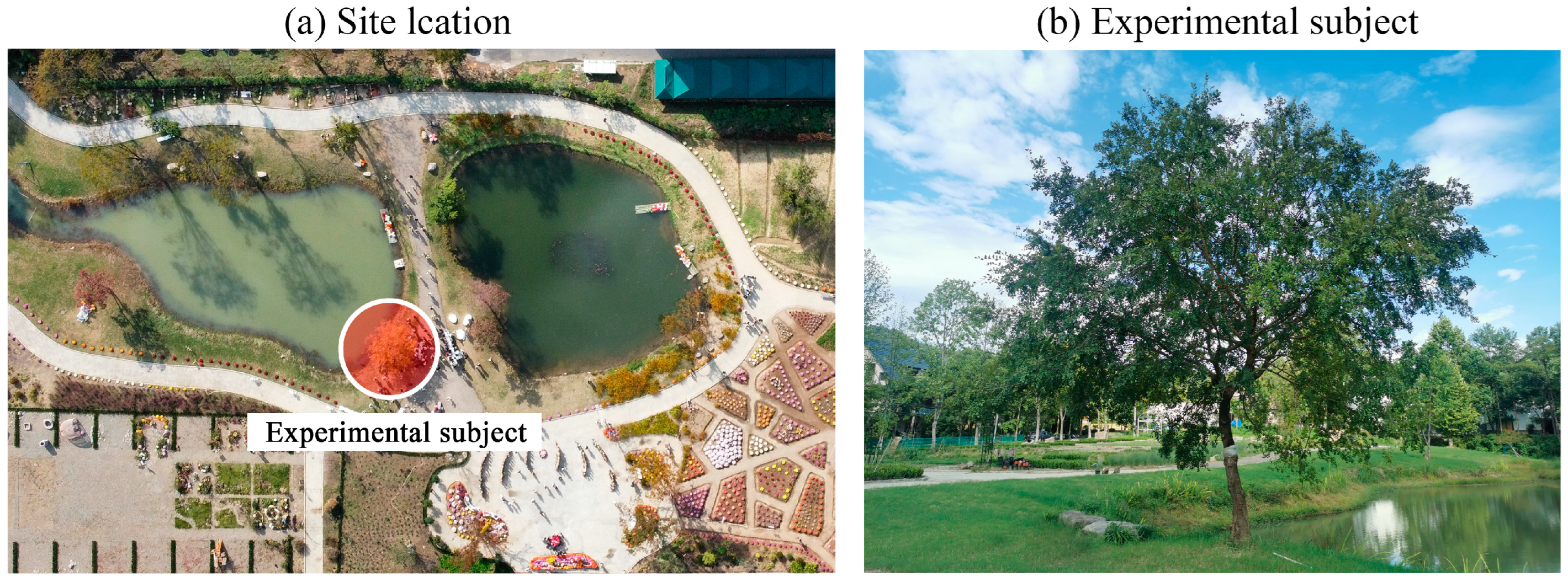
As shown in Figure 6a,b, the selected experimental subject is Ulmus parvifolia Jacq., which is in the education and teaching practice base of Zhejiang Agriculture and Forestry University (30.26° N, 119.73° E). It has good growing conditions. The height of the tree is 6.8 m, the trunk height is 1.8 m, the diameter at breast height is 0.6 m, and the crown width is 9 m. The site is open, with no significant deflection observed. The canopy is in a uniform and luxuriant state of growth.

Kennew [43] demonstrated that the two-dimensional porosity of plants can be measured using digitized photographs, a commonly used and relatively readily available method for characterizing plant structure. Photographs were taken to record the characteristics of the windward and crosswind sides of trees at different wind speeds without disturbing the flow field in front of the trees. A Fuji camera X-T2 with up to 24.1 million pixels was used to take images of the tree canopy, and the photographed trees were pixelated with the aid of Adobe Photoshop CS6 software to accurately calculate the porosity of the trees at different wind speeds.

The porosity was recorded at different wind speeds (2, 4, 6, 8 and 10 m/s), and each wind speed was repeated three times and averaged for different wind speeds. The camera is fixed by a tripod in such a way that it does not affect the wind environment around the tree to ensure that the filming azimuth is consistent at different wind speeds and to record the wind speed and velocity at the time of filming. It is advisable to choose a time of day when the wind speed is high for the measurement. Examples of photographs taken are shown in Figure 7.

As shown in Figure 7, there is a significant contraction of the canopy, with the degree of deformation increasing as the wind speed increases and the windward area decreases. As wind speed increases, the canopy deforms significantly, with branches and leaves on the windward side deforming at a significant angle in the direction of the wind, with branches and leaves concentrated on the leeward side. It is mainly the branches above the second and third levels that are subject to contraction and deformation by wind action, with significant changes occurring due to the softer and more flexible nature of the tree’s smaller branches, while the trunk basically does not bend due to its greater stiffness.

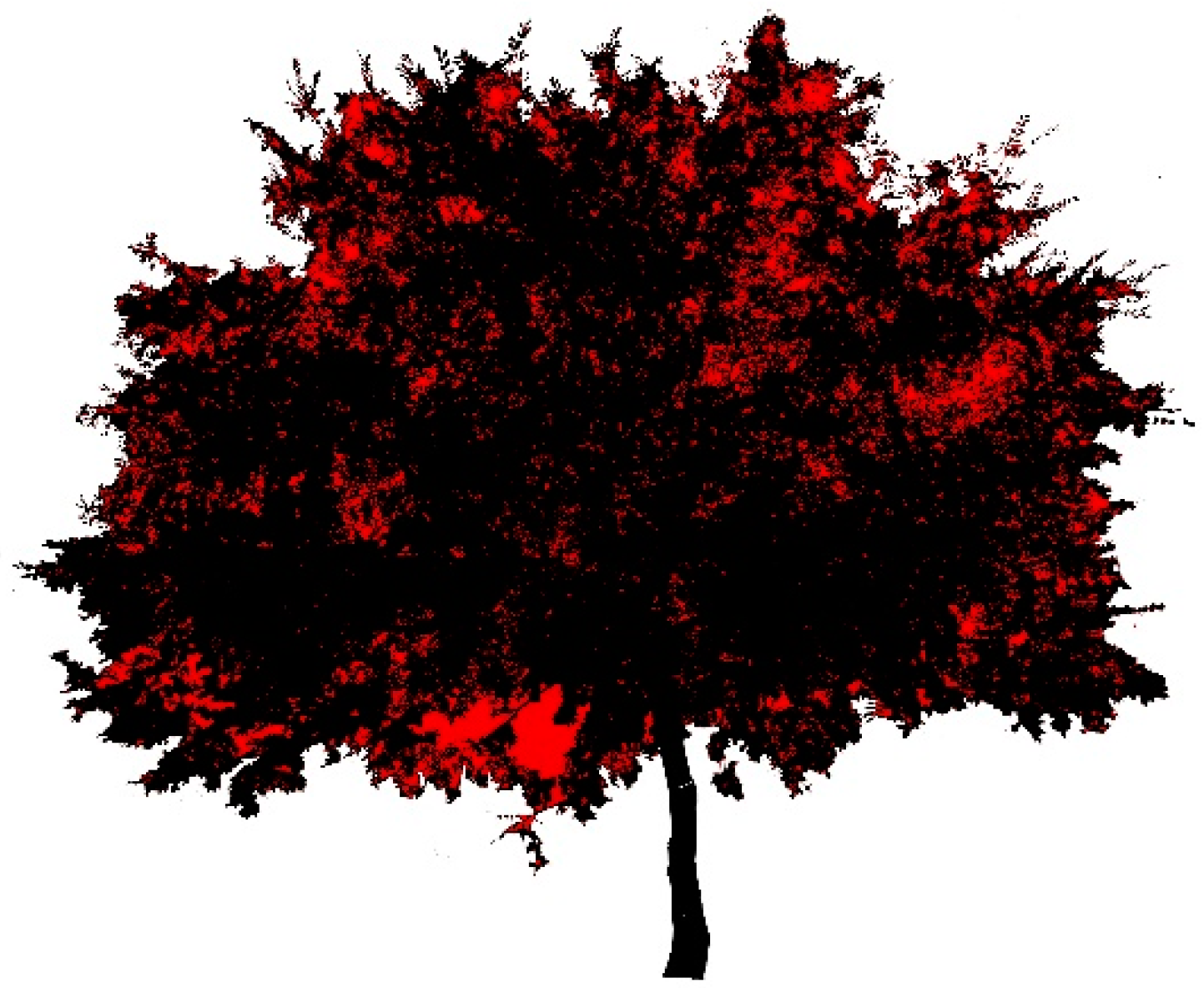
Referring to Miri’s [44] study defining the 2D porosity of a tree as the ratio of the tree’s pore area to its total area, the total 2D projected area of the canopy is equal to the 2D pore area plus the windward area, and the specific formula for the 2D porosity of a tree is given in Equation (12). According to the research of He and Li [24], the pore area of the tree photos by using the pixelation principle in Adobe Photoshop CS6 software is in line with the actual value, which proves that this method is highly feasible and accurate. The background area was then selected using the ’magic wand’ tool, and the total 2D projected area of the tree canopy was obtained by using the ‘inverse selection’ operation. Using the ’magic wand’ tool again, the canopy is selected to obtain the pixel value of its windward area. Finally, the required 2D pore area was obtained by subtracting the total 2D projected area of the canopy from the windward area of the canopy. Pixelated photographs of the trees are shown in Figure 8. In calculating the windward area, the trunk was selected as the scale, as the actual area of the trunk was relatively well determined. The actual value of the 2D pore area of the tree canopy was obtained according to Equation (13).

Since the actual path of air through a plant is different from light, which can only travel in a straight line, 2D porosity does not effectively capture the true effect of porosity on airflow. Grant and Nickling [30] demonstrated a strong relationship between the 2D porosity OP and the 3D porosity VP of the plant volume, with 2D porosity increasing as a power function of 3D porosity, as shown in Equation (14).

$$OP=\frac{A_P}{A_P+A_U}$$

(12)

$$\frac{X_D}{X_P}=\frac{A_D}{A_P}$$

(13)

$$OP=V{P}^{2.782}$$

(14)

where OP is the optional porosity, VP is the canopy porosity, A_P is the actual pore area, A_U is the actual frontal area at different wind speeds, X_D is the pixel value of the ruler, X_P is the pixel value of the pore, and A_D is the actual area of the ruler.

After pixelating the photos of the trees with Photoshop software, the 3D porosity values were obtained. Porosity, as one of the important tree characteristics, is significantly influenced by wind speed and direction, and the relationship between its variation and wind speed was explored.

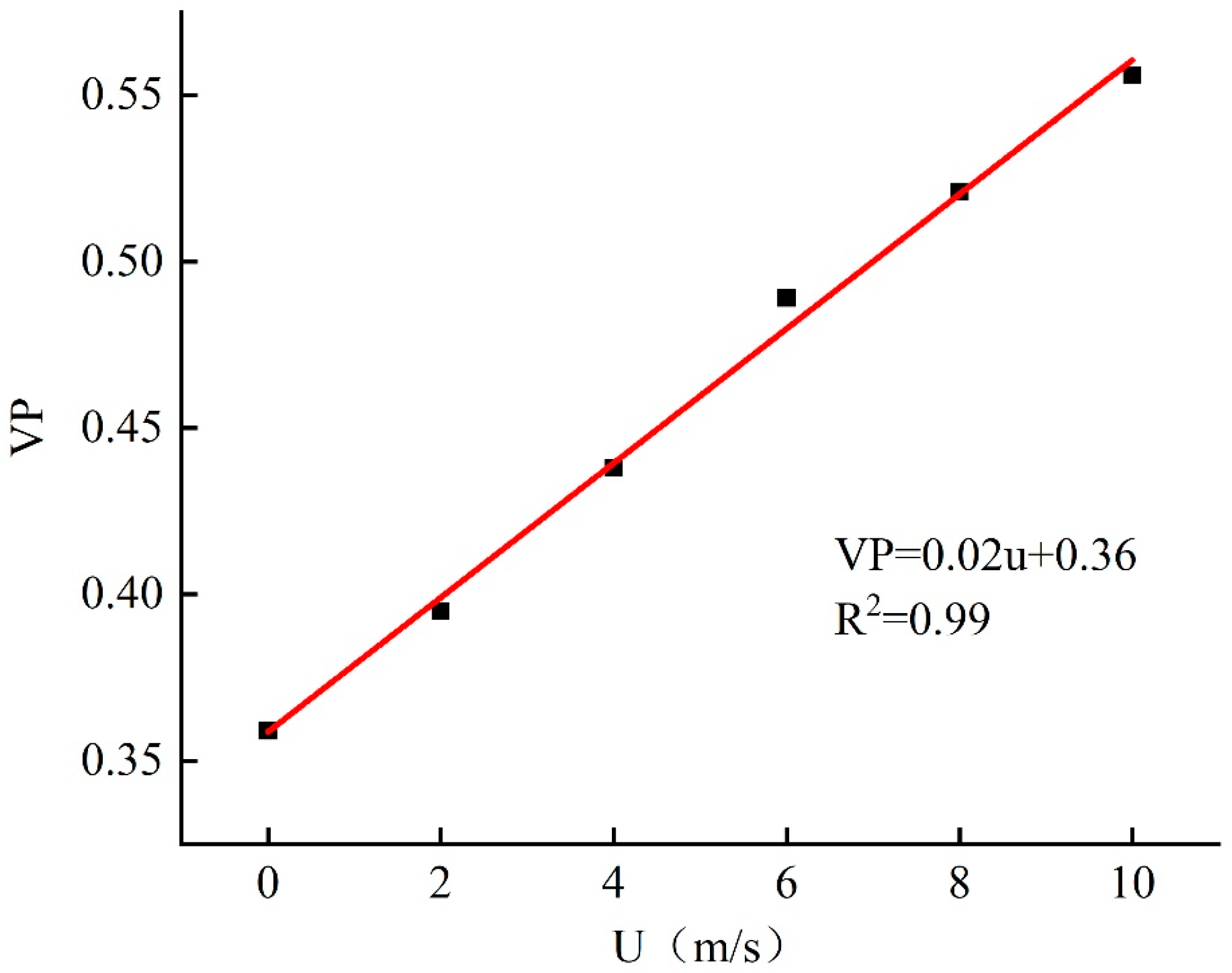
The effect of the wind on the tree will cause a change in the porosity and drag coefficient of the tree, which in turn will affect the flow of air through the leaves and branches of the plant through the control equation. A fitted relationship between the three-dimensional porosity VP and wind speed u was established by measuring the change in porosity at different wind speeds and is shown in Figure 9.

A linear function was used to fit the three-dimensional porosity and wind speed, and a functional relationship was obtained as VP = 0.02u + 0.36 and R² = 0.99. The correlation coefficient R² value of the fitted function was close to 1, proving that the fit was good. From the table and graphs, it can be seen that the tree porosity gradually increases with increasing wind speed under the same tree species. It is more difficult to obtain porosity at greater wind speeds, as the actual measurements are limited by uncontrollable factors, such as weather and wind speed, which are more demanding on natural factors and conditions. Therefore, by means of a fitted functional equation, the porosity can be calculated for any wind speed, and thus the drag coefficient can be obtained. This provides a more accurate simulation of the real changes in airflow through trees at different wind speeds and provides a reliable basis for subsequent experiments.

3.2. Measurement Process

The experimental instrument was selected from the Biaozhi digital wind speed and wind volume handheld anemometer GM8902+, as shown in Figure 10. The accuracy of the determination is ±3% ±0.1 dgts and the measurement range is 0 to 45 m/s. This instrument can record more than the basic stability, minimizing the degree of interference from other human factors, while referring to the methods of other scholars’ 500 strokes of data, which can be connected to a computer with USB for real-time remote monitoring.

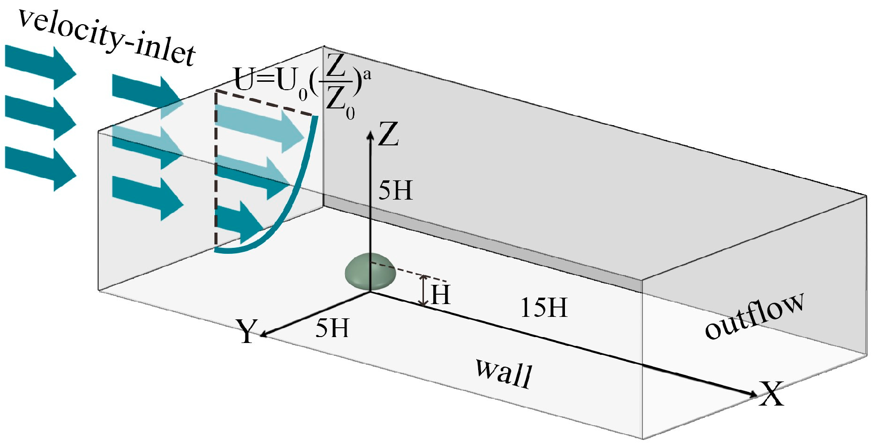
In the windward region of the tree and 0.5H, 1H, 1.5H, 2H, 2.5H and 3H in the downwind region, the monitoring points are arranged at heights of 1.7 m (0.25H), 3.4 m (0.5H), 5.1 m (0.75H) and 6.8 m (1H) from the ground. The locations of the monitoring points of the tree model are shown in Figure 11, with a total of 28 monitoring points.

The measured time is from 21 to 28 July 2022. Considering the obvious factors of wind force, the maximum wind speed occurs at noon every day. Therefore, the measurement period is a 1 h daytime period from 12:00 to 13:00. The main wind direction is east, and the wind force is five. The velocities at all monitoring points are synchronous and gathered in real time. All monitoring points record continuous data at five-second intervals over a one-minute period to obtain the average wind speed for that one-minute period. The above operation is repeated for three one-minute average wind speed tests, each three minutes apart. The wind speed at each monitoring point is the average of the three wind speed data points.

3.3. Verification Results

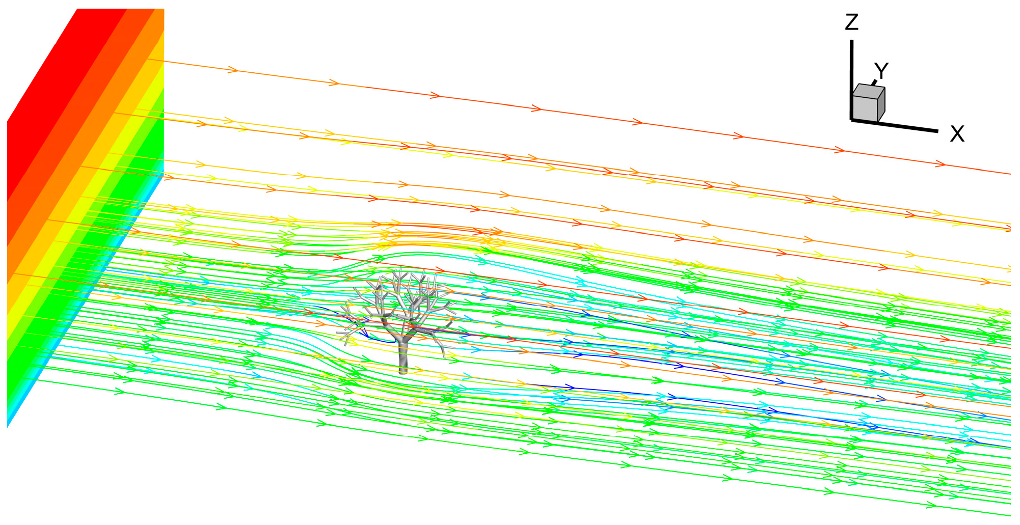
Figure 12 shows the 3D streamline of the flow field around the tree. The airflow follows the direction of the incoming wind and changes as it flows around the trees. Due to the obstructive effect of trees on the windward side of the airflow, part of the airflow passes through the tree canopy. The other part of the flow passes through the sides of the trees, above the trees and through the trunks of the trees.

Figure 13 shows the velocity of the fluid after passing through the canopy layer compared to the measured values, where the reference value is the simulation result of Rosenfeld [35]. The simulated results are shown as continuous black dashed lines, and the measured results are shown as solid red dots. The good agreement is in the range of 0.5~2H. The inaccuracy between the crown edge and the simulation increases at 2.5H and 3H farther from the tree. The wind direction in reality is not fixed and is accompanied by gusts. The farther away from the tree, the more likely the wind speed is disturbed, resulting in unstable wind direction and speed on the leeward side of the tree. In contrast, the wind speed flows at a steady rate from the windward direction of the trees in the numerical simulation. There is a certain error between the simulation and the measured results at a long distance. The reality of the environment also has interference with wind speed other than the instability of wind speed values and directions, including water and other trees. However, the overall trend in frontal areas and wind velocities leeward of tree e is generally consistent, so the experimental parameters can effectively reflect the airflow characteristics behind the tree.

Vogel [45] tested the change in resistance of a variety of plants at different wind speeds and demonstrated through extensive experimental studies that the resistance value of trees is a power function of the square of the wind speed, as shown in Equation (15).

$$\frac{F_D}{U^2}\propto U^E$$

(15)

where U represents the average wind speed and F_D represents the average resistance. E is the Vogel index (E < 0), the magnitude of which represents the deformation capacity of the tree under wind action.

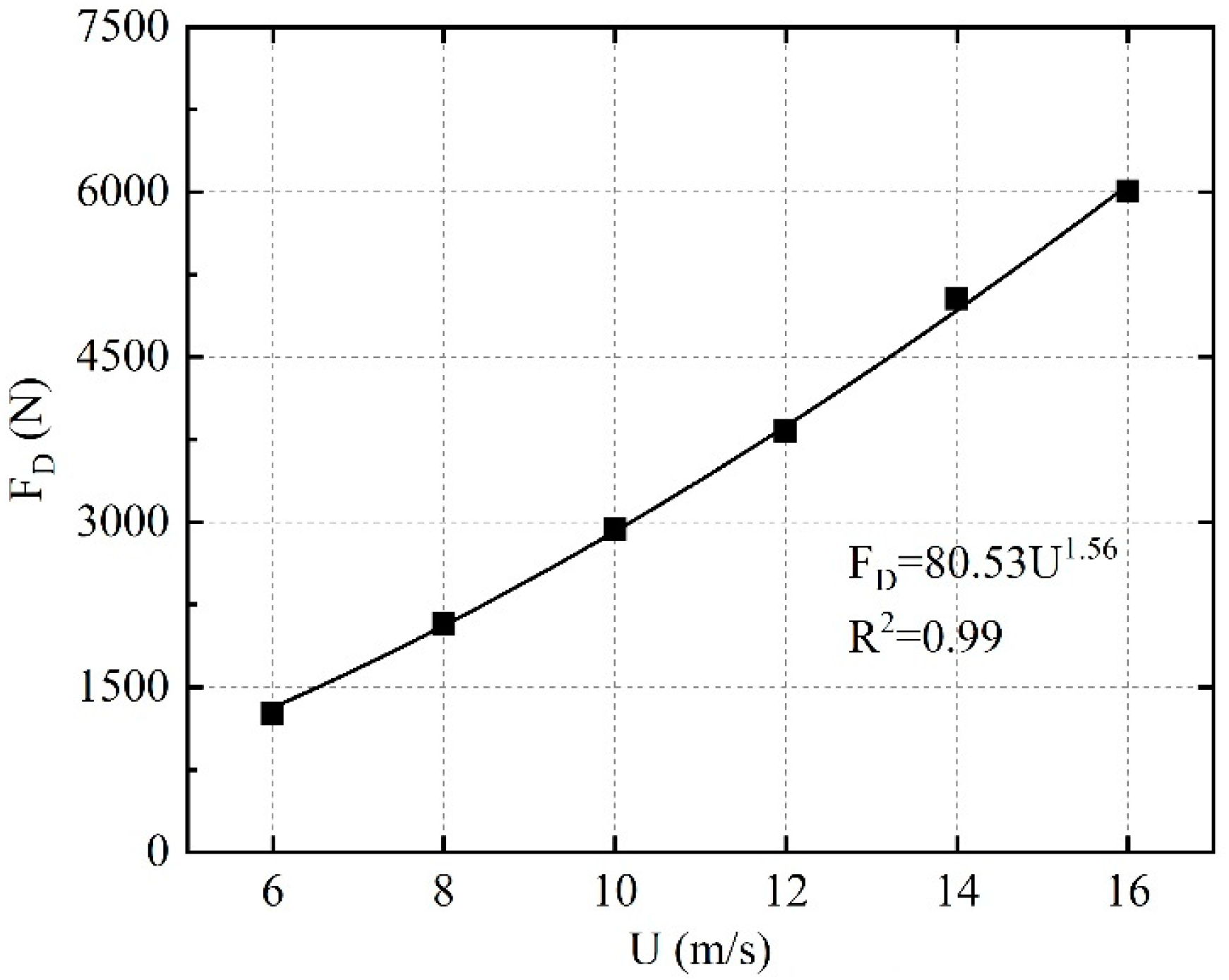
The higher the “E” value, the greater the deformation capacity of the canopy and the greater the bending by wind speed [22]. Manickathan et al. [26] showed that natural trees had “E” values between −0.18 and −0.51. Furthermore, the smaller natural trees experienced stronger deformation than the larger natural trees, possibly as a result of the reduced mechanical stiffness of their thinner branches. The model tree in this scenario has different deformation behavior at high wind speeds, so we calculated its resistance at different wind speeds, obtained a power function relationship between the resistance F_D and the wind speed U, are shown in Figure 14. And compared the “E” values of the model tree with the “E” values of the natural tree to verify the validity of the model tree.

The fitted curves of resistance and wind speed for the model tree in Figure 14 show that the power function relationship between resistance and wind speed for the trees numerically modeled in this paper is F_D = 80.53U^1.56, with an “E” of −0.44, which is within the “E” value for natural trees within the range of “E” values for natural trees. Therefore, the branch deformation capacity of the model tree is consistent with the results of natural tree research and is a good representation of the true force characteristics of the tree.

4. Parametric Study and Discussion

4.1. Force Characteristics of Trees

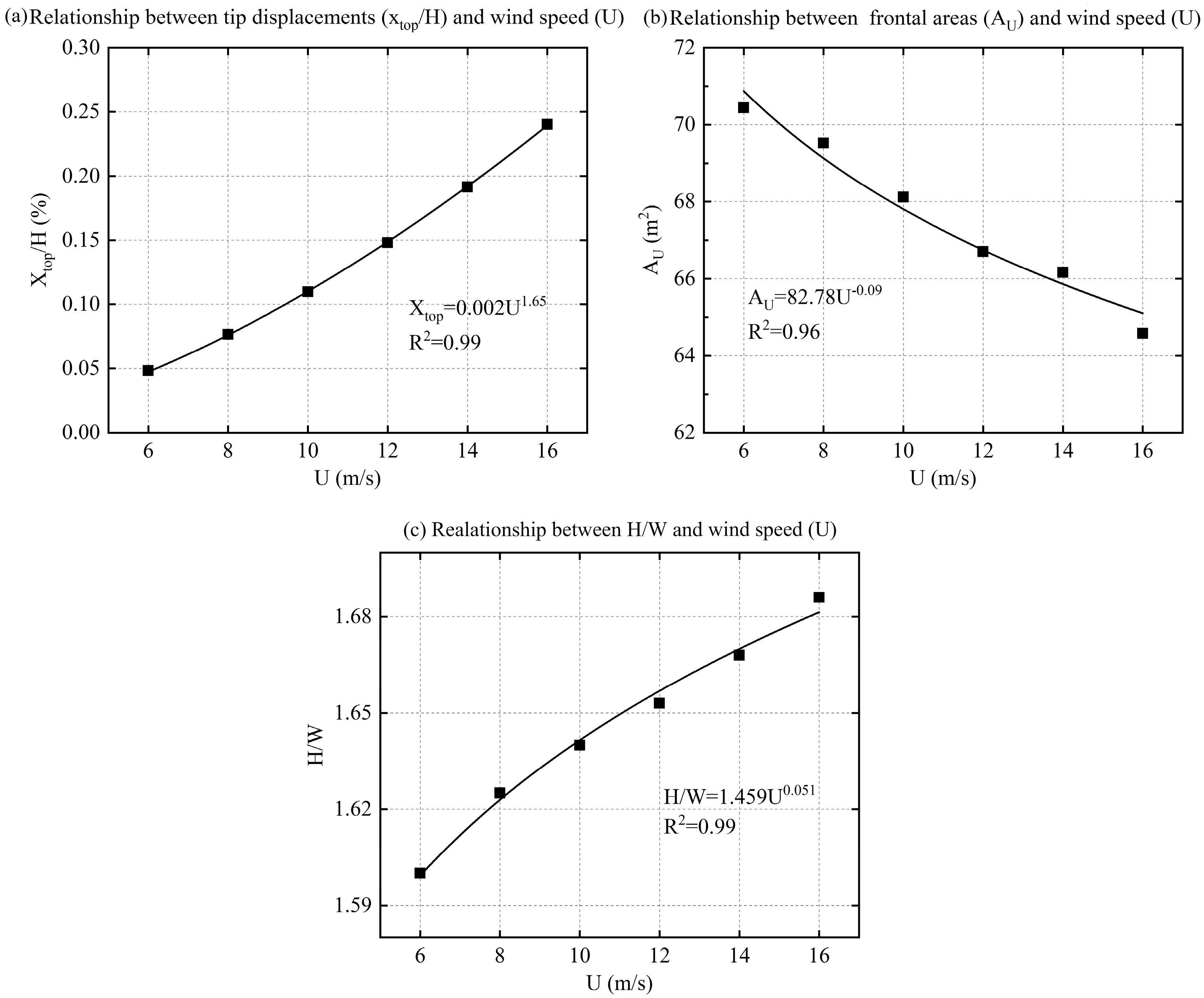
Power exponents were used to fit the top displacement and aspect ratio of the model tree to wind speed, and the fitted relationships are shown in Figure 14.

Normalized calculations for the tree tops by the tree heights. The top of the tree displacement and wind speed are fitted in Figure 15a. The normalized displacement of the tree top rises with increasing incoming velocities.

The windward area of the tree and the wind speed are fitted in Figure 15b, where it can be seen that the windward area decreases as the incoming velocity increases. When the incoming velocity rises from 6 to 16 m/s, the frontal area decreases by 9.42 m², representing 12.7% of the frontal area of the tree at rest.

4.2. Vertical Profile of the Flow Fields around the Tree

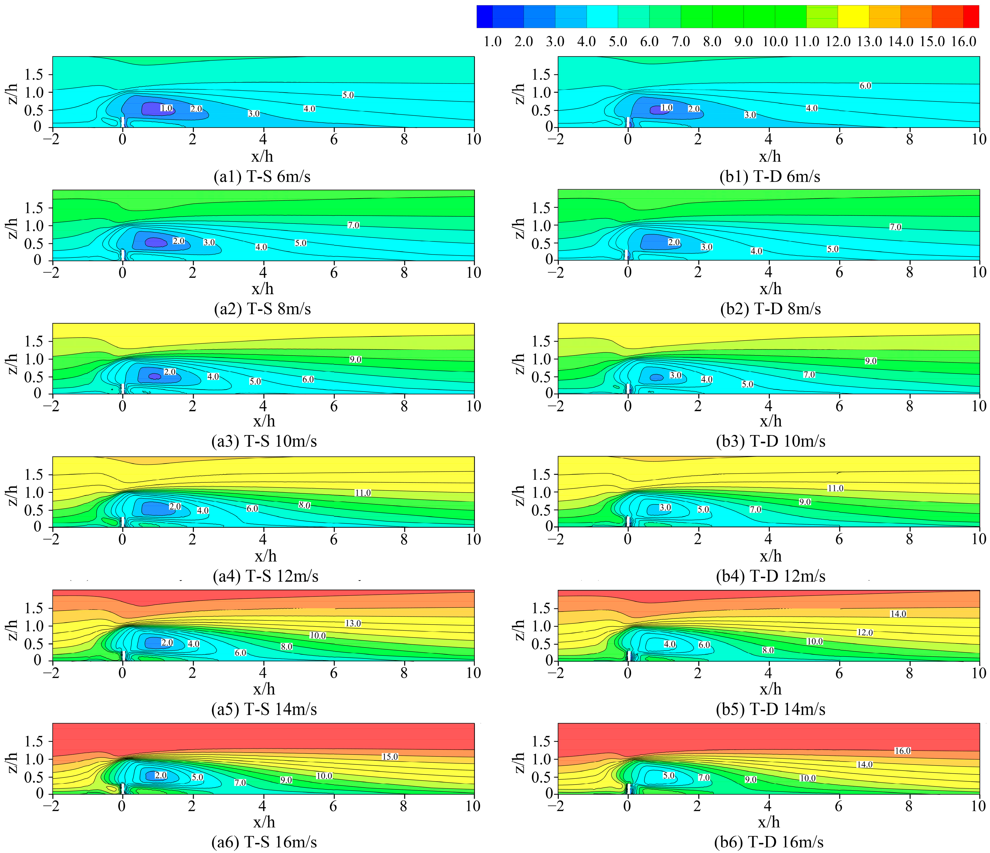
To investigate the effect of wind speed on the vertical flow field around a single tree, the vertical mean wind speed around the tree was analyzed for six control wind speeds of 6, 8, 10, 12, 14 and 16 m/s, are shown in Figure 16.

As shown in Figure 16, the trend characteristics of the vertical flow velocity distribution of trees in both T-S and T-D are the same, reducing the wind speed in the upwind and downwind areas due to the obstructive effect of trees on the airflow. There is a significant weakening of airflow in the upwind 1H range and in the downwind 7H range, forming a significantly weakened zone. However, trees still have a slight effect on the wind speed in the upwind range 1–2H and the downwind range 7–10, forming a slight deceleration zone.

The shape of both the T-S and T-D shelter zones is triangular, and the shape of the shelter zone is not influenced by tree deformation. When the stream velocity contours are slightly skewed, this indicates a slight recovery of wind speed into the stream. When the flow contours trend in a straight line, the wind speed has largely recovered. Eventually, a straight line will form at a greater distance, indicating that the flow has fully recovered to the inflow velocity and that trees no longer have an influence on the flow field. The progression of the contours from sloping to straight lines is the process of wind speed recovery.

As shown in

Table 2. Area of tree shaded areas.

u	6 m/s	8 m/s	10 m/s	12 m/s	14 m/s	16 m/s
T-S	2.5H	2.8H	3.0H	2.5H	2.7H	2.8H
T-D	2.2H	2.4H	2.4H	2.4H	2.5H	2.5H

, the minimum wind speed in the sheltered area behind the tree increases with increasing control wind speed for T-S and T-D at an average distance of approximately 2.7H. The range of the sheltered area is reduced by 0.3H for T-D compared to T-S. Additionally, as seen from the graph, the minimum wind speed in the sheltered area behind the tree increases with increasing control wind speed. In the T-S case, the minimum flow velocity in the sheltered area increases slightly from 1 m/s at an incoming wind speed of 6 to 2 m/s at an incoming wind speed of 16 m/s, with a difference of 1 m/s. In the T-D case, the minimum flow velocity in the sheltered area increases significantly from 1 m/s at an incoming wind speed of 6 to 5 m/s at an incoming wind speed of 16 m/s, with a difference of 4 m/s. The minimum flow velocity increases faster in T-D than in T-S. The trend of increasing flow velocity is faster than that of T-S. This demonstrates that the deformation of the tree with increasing wind speed increases due to increased porosity and airflow through the flow. As a result, the wind response of the tree to airflow is significantly weaker and less intense.

The relative wind speed change trend of the deformed trees is the same at 1H of the downwind area under different control wind speeds in Figure 17. When the relative height is 0–0.5H, the relative wind speed decreases with increasing height. When the relative height is 0.5–1.4H, the relative wind speed increases with increasing height and reaches the minimum value at approximately 0.5H, which is the height of the maximum canopy width, indicating that the slowing effect is most pronounced in the center of the canopy.

The relative wind speed curve progressively moves to the right as the control wind speed rises, and the lowest relative wind speed rises from 0.17 at 6 m/s to 0.31 at 16 m/s. This is because when the incoming velocity rises, the deformation of the canopy will affect the airflow through the tree and the resulting drag coefficient, reducing the sheltering effect on wind speed behind the tree. This phenomenon is also found in field measurements of mature trees.

When the relative height is at 0–0.5H, the turbulence intensity shows an increasing trend with the increase in height. At the relative height of 0.5–1.4H, the turbulence intensity tends to decrease with the increase in height, and the maximum turbulence intensity was reached at the center of the canopy at 0.5H. The turbulence intensity is gradually shifted to the left with increasing wind speed relative to the reference point in the canopy height range.

4.3. Horizontal Profile of the Flow Fields around the Tree

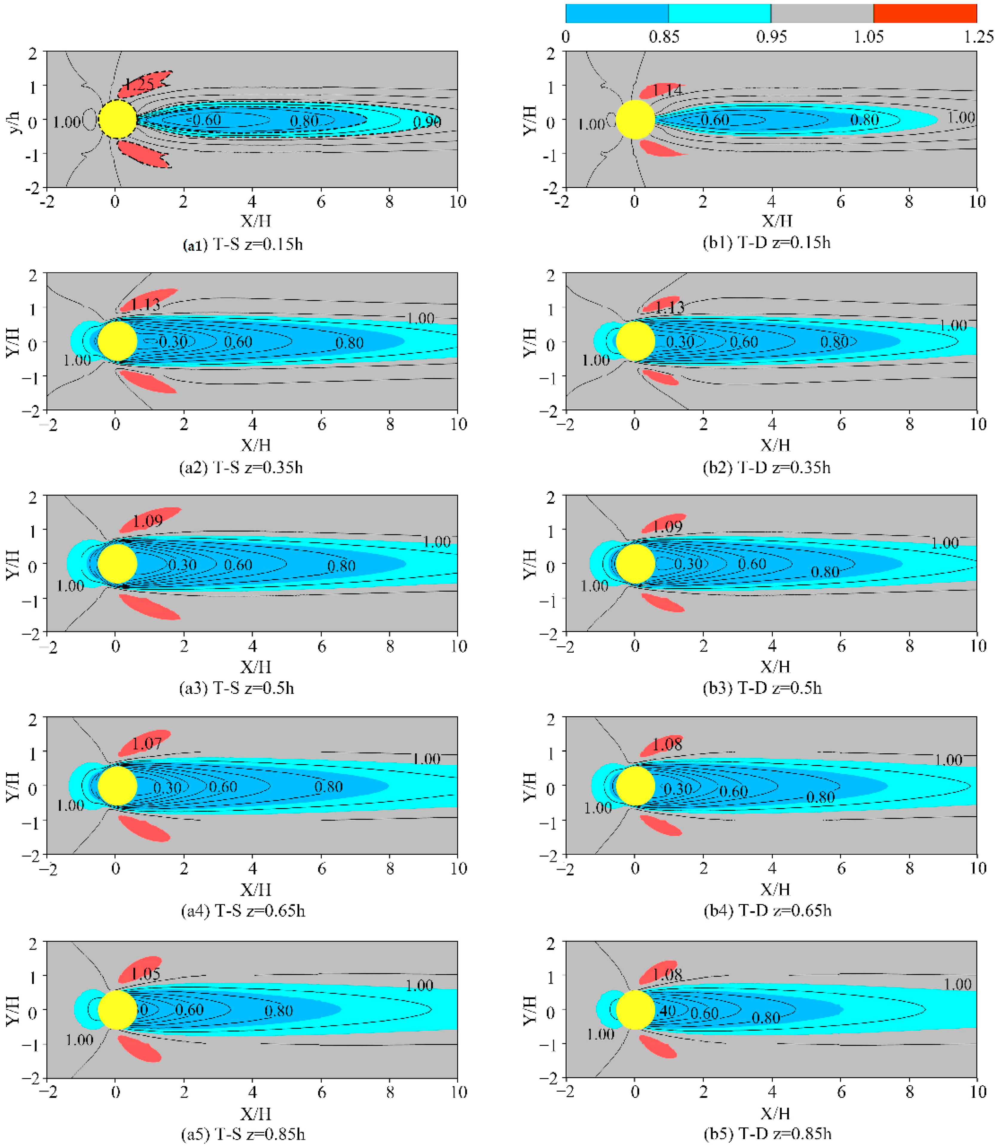
The airflow is divided into four levels to make it easier to identify the form and size of each partition. These levels are as follows: strong deceleration in navy blue (u_re < 0.85), weak deceleration in baby blue (0.85 < u_re < 0.95), acceleration in red (u_re > 1.05), and no effect in gray (0.95 < u_re < 1.05), as shown in Figure 18. The inflow velocity is 6 m/s.

As shown in Figure 18, a light blue oval weak deceleration zone and a few dark blue strong deceleration zones were formed in the upwind and downwind areas of the trees. The dark bule strong deceleration zones were only formed at the wide crown width in the upwind areas. The deceleration range of the upwind direction is small in the range of −1~0 h, and the speed is reduced between 5% and 15%. The trees have an obvious shielding effect on the downwind direction from the size of the dark blue and light blue deceleration zones in the downwind direction, and the deceleration range of the weak deceleration zone can reach 10H. The range of strong deceleration extends to approximately 6–8H, and the wind speed decreases obviously in this range. The range of the deceleration zone of deformed trees decreases by approximately 0.5H compared with stationary trees at the same height. This indicates that the shielding effect of deformed trees on wind speed decreases. The airflow acceleration was observed on both sides of the trees at different heights. With the increase in height, the acceleration effect on both sides was weaker. The relative velocity value of deformed trees decreased from 1.14 to 1.08, indicating that the porosity of the deformed trees increased, and the blocking and squeezing effects on the airflow decreased.

The difference in canopy width leads to the difference in airflow field partition area at different heights. The 0.15H value is the height of the trunk, which has a significantly smaller effect on the airflow velocity than other heights within the range of crown width. The maximum width of trees is at 0.45H, so the wind speed is obviously weakened in a2 and a3 and the width of deceleration zone in a3 is larger than that in a2, so the weakening effect of 0.5H height on wind speed is the most significant. The width of the tree canopy gradually decreases from 0.5H to the top of the tree. The area of the blue area in the graph, therefore, also decreases, indicating a reduced weakening effect on wind speed. In a1~a5, the largest red acceleration area is in a3, and the acceleration area of adjacent height a4 is relatively reduced by 7.9%. The red acceleration area of b1~b5 is significantly smaller than that of a1~a5. Although the red acceleration area of b3 is still the largest, the acceleration area of b4 relative to a3 is reduced to 2.5%. The reason may be that the deformation of trees has a significant effect on the maximum canopy width, and the width changes at other heights are relatively small.

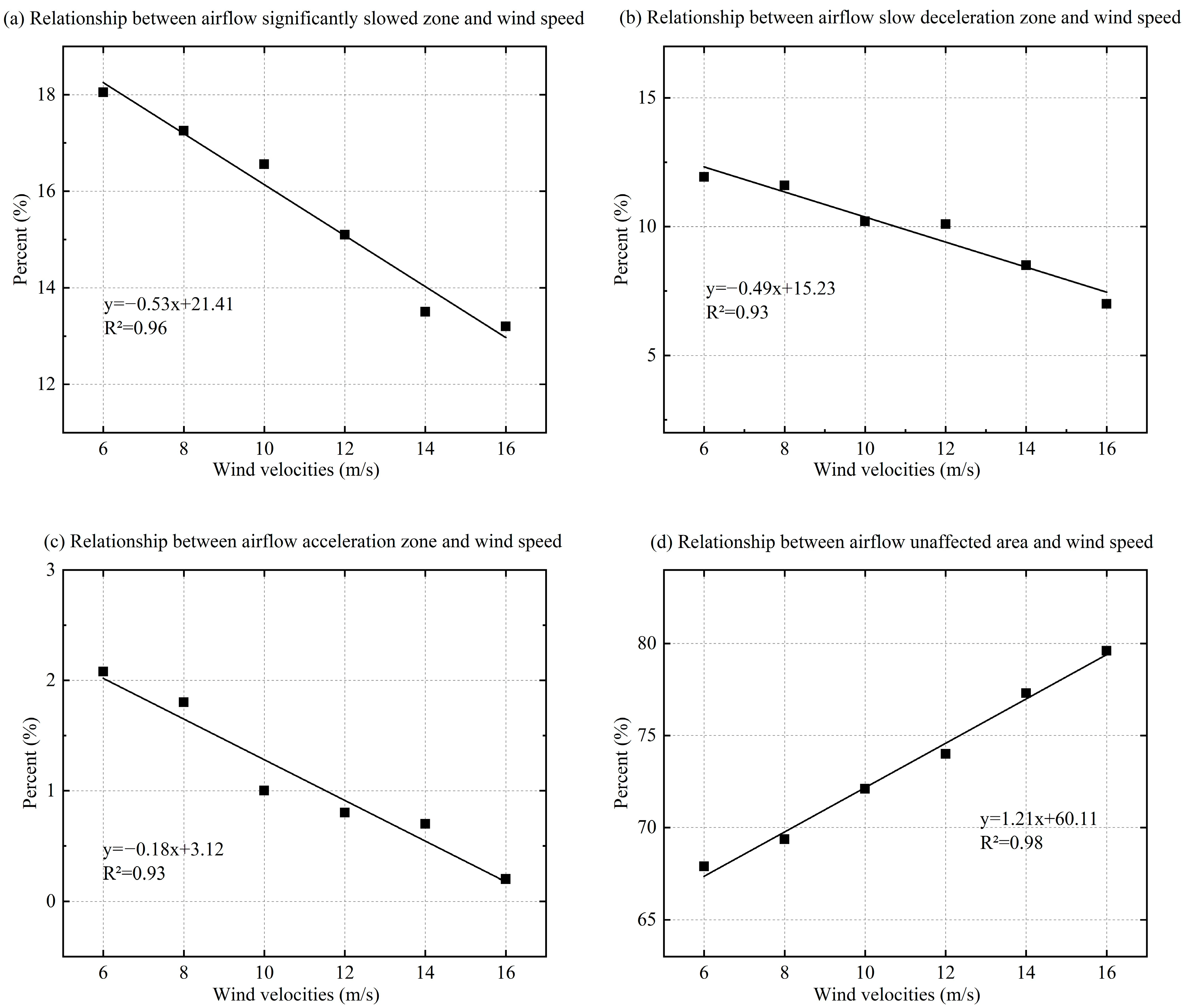
The unaffected zone accounts for over 70% of the total area, as shown in Figure 19d; the strongly weakened zone accounts for approximately 15%, as shown in Figure 19a; the weakly weakened zone accounts for approximately 10% of the total area, as shown in Figure 19b; and the accelerated zone accounts for less than 2%, as shown in Figure 19c. The area of all zones varies with wind speed. Except for the unaffected zone, the area of all zones decreases as the wind speed increases. There is a clear correlation between the area of the different zones and the velocity. The unaffected zone has the greatest correlation (R² = 0.98), and the strongly weakened zone has a slightly greater correlation (R² = 0.96) than the weakly alkaline speed zone (R² = 0.93). As the incoming wind speed increased from 6 to 16 m/s, the area of the strongly weakened zone decreased from 18% to 13%, and the area of the weakly weakened zone decreased from 12% to 7%. Both of their area shares decreased to 5%, and the sum of the weakened zone areas decreased by 10%. It follows that for every 1 m/s rise in the incoming velocity, the sum of the weakened areas decreases by approximately 1%. The change in the area of the acceleration zone is the smallest, with a decrease of less than 2%.

4.4. Effect of Changes in Tree Characteristics on Airflow Parameters

It is clear from previous studies that the recovery process of airflow in the downwind deceleration zone is determined by plant characteristics. Trees are deformed by wind forces, and tree characteristics, including height-to-width ratio and porosity, are altered. The deformation of trees under different incoming wind speeds causes changes in the characteristic parameters of the tree height-to-width ratio and porosity, as shown in

Table 3. Variation in tree character parameters.

u	6 m/s	8 m/s	10 m/s	12 m/s	14 m/s	16 m/s
VP	0.489	0.521	0.556	0.589	0.612	0.634
H/W	0.794	0.806	0.820	0.826	0.834	0.843

.

As shown in Table 3, the pore space of the trees increased with increasing wind speed, from 0.489 at 6 m/s to 0.634 at 16 m/s. Both the height and width of the trees decreased with increasing wind speed, while the height-to-width ratio increased with increasing wind speed, from 0.794 at 6 m/s to 0.843 at 16 m/s.

Cheng et al. [13] showed that the recovery of airflow over the leeward side of the plant is modeled as follows:

$$f\left(x\right)=u_0-\left(u_0-u_{min}\right)exp\left(-\frac{x-x_0}{l}\right)$$

(16)

where u₀ (m/s) is the incoming velocity, u_min (m/s) is the minimum speed, x₀ (m) is the location of u_min, and l (m) is the length of the recovery feature and represents the distance from the wind speed on the leeward side of the plant to recover to 1−exp(−1) of the lost wind speed [13]. The variation in the airflow model parameters u_min, x₀ and l after the wind response of trees at different wind speeds in this paper is shown in

Table 4. Variation of airflow model parameters.

u	6 m/s	8 m/s	10 m/s	12 m/s	14 m/s	16 m/s
x0/H	0.841	0.831	0.771	0.802	0.761	0.752
umin = u/u0	0.164	0.189	0.221	0.251	0.274	0.301
l/H	5.038	4.929	4.699	4.529	4.468	4.309

.

Table 4 shows that u_min increases with increasing wind speed, from 0.164 at 6 m/s to 0.301 at 16 m/s; x₀ decreases with increasing wind speed, from 0.841 at 6 m/s to 0.752 at 16 m/s; and l decreases with increasing wind speed, from 5.038 at 6 m/s to 4.309 at 16 m/s. Thus, the downwind sheltering effect and the range of influence of the trees after the occurrence of wind-induced response are weakened, the minimum velocity value u_min behind the trees increases, the distance to its occurrence location x₀ decreases and the distance required to recover the same air velocity is reduced.

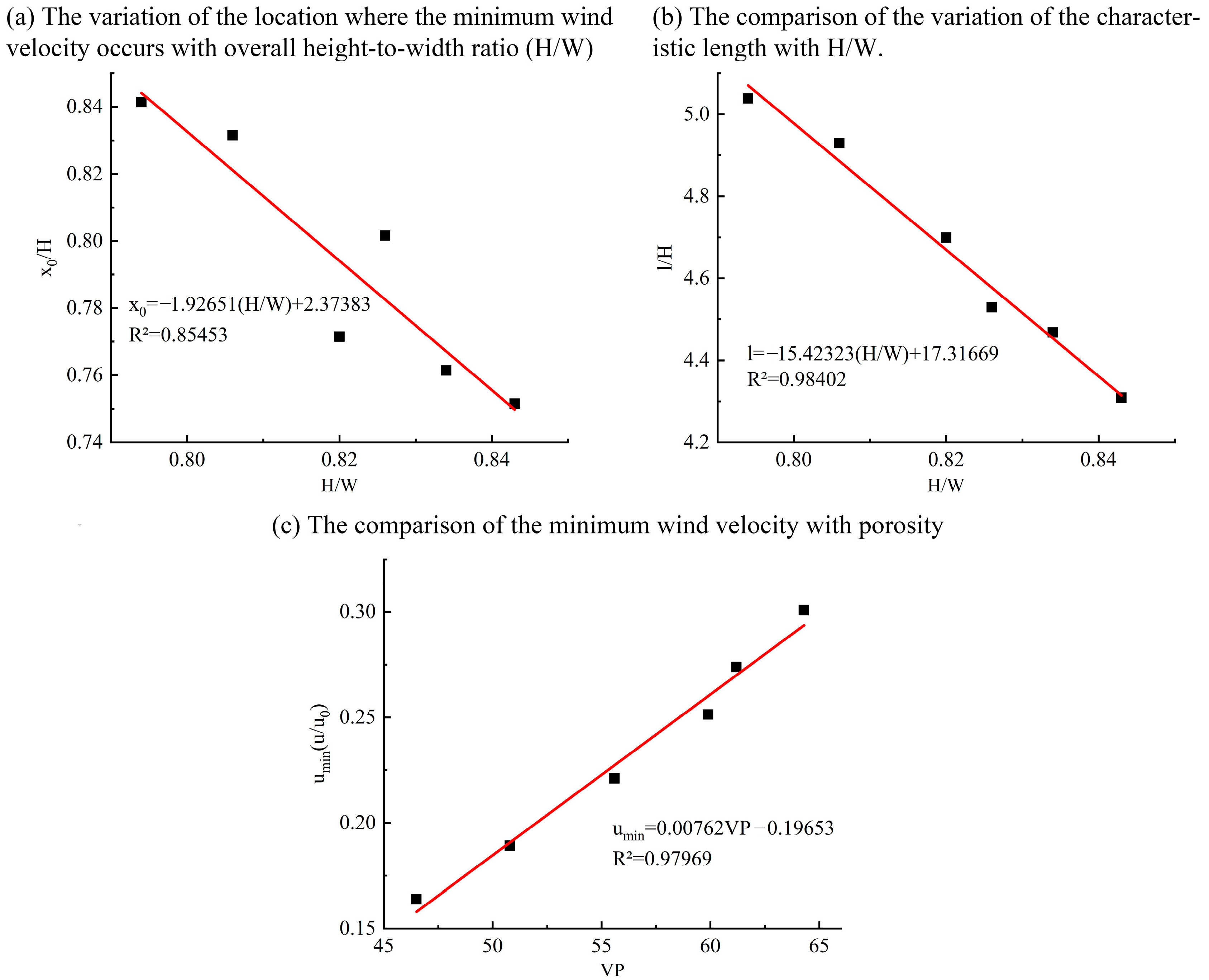
Based on multiple regression analysis, the tree characteristic parameters with significant correlations and effects on u_min, x₀, and l and their best-fit relationships were derived in Figure 20.

The x₀ values for the leeward areas of the trees and the l values for the length of the airflow recovery features differ significantly for different heights and widths of plant characteristics. The fitted correlation between the value of x₀ and H/W is linearly negative in Figure 20a. The reason for this phenomenon is that the airflow through the plant requires a long weakening process when the H/W is small. The width of the tree will affect the distance required for the lateral airflow to reach the rear side of the tree. Therefore, the minimum wind speed behind the tree forms further away from the tree. For trees with larger H/W, the downwind airflow of the tree will be affected by the downwind airflow of the treetop, which will accelerate the flow and reduce the distance where the minimum velocity occurs. The u_min in the leeward area of trees generally occurs within 3H of trees. The value of l is linearly negatively correlated with H/W in Figure 20b. In their study of trees with similar H/W but noticeably varied porosities, Cheng et al. [13] discovered that the length of the airflow recovery was unrelated to plant porosity, which was primarily determined by H/W.

The value of the minimum wind speed u_min in the downwind area of the tree is significantly different for the different porosities. The value of u_min is linearly positively correlated with VP in Figure 20c. This phenomenon is caused by the more flexible leaves and tiny branches of the canopy being impacted by the wind speed and reoriented along the wind direction as the incoming velocity rises. The effect of branches and leaves on the disturbance of air currents through the canopy is relatively weak. At the same time, the porosity rises concurrently with a decrease in the overall tree’s ability to prevent airflow and an increase in airflow via the tree’s pores. Therefore, the porosity determines the ratio of airflow through tree pores to airflow divergence above and around trees. The porosity increase in deformed trees leads to an increase in airflow u_min.

In summary, the windproof distance and effects of deformed trees also change with different wind speeds. The reason for the differences is that the tree characteristics are changed by different wind speeds, which has an impact on the surrounding flow field. The H/W affects the weakening process, and the porosity determines the airflow ratio through the trees and the resulting drag coefficient.

5. Conclusions

In this study, to simulate the deformation state of trees under wind forces, a deformed porous model describing the external contour of branches is established. The change in the drag coefficient under different wind speeds is considered. The influences of deformed trees on the surrounding flow field of trees are studied. The measurement of wind velocities around a single tree is performed. The simulated results are in good agreement with the measured results. The findings of this study are as follows:

(1)

The general trend in velocity distribution and flow structure was consistent for both T-D and T-S. The shape of the shelter zone behind the trees is all triangular, but the wind response reduced the extent of the wind shelter zone of the trees by 0.3H. The distance at which the trees had a significant sheltering effect on wind speed was 2.4H. As the wind speed increased, the difference in the wind environment between wind-responsive trees and vertically fixed trees gradually increased, and the difference in the minimum wind speed values behind the trees increased.

(2)

The partition of the surrounding flow field mainly includes the acceleration zone on the sides, the weakened zone downwind and the mild deceleration zone upwind due to the shelter effect of trees. The deceleration in the downwind direction can be extended to 7H, and there is still a slight effect after 7H. The most obvious effect on the weakening of wind speed is 0.5H, where the canopy width is the largest. The sum of the weakened areas decreases by approximately 1% for every 1 m/s rise in the incoming velocity.

(3)

Quantifying the effect of changes in porosity and aspect ratio on the wind environment due to wind-induced response. The relationship between porosity and minimum wind speed is u_min = 0.00762VP − 0.19653, and the relationships between the aspect ratio and minimum wind speed occurrence location x₀ and wind speed recovery distance l are x₀ = −1.92651H/W + 2.37383 and l = −15.42323H/W + 17.31669, respectively.

(4)

The degree of variation in flow velocity is most pronounced within the height and width of the canopy as the incoming wind velocity increases. At the same distance behind the tree, the relative flow velocity curve of wind-responsive trees gradually shifts to the left, and the flow velocity increases as the incoming wind velocity increases. As the distance behind the tree increases, the effect of the change in tree characteristics due to the wind response of the tree decreases.