Article

Evaluation of PBL Parameterization Schemes in WRF Model Predictions during the Dry Season of the Central Amazon Basin

by
José Antonio Mantovani Júnior
*,
José Antonio Aravéquia
,
Rayonil Gomes Carneiro
and
Gilberto Fisch
National Institute for Space Research (INPE), Av. dos Astronautas, São José dos Campos 12227-010, SP, Brazil
*
Author to whom correspondence should be addressed.
Atmosphere 2023, 14(5), 850; https://doi.org/10.3390/atmos14050850
Submission received: 27 March 2023 / Revised: 20 April 2023 / Accepted: 25 April 2023 / Published: 10 May 2023
(This article belongs to the Special Issue Atmospheric Boundary Layer Modeling and Observation)

Abstract

:
Planetary Boundary Layer (PBL) parameterization schemes are employed to handle subgrid-scale processes on atmospheric models, playing a key role in accurately representing the atmosphere. Recent studies have shown that PBL schemes are particularly fundamental to the depiction of PBL height (PBLH), especially over the Amazon. In the present study, we investigated the performance of PBL schemes on the representation of meteorological variables, turbulent fluxes, PBL vertical structures, and PBLH over the central Amazon basin under dry conditions, taking advantage of observations from the Observations and Modeling of the Green Ocean Amazon campaign (GoAmazon2014/5) for validation and evaluation. Numerical experiments were carried out within the WRF model using eight PBL schemes for two dry periods from 2014 (typical year) and 2015 (El-Niño year), and results from the 1-km resolution domain were directly compared to hourly in situ observations. In general, all PBL schemes present good performance to reproduce meteorological variables, with nonlocal (local) PBL schemes producing better performance in the 2014 (2015) study period. All PBL schemes in general overestimate (>100%) daytime turbulent fluxes. Thermodynamic (daytime) vertical structures are better predicted than mechanical (nocturnal) ones. The local MYNN2.5 scheme showed the overall best performance for PBLH prediction, mainly at night.

1. Introduction

Accurate prediction of Planetary Boundary Layer (PBL) parameters has been recognized as critical due to its effects on short-term weather forecasting and long-term climate simulations, and it is also required to achieve realistic pollutant dispersion simulations and air quality prediction [1,2]. Numerical Weather Prediction (NWP) models make use of a PBL parameterization scheme to handle the subgrid-scale turbulent processes within the PBL and free atmosphere, since it is unfeasible and expensive to fully resolve all scales of turbulence [3]. Therefore, the PBL parameterization scheme affects the accuracy of predicted PBL height (PBLH) and other meteorological parameters, leading to significant differences in predicted variables [4]. PBL schemes are considered the major source of uncertainty in NWP models [3,5]. Recent studies have highlighted the significance of model validation with observational data and the development of sensitivity studies to optimize model setup [4,6], especially regarding PBL schemes due to the impacts on Weather Research and Forecasting (WRF) model calculations [7,8].
PBL parameterization schemes have improved over the last decades, covering different atmospheric stability regimes, PBL features, mixing approaches, and numerical techniques [9,10,11,12,13,14,15,16,17]. These schemes are classified based on the order of turbulence representation and mixing treatment. For instance, local PBL schemes assume vertical transport only between adjacent model layers and are indicated to work better under stable stratification due to the local mixing associated with small eddies, while nonlocal PBL schemes allow the transport between distant layers and perform better under unstable stratification to account for the effect of larger eddies [18]. The impacts of PBL schemes on different studies were the subject of several works [19,20,21,22,23]. Different PBL schemes were tested using the WRF model under a wide range of model versions, meteorological conditions, atmospheric processes, and methodologies in the past few years [24,25,26,27,28].
Even though several studies have evaluated the performance of PBL schemes in North America, Europe, and Asia [29], there are relatively few studies on the performance of PBL schemes to depict the Amazonian PBL [30,31,32]. Wang et al. [30] investigated the sensitivity of land–atmosphere coupling strength to boundary and surface layer parameters over the Amazon during the wet season using a nonlocal PBL scheme through WRF model simulations with 50-km horizontal resolution. Their results showed that simulations could roughly capture the observed daily cycles of surface variables and turbulent heat fluxes, while the PBLH is underestimated at night. Afterwards, Wang et al. [31] quantified the physical parameterization uncertainties and evaluated six PBL schemes during the wet season following the model setup from Wang et al. [30], whose results indicated that diurnal PBLH is better predicted than its nocturnal counterpart. In a different approach, Prein et al. [32] simulated tropical mesoscale convective systems under convection-permitting resolution (4-km) in the Amazon basin, and results showed that a nonlocal PBL scheme performed better in comparison to a local PBL scheme. These studies have provided significant results regarding the performance of PBL schemes over the Amazon so far, but, on the other hand, they are limited in terms of simulations (analysis or reanalysis as initial conditions), model horizontal resolution (50 and 4-km), as well as the season of the year (mostly wet season).
The boundary layer over the Amazon rainforest during the dry season has been studied in the past [33], where the NASA Amazon Boundary Layer Experiment provides investigation regarding the structure and evolution of the daytime mixed-layer under undisturbed conditions. The Amazonian boundary layer during the dry season exhibits a strong diurnal cycle that is coupled to the surface during the daytime and uncoupled at nighttime with the formation of a stable boundary layer (SBL) about 300 m deep, while the PBLH can reach 2000 m over pasture sites in the afternoon [34]. The Observations and Modeling of the Green Ocean Amazon field campaign (GoAmazon2014/5) took place in the central Amazon basin between 2014 and 2015 and collected an unprecedented data set with aircraft flights, in situ measurements, and several instruments to gather detailed atmospheric observations [35].
Among studies that investigated the PBL with GoAmazon2014/5 datasets, Henkes et al. [36] indicate that the development of Amazonian PBL during the dry season typically occurs in four stages: the nighttime stable stage (21–06 Local Time—LT, LT for the Amazon basin is UTC—4 h), the morning transition stage (06–08 LT), the rapid growth stage (starting around 08–09 and ending at 11 LT), and the cloudy mixing layer stage (11–15 LT). Carneiro and Fisch [37] investigated the development of PBL depth through measurements from several instruments and found that the ceilometer provides accurate and continuous measurements of the PBLH. They also found that the influence of the El Niño southern oscillation (ENSO) during the 2015 year increased the daytime PBL depth by 21% compared to 2014 (considered a typical year). In terms of modeling, previous studies [30,31] identified that the choice of PBL schemes is significant for PBLH simulation, especially at nighttime. Moreover, the appropriate depiction of nocturnal stable and morning transition stages is crucial to reproduce adequately the daytime PBL development [38].
In this study, we evaluate the performance of eight PBL schemes in short-term forecasts using the WRF model over the central Amazon basin for the 2014 and 2015 dry periods. GoAmazon2014/5 in situ observations of meteorological variables, turbulent fluxes, PBL vertical structures, and PBLH are analyzed and directly compared to 1-km resolution forecasts to validate the numerical experiments and evaluate the performance of tested PBL schemes. The main goal of the present work is to investigate the impact of PBL schemes on the prediction of referred parameters under undisturbed conditions to identify model biases and the overall performance of these schemes to represent the development of PBL depth. Both nonlocal and local PBL schemes were evaluated, and the main differences are presented and discussed, as well.

2. Materials and Methods

2.1. Study Area and Observational Data

The observations from the GoAmazon2014/5 field campaign were used for model validation in the present study. These data were collected at a research site named T3 (3.213° S, 60.598° W, 50 m) located nearby the confluence of the Negro and Solimoes rivers in Manacapuru City, Amazonas, Brazil (Figure 1a). The measurements were made for 24 months during the 2014 and 2015 years through Atmospheric Radiation Measurement (ARM), Mobile Facility One (AMF-1) and the ARM Mobile Aerosol Observing System (MAOS) [39]; further details about the meteorological and background conditions can be found in the literature [35,37]. In short, the 2014 year was a typical year with precipitation rates similar to normal climatology, while the 2015 year was characterized by the intense ENSO event producing reduction in precipitation rates (30% in comparison to 2014), generating pronounced dry conditions [37].
In the present research, the performance of eight PBL schemes is evaluated using detailed observations of the 2014 and 2015 dry season periods, specifically from 30 September to 2 October 2014, as well as from 14 to 16 October 2015. These periods were selected due to occurrence of Intensive Operating Periods (more data is available) and the observed conditions; for the selected 2014 period, there is the presence of isolated convective rain typical of the dry season, while, for the 2015 period, there is no presence of rainfall. The near-surface meteorological variables from the Meteorological Measurements Associated with the Aerosol Observing System (AOSMET) [40], which correspond to 2-m air temperature (T2), 2-m air relative humidity (RH2), 10-m horizontal wind speed (U10), and precipitation (PCP), are compared to predicted ones. The predicted turbulent fluxes were validated using measurements of eddy covariance fluxes, such as friction velocity (u*), sensible heat flux (H), and latent heat flux (LE), collected by the Eddy Correlation Flux system (30ECOR) [41]. Regarding PBL conditions, the atmospheric vertical profiles for potential temperature (θ), vapor mixing ratio (q), and horizontal wind speed (U) collected through radiosonde soundings launched over the T3 site (SONDEWNPN) [42], which are available at 02, 08, 14, and 20 LT, were compared to the predicted ones.
Regarding the PBLH data, the observed PBLH is retrieved from continuous ceilometer measurements (CEILPBLHT) [43] with high temporal resolution (16 s), which provides the complete diurnal cycle of the PBLH. A CL31 ceilometer from Vaisala Inc. (Finland) was installed as part of the GoAmazon2014/5 campaign, capable of operating at a maximum vertical range of 7700 m. This instrument records the intensity of optical backscattering within a near-infrared wavelength range of 900 to 1100 nm by autonomously emitting a vertical pulse [37]. Pulsed diode laser lidar (light detection and ranging) technology is utilized by ceilometers to determine the attenuated backscatter, from which particle backscatter coefficients can be derived. Using this data, the heights of the cloud base and the PBL can subsequently be calculated [44,45,46]. From these measurements, several derived products are obtained, including the height of the cloud base, the particle backscatter coefficient retrieval, and the PBLH [37,44,45,47]. The standard procedure for determining PBL heights from Vaisala ceilometers is to use the manufacturer’s Boundary Layer-View software package [44,48]. Further information on instruments can be found in their respective references.

2.2. Numerical Modeling Design

The WRF model version 4.2.2 [49] was adopted to perform the numerical experiments in the present study. The domain configuration (Figure 1b) consists of one parent and two one-way nested grids with the following horizontal resolutions: 9 (d01), 3 (d02), and 1 km (d03), all centered at the T3 site location, with the innermost domain covering the central Amazon basin (Figure 1c). The vertical grid was configured with 50 levels and was adjusted to a higher resolution (Δ ≅ 90 m) within PBL (Figure 1d), in which the model top was set at 50 hPa. The time steps for each domain are, respectively, 54 (d01), 18 (d02), and 6 s (d03), to ensure numerical stability. The land initialization and boundary conditions make use of the Moderate-resolution Imaging Spectroradiometer (MODIS) [50] land-use and soil categories data, where the T3 site is distinguished as savanna, and the surrounding grid points are categorized as an evergreen broadleaf forest. The WRF model is driven by initial and boundary conditions from the Global Forecast System (GFS) from the National Centers for Environmental Prediction (NCEP), which were available on the horizontal latitude–longitude grid resolution of 0.5° × 0.5°, with lateral boundary conditions updated every 3 h. All forecasts begin at 00 UTC and are continuously integrated for 72-h, from which the first 12-h are discarded as spin-up time. An output temporal resolution of 1 h was chosen for comparison to observations. The set of physical parameterizations applied in the present study is the four-layer Unified Noah land surface model [51], the Rapid Radiative Transfer Model for GCMs [52] for longwave and shortwave radiation, the Eta-Ferrier microphysics scheme [53], the New Tiedtke cumulus scheme [54] (only on the d01 domain), and the Revised MM5 surface layer scheme [55]. The WRF PBL schemes may be divided into two categories: the first-order closure with nonlocal mixing and the one-and-a-half-order (hereafter, 1.5-order) closure based on the turbulent kinetic energy (TKE) prognostic equation with local mixing [17]. The present study evaluates eight of the thirteen PBL schemes available on the WRF model, since all the eight PBL schemes work with the same surface layer scheme in order to avoid adding extra uncertainties to the model evaluation procedure. The evaluated PBL schemes are described as follows.

2.3. Evaluated PBL Schemes

A local PBL scheme uses only resolved variables at adjacent grid points to obtain the covariance, and the TKE creates uniform diffusion through the mixed-layer leading to entrainment, so there is no separation between the PBL and free atmosphere [49,56]. Local PBL schemes evaluated in the present work are the BouLac, GBM, MYNN2.5, and UW, described below.
The BouLac (Bougeault-Lacarrère) PBL scheme [57] uses a different method to specify the length scales, which is related to the distance that a parcel can travel upward or downward in response to a local amount of TKE (e). The PBLH is assumed to be the level where TKE reaches a sufficiently small value (e = 0.005 m2·s−2).
The GBM (Grenier-Bretherthon-McCaa) PBL scheme [58] was developed for a PBL capped by stratocumulus clouds. The effects of cloud-top radiative cooling are included through explicit entrainment with three implementations (prognostic, reconstructed, and restricted inversion), involving the PBLH definition, whose diagnostics are made through stability criteria via the Richardson number (Ri).
The UW (University of Washington) PBL scheme [59] evolved from the GBM scheme, in which the main difference is that TKE is a diagnosed quantity rather than a prognosis. This scheme makes computations over several layers determined by thermodynamic stability diagnosis based on moist gradient Richardson number (Ri), where, if Ri < 0, the layer is considered a convective layer, or, if 0 < Ri < 0.19, it is a stable stratified layer. The PBLH is defined as the inversion height between model levels, using Ri as the threshold.
The MYNN2.5 (Mellor-Yamada-Nakanishi-Niino level 2.5) PBL scheme [60] is a 1.5-order PBL scheme that predicts TKE as an extra prognostic variable multiplied by 2. The mixing length scale is calculated as a harmonic average among the turbulent, surface, and buoyant length scales. The PBLH is computed as the level where TKE reaches a threshold value (e = 0.0001 m2·s−2).
A nonlocal PBL scheme uses multiple vertical levels to determine covariance at a given grid point through a mixing approach based on either a counter-gradient term, a grid-size dependency function, or a transilient matrix [56]. The nonlocal PBL schemes evaluated in the present study are the MRF, YSU, SH, and ACM2.
The MRF (Medium Range Forecast) PBL scheme [12] includes a counter-gradient term to local mixing formulation for both 𝜃 and 𝑞 to add the effects of nonlocal mixing from larger eddies. The PBLH is iteratively computed by checking the bulk stability between the surface layer and an upper level, in which the bulk Richardson number (Rib) is used as a threshold set to 0.5. The computed PBLH is used to obtain diffusion coefficients and counter-gradient terms.
The YSU (Yonsei University) PBL scheme [61] adds explicit entrainment to the MRF formulation with an asymptotic term proportional to the surface flux based on large-eddy simulations. The main features are the entrainment flux, the addition of nonlocal formulation also for momentum, and the PBLH definition as the level in which minimum flux exists setting the Rib as 0.0 for unstable and 0.25 for stable regimes.
The SH (Shing-Hong) PBL scheme [16] is a nonlocal scheme with a scale-aware formulation that follows the YSU scheme formulation in a free atmosphere and stable regime. For unstable regimes, the scale-aware mixing approach is applied, whereas the grid size is lower than the PBL depth. In this condition, the nonlocal term is reduced in strength, allowing resolved variables to make a fraction of transport consistent with grid resolution. The PBLH is computed according to the YSU scheme.
The ACM2 (Asymmetrical Convective Model 2) PBL scheme [14] is a first-order closure with hybrid mixing, where a transilient matrix is employed to define the mass flux between model layers. Both local and nonlocal subgrid mass fluxes are explicitly defined for any atmospheric quantity. The PBLH diagnosis under a stable regime follows the MRF scheme, while, under unstable conditions, it is diagnosed as the height above the level of neutral buoyancy where the 𝑅𝑖𝑏 computed for the entrainment layer exceeds the Rib set to 0.25 for both cases.

2.4. Evaluation Metrics

The model evaluation is carried out through the estimation of statistical errors using the observational data as a reference. Taylor’s diagrams and Taylor skill score (TSS) charts [62] are used to summarize the performance analysis of predicted variables, which simultaneously display the correlation coefficient (r), standard deviation (σ), and normalized centered root mean square error (NCRMSE) [27,31]. Statistical metrics, such as mean bias (MB), root mean square error (RMSE), correlation coefficient (r), and index of agreement (IOA), were also computed. These evaluation metrics were computed for meteorological variables (T2, RH2, U10), turbulent heat fluxes (H and LE), and PBLH for the whole period to infer overall performance. In addition, we also computed the TSS for daytime and nighttime PBLH to infer the performance of PBL schemes under both conditions. Error statistics and performance indexes adopted in the model evaluation are presented in Table 1. Results are presented through Taylor diagrams and Taylor skill score charts. In order to support the analysis, other statistical metrics (MB, RMSE, r, and IOA) are presented in Appendix A for both studied periods. In general, a smaller error index indicates smaller error (MB, RMSE, and CRMSE), while the performance indexes (r, IOA, and TSS) range between 0 and 1, in which a value closer to 1 indicates the best accuracy.

3. Results

3.1. Comparison of Predicted and Observed Meteorological Variables

3.1.1. 2014 Dry Period

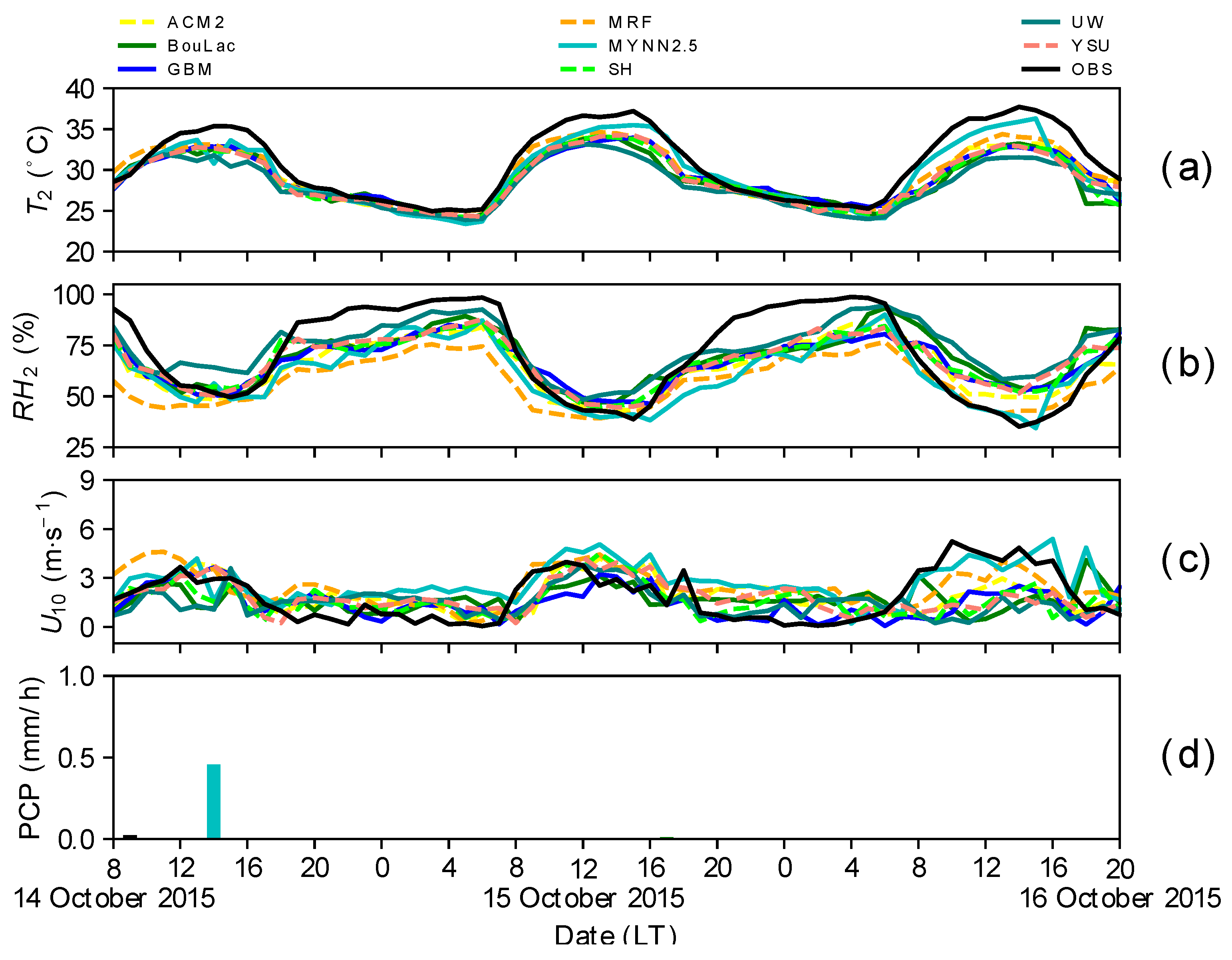
The predicted meteorological variables, such as T2, RH2, U10, and PCP for the 2014 dry period, are compared to observations (Figure 2). The observations show the typical diurnal pattern, with maximum temperatures during the afternoon and minimums near sunrise. The maximum T2 of 36.1 °C was recorded at 14 LT on 30 September, and a decreasing trend was noticed throughout the period (Figure 2a). In general, PBL schemes predict well for the first two days. Nonlocal PBL schemes tend to produce 1.0–2.0 °C warmer conditions in comparison to local PBL schemes.
All PBL schemes produced ≈ 5–15% drier conditions in comparison to observations (Figure 2b). Nonlocal (local) PBL schemes, such as MRF and ACM2 (BouLac and GBM), produce drier (wetter) conditions. Regarding the U10, all PBL schemes overestimated (0.5–1.5 m·s−1) the observations during the transition from afternoon to nighttime (Figure 2c). On the other hand, no PBL scheme was able to reproduce the increase observed during the morning transition stage (06–08 LT).
Two rainfall episodes (<5 mm·h−1) were captured by the instruments, one at 05 LT (2.3 mm·h−1) and other at 11 LT (3.6 mm·h−1) on 2 October (Figure 2d). These rainfalls induce air moistening, which decreases the temperature, leading to higher differences in comparison to predicted variables, since the model did not capture the observed rainfall. On the other hand, spurious rainfalls episodes were predicted. For instance, local GBM, UW, and MYNN2.5 schemes predicted rainfall episodes (<5.0 mm·h−1) on 1 October 2014, and UW and nonlocal YSU schemes predicted rain on 2 October, which was a higher amount (>10.0 mm·h−1) and delayed in time in comparison to observed ones. Both cooling and moistening, as well as strong winds (>5.0 m·s−1), were predicted during rainfall episodes, which may be associated with spurious (non-observed) rainfall predictions.

3.1.2. 2015 Dry Period

In contrast to the 2014 period, there is no rainfall during the selected dry period for 2015 (Figure 3). An increasing trend in temperature is noticed, with the maximum observed T2 being 37.7 °C at 14 LT on October 16 (Figure 3a). All PBL schemes predicted 1.3–2.7 °C colder temperatures. The local MYNN2.5 (UW) scheme predicted warmer (colder) conditions in comparison to other PBL schemes.
The nonlocal MRF (local MYNN2.5) scheme produced the driest conditions, mainly during the nighttime (daytime). Almost all PBL schemes present difficulties in reproducing the nighttime saturation. They do not completely depict the saturation, presenting 10–20% drier conditions in comparison to observations (Figure 3b).
A better agreement is seen in terms of U10 prediction between 06 and 08 LT in comparison to the 2014 period, particularly the local MYNN2.5 scheme, which shows a good agreement with the observed pattern. All PBL schemes presented a systematic overestimation of wind speed (0.5–1.5 m·s−1) at night when calm winds (<1.5 m·s−1) were observed mainly between 15 and 16 October (Figure 3c).
On the other hand, the PBL schemes underestimate (1.0–2.5 m·s−1) the observations during the daytime. Even though no precipitation was observed during the period (Figure 3d), the local MYNN2.5 scheme predicted 0.4 mm at 14 LT on 14 October.

3.2. Comparison of Predicted and Observed Surface Turbulent Fluxes

3.2.1. 2014 Dry Period

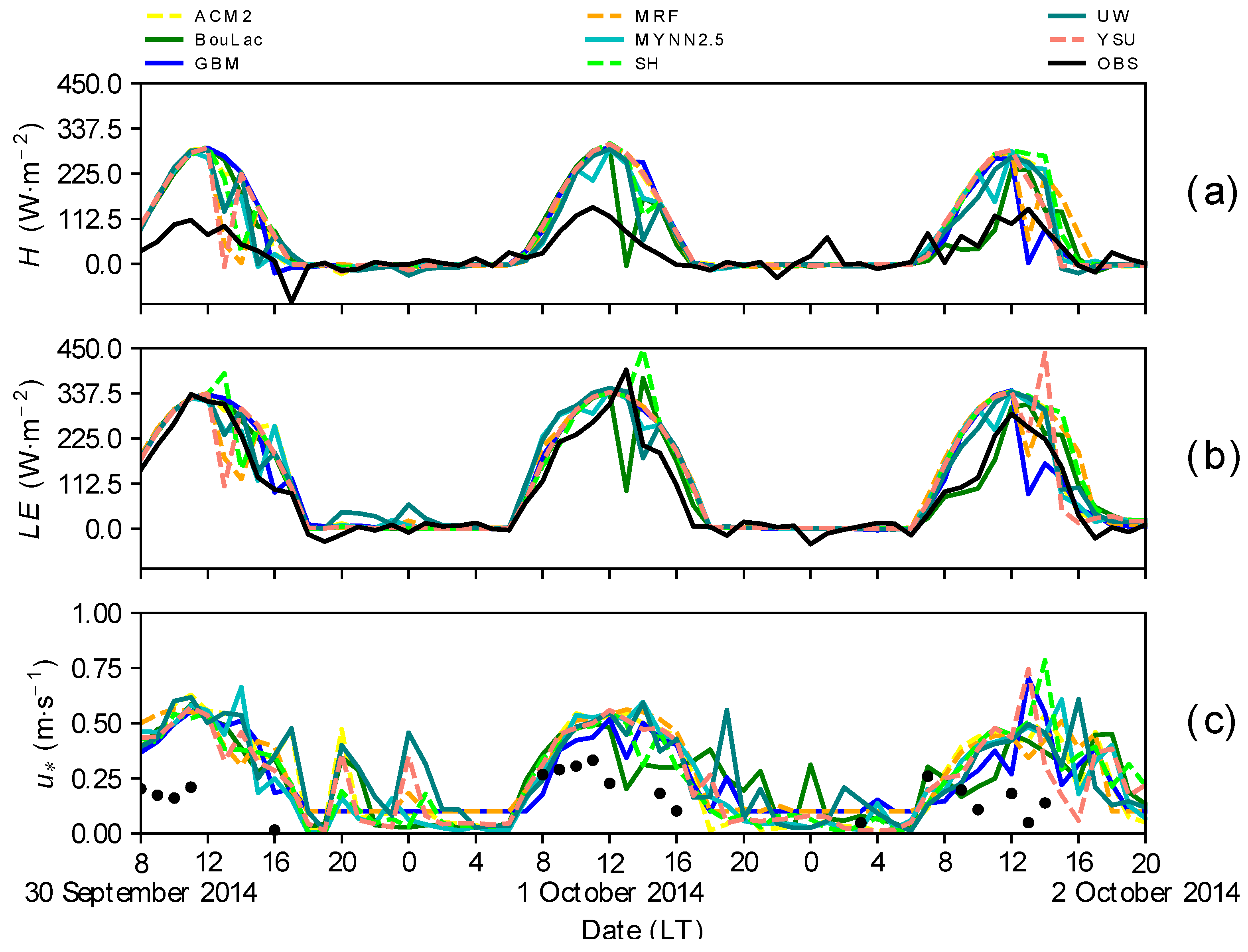
The predicted turbulent fluxes, such as H, LE, and u*, are compared to 30ECOR data [41] (Figure 4). The observed turbulent heat fluxes indicate that the available net radiation is predominantly transformed into LE during the daytime.
The observed H was about 60.0–140.0 W·m−2 between 09 and 13 LT (Figure 4a), with a maximum H of 141.0 W·m−2 occurring at 11 LT on 1 October. The comparison to predicted ones reveals that PBL schemes notably overestimate (>150%) the observations during daytime and slightly underestimate (up to 5.0 W·m−2) at night. Overall, the predictions are closer to each other, except during the afternoon, when some PBL schemes, for instance, YSU, BouLac, and GBM, present a sudden decrease near 14 LT.
Regarding LE (Figure 4b), a better agreement is seen among predictions and observations in comparison to H. The observed maximum LE was 396.0 W·m−2 at 13 LT on 1 October. The local BouLac scheme reproduces quite well the observations between sunrise and noon on 2 October, while all other PBL schemes overestimate the observations. A slight overestimation (up to 5.0 W·m−2) is seen at night. In general, the model setup was able to reliably reproduce the latent heat fluxes in comparison to sensible heat fluxes throughout the period.
Regarding the u* (Figure 4c), it presents some gaps related to measurement failures, especially at night. In the daytime, more data are available, revealing a systematic overestimation (0.25–0.50 m·s−1) that indicates excessive mechanical mixing produced by the PBL schemes between the morning and early afternoon.

3.2.2. 2015 Dry Period

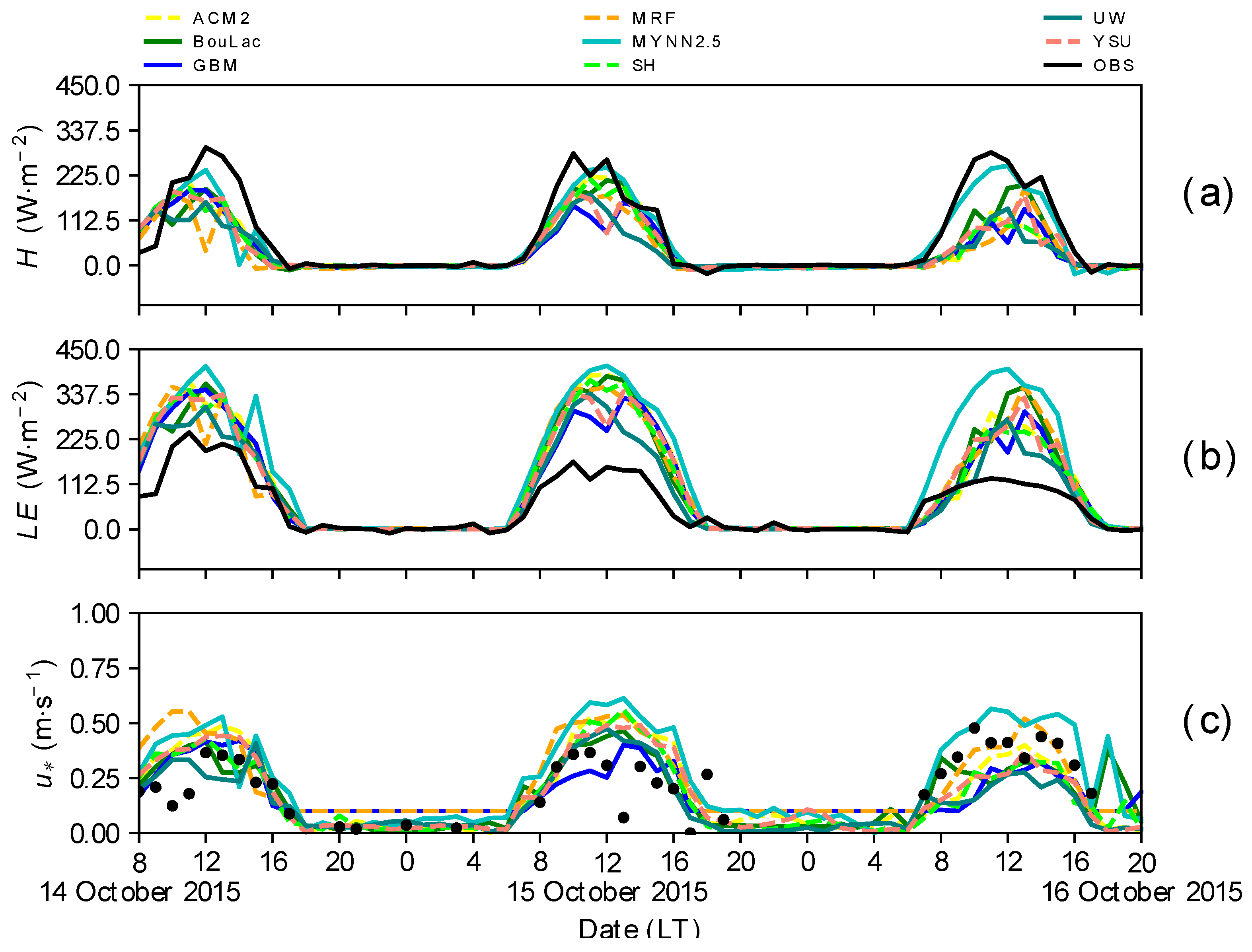
Unlike the 2014 dry period, the observed turbulent heat fluxes (Figure 5) reveal that the available net radiation is predominantly converted into H during the daytime. The average observed H is 74.0 W·m−2 with maximum values around 250.0 W·m−2 (Figure 5a), while the average LE is 60.0 W·m−2 with maximum values around 150.0 W·m−2 (Figure 5b). The differences are practically insignificant between the model and observation during nighttime for both turbulent heat fluxes in comparison to daytime.
The observed maximum H was 294.8 W·m−2 at 12 LT on 14 October, while the local MYNN2.5 scheme predicted 238.6 W·m−2, and the nonlocal MRF scheme predicted only 36.4 W·m−2. The local MYNN2.5 scheme presented the best agreement with the observations on 16 October, especially in the morning. All PBL schemes overestimate (>100%) the LE observations during daytime and present a delayed diurnal cycle in comparison to observation.
The observed maximum LE was 242.0 W·m−2 at 11 LT on 14 October, which all PBL schemes overestimate. In the following two days, a decreasing trend is seen in observations, with a maximum LE around 150.0 W·m−2. On the other hand, almost all PBL schemes predicted values higher than 350.0 W·m−2. Notably, the local MYNN2.5 scheme produces the highest turbulent heat flux amount in comparison to other PBL schemes.
Regarding u* (Figure 5c), more data are available in comparison to the 2014 period. In general, PBL schemes better predict the friction velocity, since that value agrees with observations during daytime. Local MYNN2.5 and nonlocal MRF schemes produced higher mechanical mixing in comparison to other PBL schemes. The observations during the daytime are closer to 0.5 m·s−1, while they are closer to 0.1 m·s−1 at night. Both local GBM and nonlocal MRF schemes overestimated (≈0.1 m·s−1) the observations in the early morning.

3.3. Comparison of Predicted and Observed PBL Structures

3.3.1. 2014 Dry Period

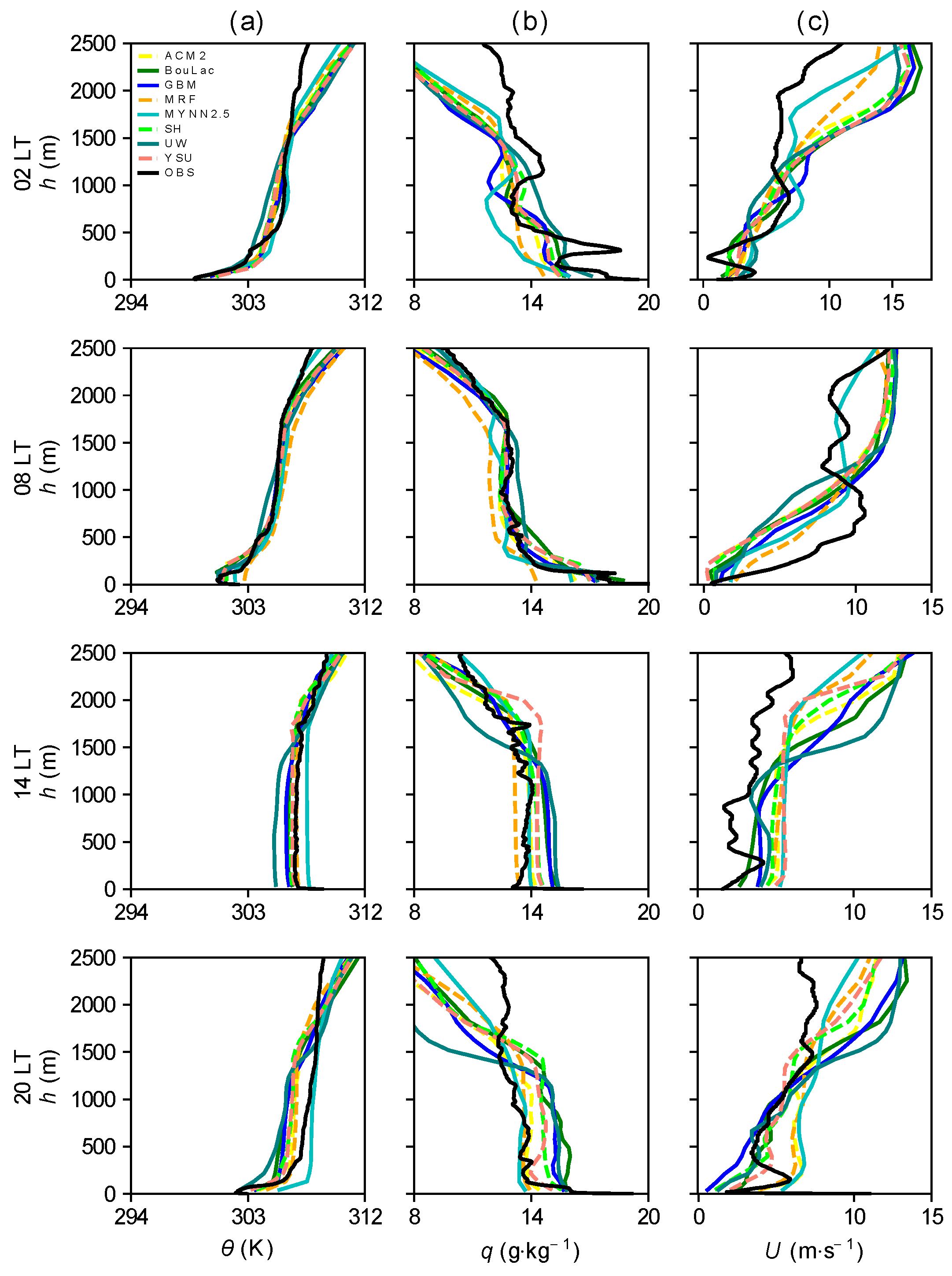
The predicted θ, q, and U profiles, corresponding to sounding measurements at 02, 08, 14, and 20 LT on 1 October 2014 (Figure 6), were chosen to represent a complete day, encompassing the day and nighttime patterns. For both study periods, we choice the second predicted day to comparison. In the nocturnal SBL stage at 02 LT, the observed θ profile (Figure 6a) increased by 7.0 K in the first 500 m from the ground. Most PBL schemes depicted the observed shape, even producing a 0.6 K colder bias near the surface, while producing 1.7 K warmer conditions above 1500 m. Almost all PBL schemes predicted 0.2–0.7 g·kg−1 wetter conditions in the first 1000 m from the ground and 1.0–2.3 g·kg−1 drier conditions above 1000 m (Figure 6b). The observed U profile during nocturnal SBL (Figure 6c) exhibits a typical jet shape near 550 m with 9.0 m·s−1. No PBL scheme reproduces the shape of the observed profile, which underestimates (2.0–3.5 m·s−1) the observations close to the surface and overestimates (1.0–3.0 m·s−1) above 1100 m.
All PBL schemes predicted 0.3–1.3 K warmer conditions in the first 2500 m at 08 LT, with the MYNN2.5 scheme being slightly warmer than other PBL schemes. Almost all PBL schemes predicted 0.1–1.2 g·kg−1 wetter conditions in the first 1000 m. Nonlocal ACM2, MRF, and YSU schemes presented 0.5–1.5 g·kg−1 drier bias closest to the surface. All PBL schemes predicted 0.5–3.5 g·kg−1 drier conditions above 1000 m. The wind jet pattern evolved during the early morning, producing a strong sheared wind speed profile where a vigorous jet is observed near 390 m with 13.0 m·s−1. Once again, no PBL scheme reproduced the observed shear and produced a flatter wind speed profile, underestimating the core of the jet wind speed by about 4.0–5.0 m·s−1. The differences diminish up to 1500 m height, with PBL schemes overestimating the observed wind speed by about 0.5–2.0 m·s−1.
An unstable θ profile is observed at 14 LT with 305.7 K on average within PBL, when the profiles predicted from PBL schemes exhibit different characteristics of stability (e.g., local PBL schemes behave stable near the surface, and nonlocal PBL schemes behave unstable). For instance, both nonlocal MRF and YSU schemes produce deeper mixing (unstable profile) throughout the PBL. The nonlocal SH scheme profile shows good agreement with the observed one. In general, all PBL schemes produced 0.1–2.0 K warmer conditions within the PBL in comparison to the observed profile. The observed q profile exhibits 15.4 g·kg−1 on average within PBL. All PBL schemes predicted 0.4–3.0 g·kg−1 drier conditions in the first 1500 m, especially the nonlocal ACM2, MRF, and YSU schemes. On the other hand, the predicted wetter conditions (0.6–1.0 g·kg−1) above the PBL indicate that these schemes produce excessive vertical mixing. The scale-aware mixing approach of the SH scheme produced a better agreement (0.2 g·kg−1 wetter) with the observed profile in comparison to the other nonlocal schemes, while the local MYNN2.5 and UW schemes produced the best agreement (0.1 g·kg−1 wetter). In comparison to early morning and morning, the differences between the observed U profile and the predicted ones at 14 LT are minor. Both the local UW and MYNN2.5 schemes tend to overestimate (2.5–4.0 m·s−1) the observations near the surface.
The major differences in comparison to observations during the night at 20 LT are near the surface (1.0–4.5 K colder) and above 1700 m (1.5–2.7 K colder). The nonlocal MRF scheme produced 0.5 K warmer conditions within the residual layer (region directly above the SBL, between around 250–1500 m). The local UW scheme shows a 2.6 K colder and more stable profile in comparison to the observed one. In general, the main differences in θ profiles are near the surface due to the stability predicted by the PBL schemes, which differ from the observed one, as well as above the SBL, which is related to misrepresentation of the residual layer. The differences among PBL schemes are notable in terms of q profiles. For instance, the local BouLac scheme produces the driest conditions (3.0 g·kg−1 on average in the first 1700 m and 6.0 g·kg−1 compared to observation at 750 m) in comparison to other PBL schemes, which all produced 0.4–3.0 g·kg−1 drier conditions in the first 1700 m. In contrast, all PBL schemes produced 0.7–2.9 g·kg−1 wetter conditions in comparison to observations above 1700 m. The predicted U profile at 20 LT lies on the observed sounding and roughly captures the shape, except the local BouLac scheme that overestimates (≈5.0 m·s−1) the observation with wind speeds higher than 10.0 m·s−1 near 1500 m.

3.3.2. 2015 Dry Period

The sounding measurements at 02, 08, 14, and 20 LT on 15 October 2015 were chosen for comparison to predicted ones. The observed θ profile at 02 LT (Figure 7a) exhibits an increase of 4.0 K on potential temperature until the top of the nocturnal SBL around 280 m. The observed profile reveals information above the SBL, as well as the presence of the residual layer from the previous day. The predicted θ profiles also show this pattern, with the local UW scheme presenting a good agreement (0.2 K colder) near the surface, while other PBL schemes present 0.3–0.9 K warmer conditions. Most PBL schemes tend to be 0.1–0.8 K colder within the residual layer except the local MYNN2.5 scheme (0.3 K warmer), and, above 1500 m, they all behave 0.7–1.5 K warmer. This may indicate that the observed residual layer is deeper in comparison to the predicted ones. Even though PBL schemes reproduced the drying until 170 m observed in the q profile (Figure 7b), they were unable to predict the 3.0 g·kg−1 moistening seen between 170 and 310 m. The local MYNN2.5 (UW) scheme produced both warmer (colder) and drier (wetter) conditions in the first 1000 m height. A low-level jet is observed on the U profile, with a sharper jet core reaching 4.0 m·s−1 of maximum speed at 80 m (Figure 7c). In general, the PBL schemes do not reproduce this pattern. On the other hand, the wind speed increases with height, reaching more than 15.0 m·s−1 near 2000 m, which was not observed (overestimation of around 10.0 m·s−1 at 2000 m).
The PBL schemes were able to produce better thermodynamic profiles (θ and q) at 08 LT in comparison to the ones predicted at 02 LT. Notably, the nocturnal SBL is being eroded by the thermals from the ground (indicated by the cooling and drying near the surface). The increase in θ with height until 500 m in the observation remains practically constant until around 1700 m. Major differences between measured and predicted profiles are near the surface and above 1700 m. In general, the nonlocal MRF scheme predicted warmer (0.5 K on average) and drier (0.7 g·kg−1 on average) conditions, especially near the surface. Most PBL schemes captured the observed q profile with reasonable agreement. On the other hand, the observed U profile is misrepresented, being underestimated (2.2–4.6 m·s−1) below the 1000 m and overestimated (0.2–2.5 m·s−1) above. A strong shear is seen from the surface until ≈750 m reaching 10.0 m·s−1 with a subsequent reduction, while PBL schemes produce a typical wind shear profile until 2500 m, reaching ≈ 12.0 m·s−1.
The diurnal mixed-layer at 14 LT is well reproduced by practically all PBL schemes, where a vigorous deeper layer is observed with 306.7 K on average in the first 1750 m. Nonlocal schemes (ACM2, MRF, YSU, and SH) tend to produce a better agreement with the observed θ profile in comparison to local schemes. For instance, consider UW (1.5 K colder) and MYNN2.5 (1.0 K warmer), which present major differences within the PBL. This better performance of nonlocal schemes is related to the inclusion of a nonlocal term, which promotes the nonlocal mixing related to larger eddies. The differences between observation and prediction are higher for the q profile. Within PBL, the average of the observed q is 13.6 g·kg−1. Local MYNN2.5 schemes reproduced the vertical structure with good agreement in the first 1000 m, while other local schemes (BouLac, GBM, and UW) produced 1.0–2.0 g·kg−1 wetter conditions. Nonlocal schemes were closer to the observed profile, where major differences were produced by the MRF (≈1.0 g·kg−1 drier) and YSU schemes (≈1.0 g·kg−1 wetter). The local UW scheme produced the greatest overall difference, being the driest condition (1.0 g·kg−1 on average) in the inversion layer. A typical convective boundary layer wind speed profile was predicted by all nonlocal schemes and local MYNN2.5, while local BouLac, GBM, and UW schemes showed significant differences from the observed U profile. In general, all PBL schemes overestimate (2.1–3.0 m·s−1) the observed U profile.
The comparison of observed and predicted profiles at 20 LT confirms that daytime profiles (08 and 14 LT) are in general better reproduced than nighttime ones. Meanwhile, the observed θ profile exhibits a stable stability close to the surface and a neutral stability above 1500 m, while most PBL schemes produce a neutral stability between 400 and 1500 m. This may be related to the differences in positioning of the daytime residual layer between observations and predictions. Local MYNN2.5 produces about 2.0 K warmer conditions near-surface, which is coherent with warmer daytime patterns, while the UW scheme is the colder one (about 1.5 K). Regarding q profiles, the differences are minor for local MYNN2.5 and nonlocal MRF, ACM2, and YSU schemes near the surface, while the other PBL schemes produced 1.5–1.9 g·kg−1 wetter conditions. Even though MYNN2.5, ACM2, and MRF schemes produced good agreement with the observed q profile, they poorly represented the observed U profile. A low-level jet can be seen at the bottom of the U profile (max. U of 6.0 m·s−1 at 150 m), whose PBL schemes are not able to be captured in predictions. The upper part of the predicted residual layer (above 1500 m) is, in general, 0.2–2.5 K warmer, 1.2–4.6 g·kg−1 drier, and has strong winds (>10.0 m·s−1) in comparison to observations.

3.4. Comparison of Predicted and Observed PBL Heights

As described earlier (see Section 2.3), a different method of PBL height calculation is used in each PBL scheme, which generates a broad variability among them even under the same atmospheric conditions. In general, local PBL schemes assume the PBLH as the level where the prognostic TKE falls into a threshold value, whereas, in the nonlocal PBL schemes, the PBLH computation is based on the Richardson number (Ri) with a dependency on temperature and wind speed profiles. Recap that some local PBL schemes, such as GBM and UW, also compute the PBLH based on the Ri number method. Furthermore, the PBLH is a fundamental variable, especially for nonlocal PBL schemes, since it is used to compute diffusion coefficients and counter-gradient terms. In this section, we evaluate the PBLH computed from each PBL scheme (default output). We do not use any external method to estimate PBL depth from predicted profiles. Each PBL scheme’s predicted PBLHs are validated against the ceilometer-estimated PBLH [43] (OBSCEIL, black line).

3.4.1. Diurnal Variations of PBL Height

2014 Dry Period

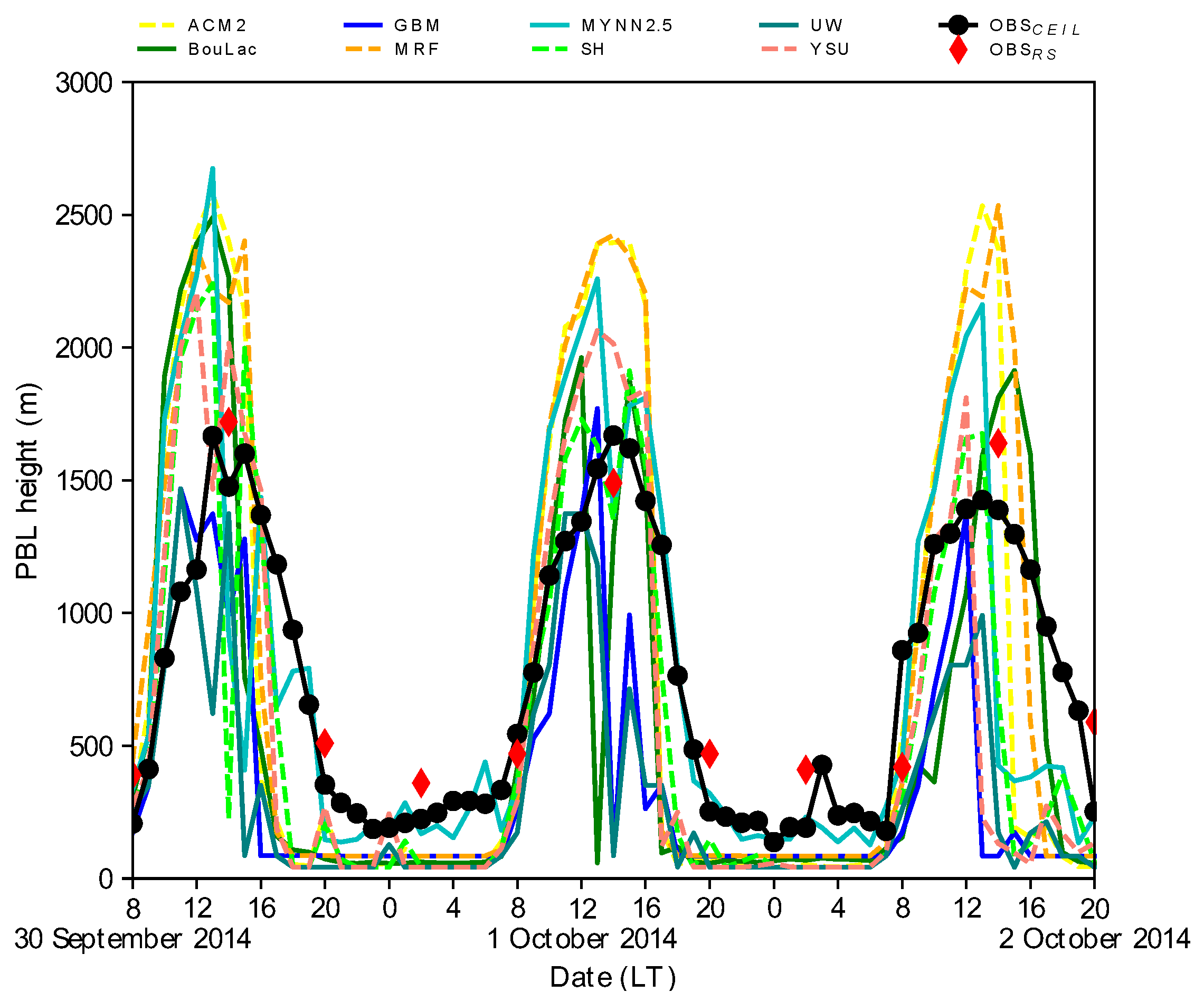
The observed PBLH in the 2014 studied dry period exhibits a decreasing trend, with heights near 1500 m during daytime (Figure 8). This decreasing pattern in observed in P B L H , which corroborates with the decreasing air temperature and increasing moisture along the period (Figure 2a,b). The erosion of nocturnal PBL starts at sunrise (06 LT), when the PBL begins to deepen [37]. Most PBL schemes start the PBL growth at sunrise in agreement with the observed pattern. The maximum PBLH of 1669 m was observed at 14 LT on 1 October 2014, when the average growth rate was 173 m·h−1, with a maximum rate of 231 m·h−1 between 08 and 09 LT achieved after the total erosion of nocturnal PBL. In general, most PBL schemes underestimate (99–536 m) the daytime PBL (06–18 LT). Only nonlocal ACM2 (MB = 175 m), MRF (MB = 228 m), and local MYNN2.5 (MB = 100 m) schemes overestimated the observations. Nonlocal MRF and ACM2 schemes predicted a deeper PBL, which is related to the warmer and drier conditions within the PBL at 14 LT (Figure 6a,b 14 LT). Note that the nonlocal YSU scheme adopts explicit entrainment in the top of PBL, which produces a lower PBL in comparison with the MRF and ACM2 schemes, resulting in better agreement with the observations near the inversion layer (Figure 6a 14 LT).
The shallower PBL, predicted by the local GBM (MB = −536 m) and UW (MB = −576 m) schemes, may be related to the PBLH method of definition, which, due to tiny gradients related to excessive mixing, leads to Rib exceeding the threshold in lower levels, generating systematically lower PBLHs [63]. The overestimation of observed PBLH may be also related to both excessive thermal and mechanical mixing (Figure 4), mainly in terms of sensible heat flux (Figure 4a). This may explain the predicted premature decaying of PBL by PBL schemes, seen during the afternoon.
Regarding the nighttime, the observed PBL was stable, with an average height of 287 m. All PBL schemes underestimated (57–232 m) the observations at night (19–05 LT), with the local MYNN2.5 scheme (MB = −57 m) presenting a smaller difference. The local UW scheme produces a shallower PBL (MB = −232 m) at night, with an average height of 50 m. The unrealistically lower PBLHs at night might be associated with the premature decay of PBL during the afternoon. The excessive mechanical mixing (noticed in Figure 4c) could help to explain the lower PBLHs, for instance, obtained using both local UW and GBM schemes. In terms of local PBL schemes with definition methods purely based on TKE, note that the BouLac scheme prescribes a larger TKE threshold (e = 0.005 m·s−2) in comparison to the MYNN2.5 scheme (e = 0.0001 m·s−1), which explains the lower PBLHs of the BouLac scheme (MB = −219 m) due to pronounced mixing activity near the surface and consequently reaching a higher TKE value in lower levels.

2015 Dry Period

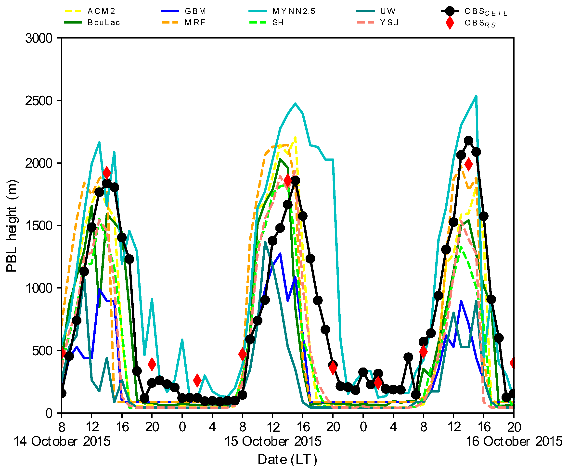
The observed PBLHs during the 2015 dry period are higher, and an increasing trend is observed (Figure 9) in comparison to the 2014 study period. This corroborates with higher temperatures and drying observed during the daytime (Figure 3a,b) as well as higher thermal mixing, especially due to a pronounced sensible heat flux (Figure 5a). The maximum PBLH of 2180 m was observed at 14 LT on 16 October 2015, with an average growth rate of 290 m·h−1 and a maximum rate of 536 m·h−1 between 12 and 13 LT. The deepest daytime PBLHs are predicted by the local MYNN2.5 scheme (MB = 362 m), with values higher than 2000 m. As noticed on 14 October, most PBL schemes tend to anticipate the PBL development, and, consequently, they anticipate the PBL decaying during the afternoon, leading to an overall underestimation (104–732 m) of the daytime PBL. Both GBM (MB = −644 m) and UW (MB = −732 m) schemes produce the shallowest PBLs, which may be related to their predicted colder and wetter conditions (Figure 3a,b).
On the other hand, the MYNN2.5 scheme maintained the turbulence for longer during the afternoon, which generated an unrealistically deeper PBL through the evening, certainly associated with pronounced turbulent fluxes. 16 October may be considered the best predicted day in comparison to previous days, since PBL schemes were able to reproduce the observed diurnal cycle with a better agreement despite differences in magnitude (either overestimating or underestimating).
The average observed PBLH between October 14 (evening) and 15 (early morning) was 150 m. A very stable PBL was observed between 00 and 06 LT, when most PBL schemes captured the observations, showing a shallower PBL probably related to the good agreement with the observed friction velocity. In this case, the local MYNN2.5 scheme performed poorly, since it predicted a higher nocturnal PBL and exhibits fluctuations. The scenario changes between 15 and 16 October, where a nocturnal PBL with weakly stable behavior is observed through PBLH measurements with an average height of 280 m. In general, almost all PBL schemes underestimated (130–173 m) the observations during the nighttime, except the local MYNN2.5 scheme, which overestimates them (MB = 191 m). Despite the overestimation, the scheme produced good agreement between October (evening) 15 and 16 (early morning). Local UW (MB = −173 m) and nonlocal SH (MB = −170 m) and YSU (MB = −169 m) schemes produced shallower PBLs at night.

3.5. Performance Analysis

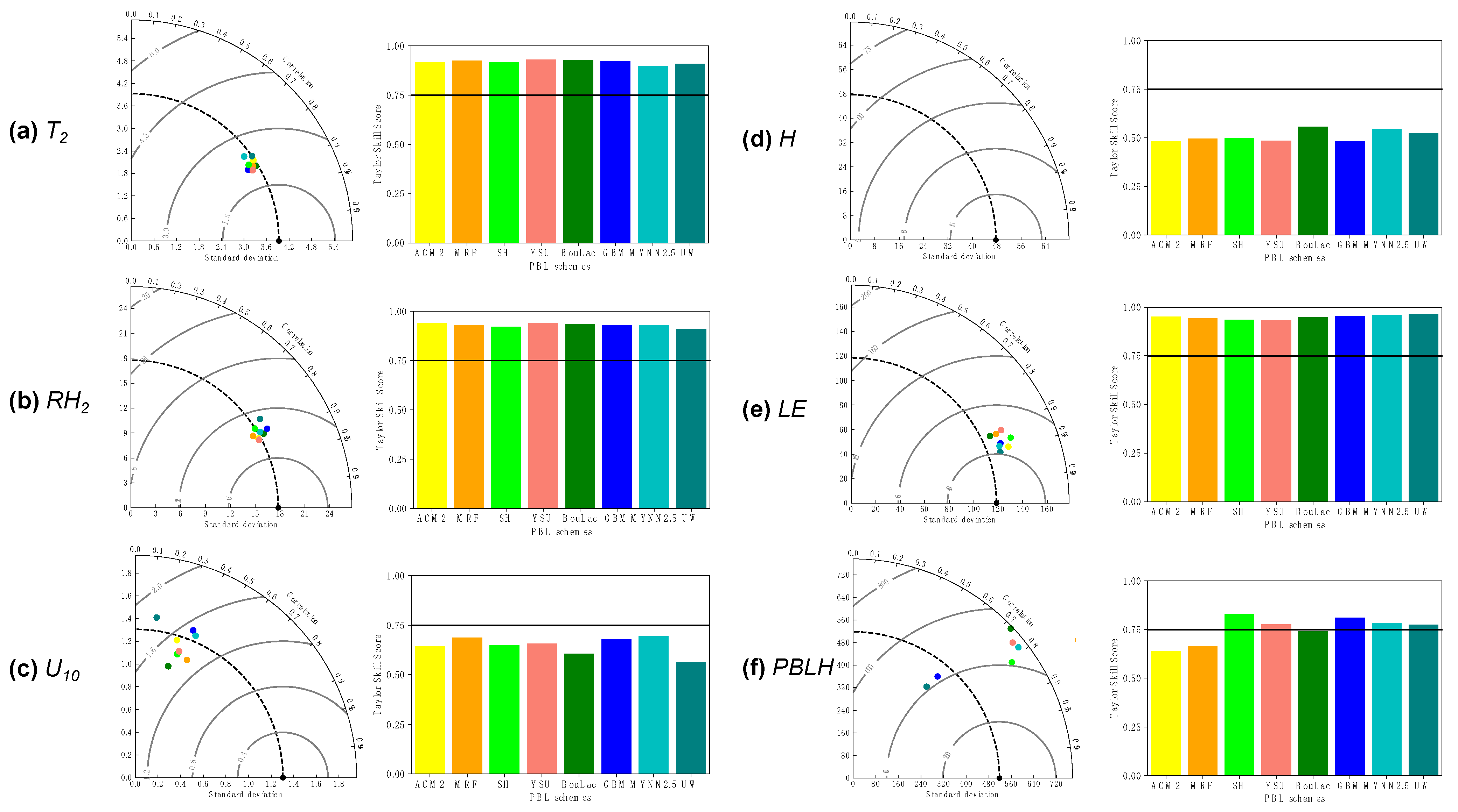
Figure 10 presents the Taylor diagrams (left) and Taylor skill score charts (right) for evaluated variables during the 2014 study period. PBL schemes presented a similar performance to predict T2 observations (Figure 10a), and the nonlocal YSU scheme (σ = 3.74 °C, CRMSE = 1.8 °C, r = 0.86, TSS = 0.93) performed better, while the local MYNN2.5 scheme presented a slightly worse performance (σ = 3.75 °C, CRMSE = 2.25 °C, r = 0.79, TSS = 0.90). The nonlocal MRF scheme produced the highest T2 overestimation (MB = 0.9 °C, Figure A1a T2 in Appendix A).
Evaluated PBL schemes also presented similar performance among them to predict observed RH2 (Figure 10b), with the nonlocal YSU scheme presenting the best performance (σ = 17.48%, CRMSE = 8%, r = 0.88, TSS = 0.94) and the local UW scheme the worst one (σ = 18.89%, CRMSE = 11%, r = 0.82, TSS = 0.91). Once again, nonlocal MRF scheme produced the higher underestimation and error (MB = −17%, RMSE = 20%, Figure A1a–c RH2).
Regarding U10 (Figure 10c), PBL schemes produced different performances among them, wherein the nonlocal MRF scheme produced the best performance (σ = 1.13 m·s−1, CRMSE = 1.3 m·s−1, r = 0.40, TSS = 0.69), and the local UW scheme produced the worst performance (σ = 1.42 m·s−1, CRMSE = 1.8 m·s−1, r = 0.13, TSS = 0.56), which is related to its higher overestimation and error (MB = 1.0 m·s−1, RMSE = 2.0 m·s−1, Figure A1a–c U10).
All PBL schemes produced in general the poorest performance to predict the observed H (Figure 10d) in comparison to the other variables, which is related to overestimation (MB > 35 W·m−2) and high error (RMSE > 70.0 W·m−2, Figure A1c), especially during daytime (see Figure 4a). The points relative to PBL schemes are not seen in the Taylor diagram due to the higher σ and CRMSE (twice as much than reference data). Nevertheless, the local BouLac scheme (σ = 97.6 W·m−2, CRMSE = 52.0 W·m−2, r = 0.78, TSS = 0.56) produced the best performance among PBL schemes (Figure 10e), certainly related to its lower overestimation (MB = 35.1 W·m−2, Figure A1a H).
In terms of PBLH prediction, PBL schemes captured the temporal variability of observed PBLH with different performances (Figure 10f). Only nonlocal ACM2 (MB = 6 m) and MRF (MB = 46 m), as well as local MYNN2.5 (MB = 33 m) schemes, overestimated the observed PBLH (Figure A1a PBLH). Both local GBM (MB = −393 m) and UW (MB = −430 m) schemes presented higher underestimations. Nonlocal SH scheme may be considered to have the best performance (σ = 695 m, CRMSE = 405.0 m, r = 0.81, TSS = 0.83), while the ACM2 scheme was the worst one (σ = 956 m, CRMSE = 550.0 m, r = 0.82, TSS = 0.64). This is related to the lower error produced by the SH scheme (RMSE = 443 m), as well as a higher error by ACM2 scheme (RMSE = 606 m, Figure A1c PBLH). Note that, according to the TSS chart, the SH, YSU, GBM, MYNN2.5, and UW schemes produced TSS higher than 0.75. Figure 11a shows the computed TSS separately for daytime and nighttime PBLH for the 2014 study period, revealing that, although SH, GBM, and UW schemes performed slightly better than MYNN2.5 during daytime, only this scheme performed well to reproduce the nocturnal PBLH (TSS = 0.76), while all other PBL schemes presented a lower TSS (<0.50). Thus, the MYNN2.5 scheme might be assumed as the best option to predict PBLH, mainly at night.
The local MYNN2.5 scheme produced the overall best performance (σ closer to reference data, lower CRMSE, and both r and TSS closer/higher than 0.75) to predict T2, RH2, U10, and H for the 2015 study period (Figure 12) in comparison to other PBL schemes. In general, most PBL schemes presented similar performance to predict T2 (Figure 12a) and RH2 (Figure 12b), with TSS being higher than 0.75 for T2, and TSS was higher than 0.60 for RH2. Almost all PBL schemes presented TSS below 0.75 to U10 (Figure 12c), and the local BouLac scheme produces the worst performance (σ = 0.74 m·s−1, CRMSE = 1.6 m·s−1, r = 0.09, TSS = 34). All PBL schemes underestimated (1.2–2.6 °C) the observations for T2, and almost all schemes underestimated (2–14%) the observations for RH2 (except UW scheme, MB = 2%), and only the ACM2 (MB = 0.1 m·s−1), MRF (MB = 0.6 m·s−1), and MYNN2.5 (MB = 0.8 m·s−1) schemes overestimated the observations for U10 (Figure A1b).
In contrast to the 2014 study period, PBL schemes performed better in the prediction of H (Figure 12d). On the other hand, the LE (Figure 12e) was the poorest predicted variable, which is associated with the overestimation (Figure A1b LE), especially during the daytime (see Figure 5b). The local UW scheme presented the least bad performance (TSS = 0.78) among PBL schemes to predict LE, which is related to its lower overestimation (MB = 31.9 W·m−2) and error (RMSE = 62.9 W·m−2, Figure A1b–d). The local MYNN2.5 scheme presented lower overestimation (MB = −12.2 W·m−2) and error (RMSE = 40.6 W·m−2) for H (Figure A1b–d H).
The PBL schemes produced spread performances in comparison to each other to predict the PBLH (Figure 12f). Only local GBM (MB = −425 m) and UW (MB = −494 m, Figure A1b PBLH) schemes presented TSS lower than 0.75, which is related to the prediction of unrealistically low PBLHs. Nonlocal ACM2, SH, and YSU, as well as local BouLac and MYNN2.5 schemes, showed a similar performance in terms of TSS (>0.87). In particular, the local MYNN2.5 scheme may be assumed to have the best overall performance (σ = 848 m, CRMSE = 430 m, r = 0.86, TSS = 0.87) for PBLH prediction, especially according to Figure 11b, which shows the scheme as having the best performance during both the daytime (TSS = 0.87) and the nighttime PBLH (TSS = 0.19). In comparison to the 2014 study period, the MYNN2.5 scheme showed a lower performance to predict nocturnal PBLH, probably associated to the overestimation seen between October 14 (evening) and 15 (early morning).

4. Conclusions

The performances of eight PBL schemes (ACM2, BouLac, GBM, MRF, MYNN2.5, SH, UW, and YSU) were evaluated on WRF model forecasts over the central Amazon basin during dry conditions, taking advantage of detailed observations from GoAmazon2014/5 field campaign datasets for model validation. It is important to point out that the presented performances of PBL schemes are a combination of three-day dry periods (2014—typical year and 2015—ENSO influenced year), the accuracy of initial conditions from NCEP-GFS forecast data, and errors in the 1-km resolution WRF numerical experiments.
Overall, the results revealed that nonlocal PBL schemes overestimated (0.1–0.9 °C) observations for T2 on 2014 study period, while mostly local PBL schemes underestimated (0.1–0.2 °C), which may be associated to the predicted rainfall out of phase with the observations. On the other hand, all PBL schemes underestimate T2 observations (1.2–2.6 °C) on the 2015 study period. In terms of RH2, almost all PBL schemes produced drier conditions (6–17% 2014, 2–14% 2015) on both studied periods. All PBL schemes overestimated (0.5–1.0 m·s−1) observations for U10 on 2014, whereas nonlocal PBL schemes presented equal bias (0.7 m·s−1). For the 2015 study period, most PBL schemes produced a negative bias (0.1–0.4 m·s−1). In general, among meteorological variables, the PBL schemes perform best for T2, which is a behavior already known [28,31]. Nonlocal PBL schemes performed better on the prediction of meteorological variables (YSU for both T2 and RH2, and MRF for U10) for the 2014 study period, while the local MYNN2.5 scheme produced the overall best performance for the 2015 study period.
A systematic overestimation (>100%) of either sensible or latent heat fluxes is noticed, especially during daytime, which corroborates with previous studies [31,63]. Turbulent heat fluxes were overestimated (35.1–51.4 W·m−2) in the 2014 studied period by all PBL schemes being related to the predicted spurious rainfall and consequently differences in cloud cover (discussed in terms of incoming radiation using SEBS data [64] presented throughout Figures S1 and S2 on Supplementary Material), on the other hand, the pronounced H observed in the 2015 study period was underestimated (25.6–38.9 W·m−2). The larger LE (smaller H) produced in the 2015 study period by the model may be associated with energy partitioning in the surface layer, as well as the land-use category due to the presence of areas with higher surface moisture (i.e., surrounding forest near the T3 site) [65]. Despite gaps in the friction velocity measurements, the comparison reveals that all PBL schemes overestimate the observations from the 2014 study period, which indicates excessive mechanical mixing. For the 2015 study period, a better agreement is seen, and, in particular, both nonlocal MRF and local GBM schemes produce higher u* at night. The overestimation of the friction velocity on the WRF model can be attributed to the drying of the lower PBL as a result of deep vertical mixing [66], as noted in the thermodynamic profiles. For instance, the PBL schemes produced a better agreement for friction velocity measurements over the 2015 period, which is associated with the better agreement between observed and modeled profiles.
Thermodynamic vertical structures are better reproduced in comparison to wind speed profiles. The daytime profiles (08 and 14 LT) are better reproduced than the nighttime (20 and 02 LT) ones, probably due to inconsistencies in the stability regime predicted by the PBL schemes in comparison to the observed, as well as the misrepresentation of the residual layer present above the SBL on nocturnal profiles. Nonlocal PBL schemes presented a warmer and drier bias on daytime mixed-layer profiles (14 LT), while local PBL schemes are closer to observations, even presenting different stability characteristics near the surface, with consequences on the reproduction of the observed θ profile at night (20 LT). In the case of the deeper mixed-layer observed in the 2015 study period, nonlocal PBL schemes presented quite good agreement, while local PBL schemes presented either colder or warmer, and in general, wetter biases.
Most PBL schemes present difficulty reproducing the nocturnal PBLH that is, in general, underestimated, which corroborates with previous studies [31]. This may be associated with the out-of-phase PBL development. The PBL schemes tend to rapidly deepen the PBL during the morning leading to overestimation, and, consequently, the PBL decaying is anticipated. In some cases, the development is maintained for longer, and the PBL decaying is delayed. The local MYNN2.5 scheme produces the best performance for predicting nocturnal PBLH in comparison to other PBL schemes. Nonlocal ACM2 and MRF (local MYNN2.5) schemes produced deeper PBL during daytime in the 2014 (2015) study period, while both GBM and UW schemes produced, in general, unrealistically lower PBLHs with the 1-km grid resolution. In general, the local MYNN2.5 scheme presented the best performance for PBLH prediction in both study periods.

Supplementary Materials

The following supporting information can be downloaded at: https://www.mdpi.com/article/10.3390/atmos14050850/s1, Figure S1: (a) Comparison of models predicted (eight PBL schemes) and SEBS observations [66] for downward longwave incoming radiation (W·m−2) and (b) downward shortwave incoming radiation (W·m−2) from 30 September to 2 October 2014, starting at 08 LT (X-axis is date and local time). Results from local (nonlocal) PBL schemes are plotted with filled (dashed) lines; Figure S2: Same as for Figure S1, but for the period from 14 to 16 October 2015.

Author Contributions

Conceptualization, J.A.M.J., G.F. and J.A.A.; methodology, J.A.M.J., J.A.A. and G.F.; software, J.A.M.J. and J.A.A.; validation, J.A.M.J. and R.G.C.; formal analysis, J.A.M.J., J.A.A. and G.F.; investigation, J.A.M.J., J.A.A. and G.F.; resources, J.A.M.J., J.A.A. and G.F.; data curation, J.A.M.J. and R.G.C.; writing—original draft preparation, J.A.M.J.; writing—review and editing, J.A.M.J., J.A.A., G.F. and R.G.C.; visualization, J.A.M.J.; supervision, J.A.A. and G.F.; project administration, J.A.A. and G.F.; funding acquisition, G.F. All authors have read and agreed to the published version of the manuscript.

Funding

This research was funded in part by the Coordenação de Aperfeiçoamento de Pessoal de Nível Superior-Brasil (CAPES)—Finance Code 001 and the Conselho Nacional de Desenvolvimento Tecnológico (CNPq). José Antonio Mantovani Júnior acknowledges CNPq for his grant (GM/GD 131094/2020-3). Gilberto Fisch acknowledges CNPq for his grant (PQ 307048/2018-7). Rayonil Carneiro acknowledges CNPq for his grant (process number 151920/2022-2).

Institutional Review Board Statement

Not applicable.

Informed Consent Statement

Not applicable.

Data Availability Statement

Data are available upon request from the authors.

Acknowledgments

We thank the GoAmazon2014/5 field campaign team for their efforts in producing and maintaining the datasets employed in the present study. This work was undertaken on the Santos Dumont supercomputer, part of the SINAPAD (Sistema Nacional de Processamento de Alto Desempenho) high-performance computing resources from Laboratório Nacional de Computação Científica (LNCC) located at Petrópolis, Rio de Janeiro, Brazil.

Conflicts of Interest

The authors declare no conflict of interest.

Appendix A

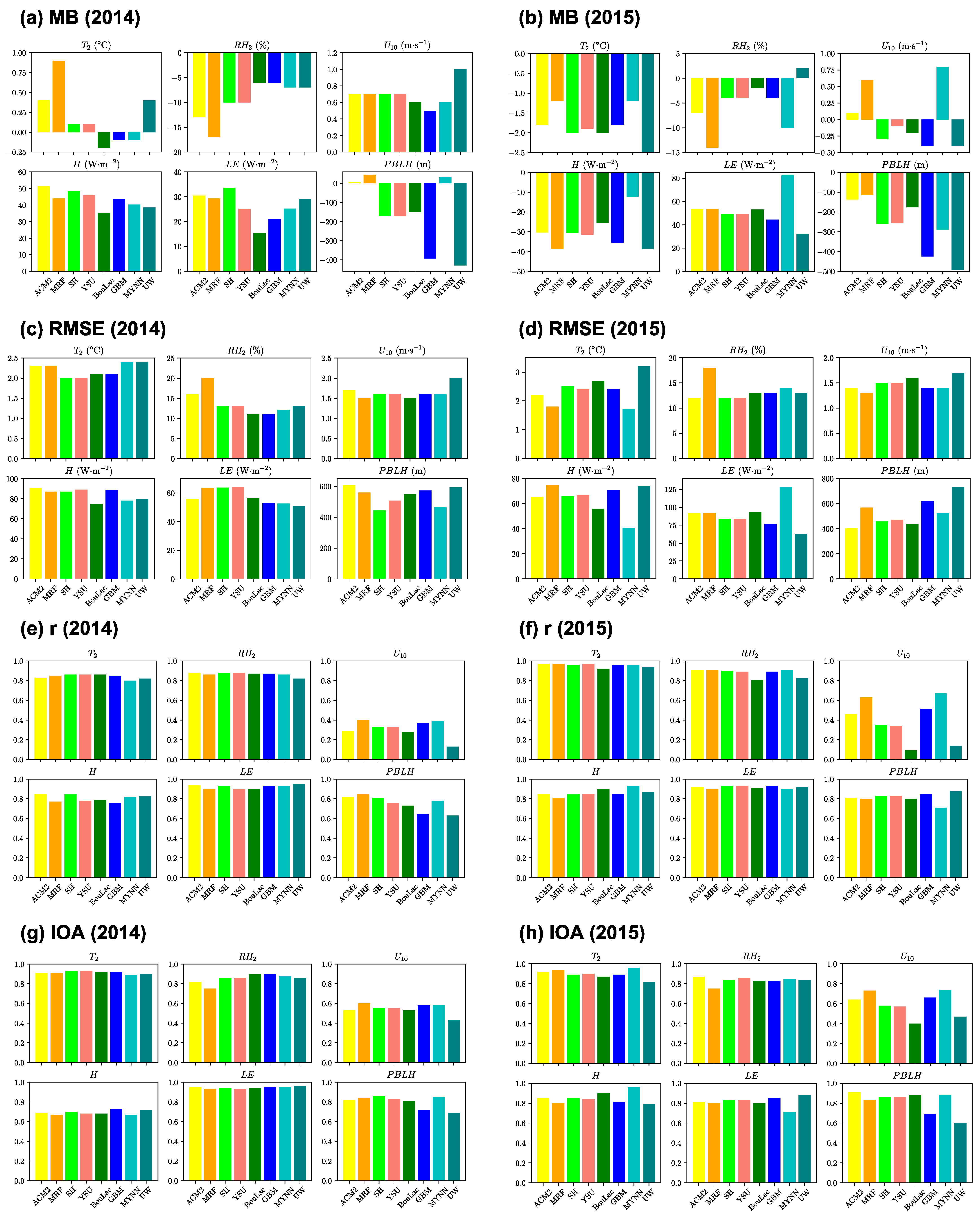
Figure A1 presents the statistical metrics computed for both studied periods (2014 and 2015) using GoAmazon2014/5 datasets [40,41,42,43] as reference data.
Figure A1. Statistical indexes computed for T2, RH2, U10, H, LE, and PBLH relative to each PBL scheme over the entire 2014 and 2015 periods, respectively. (a,b) Mean bias (MB), (c,d) root-mean-square-error (RMSE), (e,f) correlation coefficient (r), and (g,h) index of agreement (IOA).
Atmosphere 14 00850 g0a1

References

  1. Soares, P.M.M.; Miranda, P.M.A.; Siebesma, A.P.; Teixeira, J. An eddy-diffusivity/mass-flux parametrization for dry and shallow cumulus convection. Q. J. R. Meteorol. Soc. 2004, 130, 3365–3383. [Google Scholar] [CrossRef]
  2. Hu, X.-M.; Nielsen-Gammon, J.W.; Zhang, F. Evaluation of Three Planetary Boundary Layer Schemes in the WRF Model. J. Appl. Meteorol. Clim. 2010, 49, 1831–1844. [Google Scholar] [CrossRef]
  3. Zhang, X. Subgrid Turbulence Mixing. In Uncertainties in Numerical Weather Prediction, 1st ed.; Olafsson, H., Bao, J.-W., Eds.; Elsevier: Amsterdam, The Netherlands, 2021; pp. 205–227. [Google Scholar] [CrossRef]
  4. de Lange, A.; Naidoo, M.; Garland, R.M.; Dyson, L.L. Sensitivity of meteorological variables on planetary boundary layer parameterization schemes in the WRF-ARW model. Atmos. Res. 2020, 247, 105214. [Google Scholar] [CrossRef]
  5. Njuki, S.M.; Mannaerts, C.M.; Su, Z. Influence of Planetary Boundary Layer (PBL) Parameterizations in the Weather Research and Forecasting (WRF) Model on the Retrieval of Surface Meteorological Variables over the Kenyan Highlands. Atmosphere 2022, 13, 169. [Google Scholar] [CrossRef]
  6. de Lange, A.; Naidoo, M.; Garland, R.M.; Dyson, L.L. The sensitivity of simulated surface-level pollution concentrations to WRF-ARW-model PBL parameterisation schemes over the Highveld of South Africa. Atmos. Res. 2021, 254, 105517. [Google Scholar] [CrossRef]
  7. Yang, J.; Tang, Y.; Han, S.; Liu, J.; Yang, X.; Hao, J. Evaluation and improvement study of the Planetary Boundary-Layer schemes during a high PM2.5 episode in a core city of BTH region, China. Sci. Total Environ. 2020, 765, 142756. [Google Scholar] [CrossRef]
  8. He, J.; Chen, D.; Gu, Y.; Jia, H.; Zhong, K.; Kang, Y. Evaluation of planetary boundary layer schemes in WRF model for simulating sea-land breeze in Shanghai, China. Atmospheric Res. 2022, 278, 106337. [Google Scholar] [CrossRef]
  9. Louis, J.-F. A parametric model of vertical eddy fluxes in the atmosphere. Bound.-Layer Meteorol. 1979, 17, 187–202. [Google Scholar] [CrossRef]
  10. Mellor, G.L.; Yamada, T. Development of a turbulence closure model for geophysical fluid problems. Rev. Geophys. 1982, 20, 851–875. [Google Scholar] [CrossRef]
  11. Troen, I.B.; Mahrt, L. A simple model of the atmospheric boundary layer; sensitivity to surface evaporation. Bound.-Layer Meteorol. 1986, 37, 129–148. [Google Scholar] [CrossRef]
  12. Hong, S.Y.; Pan, H.L. Nonlocal boundary layer vertical diffusion in a medium-range forecast model. Mon. Weather Rev. 1996, 124, 2322–2339. [Google Scholar] [CrossRef]
  13. Sukoriansky, S.; Galperin, B.; Perov, V. Application of a New Spectral Theory of Stably Stratified Turbulence to the Atmospheric Boundary Layer over Sea Ice. Bound.-Layer Meteorol. 2005, 117, 231–257. [Google Scholar] [CrossRef]
  14. Pleim, J.E. A Combined Local and Nonlocal Closure Model for the Atmospheric Boundary Layer. Part I: Model Description and Testing. J. Appl. Meteorol. Climatol. 2007, 46, 1383–1395. [Google Scholar] [CrossRef]
  15. Angevine, W.M.; Jiang, H.; Mauritsen, T. Performance of an eddy diffusivity–mass flux scheme for shallow cumulus boundary layers. Mon. Weather Rev. 2010, 138, 2895–2912. [Google Scholar] [CrossRef]
  16. Shin, H.H.; Hong, S.-Y. Representation of the Subgrid-Scale Turbulent Transport in Convective Boundary Layers at Gray-Zone Resolutions. Mon. Weather Rev. 2015, 143, 250–271. [Google Scholar] [CrossRef]
  17. Zhang, C.; Wang, Y.; Xue, M. Evaluation of an E–ε and Three Other Boundary Layer Parameterization Schemes in the WRF Model over the Southeast Pacific and the Southern Great Plains. Mon. Weather Rev. 2020, 148, 1121–1145. [Google Scholar] [CrossRef]
  18. Cohen, A.E.; Cavallo, S.M.; Coniglio, M.C.; Brooks, H.E. A Review of Planetary Boundary Layer Parameterization Schemes and Their Sensitivity in Simulating Southeastern U.S. Cold Season Severe Weather Environments. Weather Forecast. 2015, 30, 591–612. [Google Scholar] [CrossRef]
  19. Shin, H.H.; Hong, S.-Y. Intercomparison of Planetary Boundary-Layer Parametrizations in the WRF Model for a Single Day from CASES-99. Bound.-Layer Meteorol. 2011, 139, 261–281. [Google Scholar] [CrossRef]
  20. Wang, W.; Shen, X.; Huang, W. A Comparison of Boundary-Layer Characteristics Simulated Using Different Parametrization Schemes. Bound.-Layer Meteorol. 2016, 161, 375–403. [Google Scholar] [CrossRef]
  21. Moya-Álvarez, A.S.; Estevan, R.; Kumar, S.; Rojas, J.L.F.; Ticse, J.J.; Martínez-Castro, D.; Silva, Y. Influence of PBL parameterization schemes in WRF_ARW model on short—Range precipitation’s forecasts in the complex orography of Peruvian Central Andes. Atmos. Res. 2020, 233, 104708. [Google Scholar] [CrossRef]
  22. Jo, H.-Y.; Lee, H.-J.; Jo, Y.-J.; Heo, G.; Lee, M.; Kim, J.-A.; Park, M.-S.; Lee, T.; Kim, S.-W.; Lee, Y.-H.; et al. A case study of heavy PM2.5 secondary formation by N2O5 nocturnal chemistry in Seoul, Korea in January 2018: Model performance and error analysis. Atmos. Res. 2021, 266, 105951. [Google Scholar] [CrossRef]
  23. Lee, H.-J.; Jo, H.-Y.; Kim, J.-M.; Bak, J.; Park, M.-S.; Kim, J.-K.; Jo, Y.-J.; Kim, C.-H. Nocturnal Boundary Layer Height Uncertainty in Particulate Matter Simulations during the KORUS-AQ Campaign. Remote Sens. 2023, 15, 300. [Google Scholar] [CrossRef]
  24. Tyagi, B.; Magliulo, V.; Finardi, S.; Gasbarra, D.; Carlucci, P.; Toscano, P.; Zaldei, A.; Riccio, A.; Calori, G.; D’allura, A.; et al. Performance Analysis of Planetary Boundary Layer Parameterization Schemes in WRF Modeling Set Up over Southern Italy. Atmosphere 2018, 9, 272. [Google Scholar] [CrossRef]
  25. Griffin, S.M.; Otkin, J.A. Evaluating the Impact of Planetary Boundary Layer, Land Surface Model, and Microphysics Parameterization Schemes on Simulated GOES-16 Water Vapor Brightness Temperatures. Atmosphere 2022, 13, 366. [Google Scholar] [CrossRef]
  26. Shen, W.; Lu, Z.; Ye, G.; Zhang, Y.; Chen, S.; Xu, J. Exploring the Impact of Planetary Boundary Layer Schemes on Rainfall Forecasts for Typhoon Mujigae, 2015. Atmosphere 2022, 13, 220. [Google Scholar] [CrossRef]
  27. Falasca, S.; Gandolfi, I.; Argentini, S.; Barnaba, F.; Casasanta, G.; Di Liberto, L.; Petenko, I.; Curci, G. Sensitivity of near-surface meteorology to PBL schemes in WRF simulations in a port-industrial area with complex terrain. Atmos. Res. 2021, 264, 105824. [Google Scholar] [CrossRef]
  28. Zhang, L.; Xin, J.; Yin, Y.; Chang, W.; Xue, M.; Jia, D.; Ma, Y. Understanding the Major Impact of Planetary Boundary Layer Schemes on Simulation of Vertical Wind Structure. Atmosphere 2021, 12, 777. [Google Scholar] [CrossRef]
  29. Jia, W.; Zhang, X. The role of the planetary boundary layer parameterization schemes on the meteorological and aerosol pollution simulations: A review. Atmos. Res. 2020, 239, 104890. [Google Scholar] [CrossRef]
  30. Wang, C.; Qian, Y.; Duan, Q.; Huang, M.; Berg, L.K.; Shin, H.H.; Feng, Z.; Yang, B.; Quan, J.; Hong, S.; et al. Assessing the sensitivity of land-atmosphere coupling strength to boundary and surface layer parameters in the WRF model over Amazon. Atmos. Res. 2019, 234, 104738. [Google Scholar] [CrossRef]
  31. Wang, C.; Qian, Y.; Duan, Q.; Huang, M.; Yang, Z.; Berg, L.K.; Gustafson, W.I.; Feng, Z.; Liu, J.; Quan, J. Quantifying physical parameterization uncertainties associated with land-atmosphere interactions in the WRF model over Amazon. Atmos. Res. 2021, 262, 105761. [Google Scholar] [CrossRef]
  32. Prein, A.F.; Ge, M.; Valle, A.R.; Wang, D.; Giangrande, S.E. Towards a Unified Setup to Simulate Mid-Latitude and Tropical Mesoscale Convective Systems at Kilometer-Scales. Earth Space Sci. 2022, 9, 8. [Google Scholar] [CrossRef]
  33. Martin, C.L.; Fitzjarrald, D.; Garstang, M.; Oliveira, A.P.; Greco, S.; Browell, E. Structure and growth of the mixing layer over the Amazonian rain forest. J. Geophys. Res. Atmos. 1988, 93, 1361–1375. [Google Scholar] [CrossRef]
  34. Betts, A.K.; Fisch, G.; Von Randow, C.; Silva Dias, M.A.F.; Cohen, J.C.P.; Da Silva, R.; Fitzjarrald, D.R. The Amazonian boundary layer and mesoscale circulations. Amazon. Glob. Chang. 2009, 186, 163–181. [Google Scholar] [CrossRef]
  35. Martin, S.T.; Artaxo, P.; Machado, L.A.T.; Manzi, A.O.; Souza, R.A.F.; Schumacher, C.; Wang, J.; Andreae, M.O.; Barbosa, H.M.J.; Fan, J.; et al. Introduction: Observations and Modeling of the Green Ocean Amazon (GoAmazon2014/5). Atmos. Meas. Tech. 2016, 16, 4785–4797. [Google Scholar] [CrossRef]
  36. Henkes, A.; Fisch, G.; Machado, L.A.T.; Chaboureau, J.-P. Morning boundary layer conditions for shallow to deep convective cloud evolution during the dry season in the central Amazon. Atmos. Meas. Tech. 2021, 21, 13207–13225. [Google Scholar] [CrossRef]
  37. Carneiro, R.G.; Fisch, G. Observational analysis of the daily cycle of the planetary boundary layer in the central Amazon during a non-El Niño year and El Niño year (GoAmazon project 2014/5). Atmos. Meas. Tech. 2020, 20, 5547–5558. [Google Scholar] [CrossRef]
  38. Carneiro, R.; Fisch, G.; Neves, T.; Santos, R.; Santos, C.; Borges, C. Nocturnal Boundary Layer Erosion Analysis in the Amazon Using Large-Eddy Simulation during GoAmazon Project 2014/5. Atmosphere 2021, 12, 240. [Google Scholar] [CrossRef]
  39. Mather, J.H.; Voyles, J.W. The Arm Climate Research Facility: A Review of Structure and Capabilities. Bull. Am. Meteorol. Soc. 2013, 94, 377–392. [Google Scholar] [CrossRef]
  40. Kyrouac, J.; Springston, S. Meteorological Measurements Associated with the Aerosol Observing System (AOSMET). 2014. Available online: https://adc.arm.gov/discovery/#/results/instrument_code::aosmet (accessed on 10 October 2021).
  41. Sullivan, R.; Billesbach, D.; Keeler, E.; Ermold, B. Eddy Correlation Flux Measurement System (30ECOR). 2014. Available online: https://adc.arm.gov/discovery/#/results/instrument_code::30ecor (accessed on 10 October 2021).
  42. Keeler, E.; Coulter, R.; Kyrouac, J. Balloon-Borne Sounding System (SONDEWNPN). 2014. Available online: https://adc.arm.gov/discovery/#/results/instrument_code::sondewnpn (accessed on 10 October 2021).
  43. Morris, V.; Briam. Boundary-Layer Height Data with CEIL (CEILPBLHT). 2014. Available online: https://adc.arm.gov/discovery/#/results/instrument_code::ceilpblht (accessed on 10 October 2021).
  44. Wiegner, M.; Madonna, F.; Binietoglou, I.; Forkel, R.; Gasteiger, J.; Geiß, A.; Pappalardo, G.; Schäfer, K.; Thomas, W. What is the benefit of ceilometers for aerosol remote sensing? An answer from EARLINET. Atmos. Meas. Tech. 2014, 7, 1979–1997. [Google Scholar] [CrossRef]
  45. Kotthaus, S.; O’Connor, E.; Münkel, C.; Charlton-Perez, C.; Haeffelin, M.; Gabey, A.M.; Grimmond, C.S.B. Recommendations for processing atmospheric attenuated backscatter profiles from Vaisala CL31 ceilometers. Atmos. Meas. Tech. 2016, 9, 3769–3791. [Google Scholar] [CrossRef]
  46. Geiß, A.; Wiegner, M.; Bonn, B.; Schäfer, K.; Forkel, R.; Von Schneidemesser, E.; Münkel, C.; Chan, K.L.; Nothard, R. Mixing layer height as an indicator for urban air quality? Atmos. Meas. Tech. 2017, 10, 2969–2988. [Google Scholar] [CrossRef]
  47. Shukla, K.; Phanikumar, D.; Newsom, R.K.; Kumar, K.N.; Ratnam, M.V.; Naja, M.; Singh, N. Estimation of the mixing layer height over a high altitude site in Central Himalayan region by using Doppler lidar. J. Atmos. Sol.-Terr. Phys. 2014, 109, 48–53. [Google Scholar] [CrossRef]
  48. Geisinger, A.; Behrendt, A.; Wulfmeyer, V.; Strohbach, J.; Förstner, J.; Potthast, R. Development and application of a backscatter lidar forward operator for quantitative validation of aerosol dispersion models and future data assimilation. Atmos. Meas. Tech. 2017, 10, 4705–4726. [Google Scholar] [CrossRef]
  49. Skamarock, W.C.; Klemp, J.B.; Dudhia, J.; Gill, D.O.; Liu, Z.; Berner, J.; Huang, X.Y. A Description of the Advanced Research WRF Model Version 4.3 (No. NCAR/TN-556+STR). 2021. Available online: https://opensky.ucar.edu/islandora/object/opensky:2898 (accessed on 13 February 2021).
  50. Broxton, P.D.; Zeng, X.; Sulla-Menashe, D.; Troch, P.A. A Global Land Cover Climatology Using MODIS Data. J. Appl. Meteorol. Clim. 2014, 53, 1593–1605. [Google Scholar] [CrossRef]
  51. Mukul Tewari, N.C.A.R.; Tewari, M.; Chen, F.; Wang, W.; Dudhia, J.; LeMone, M.; Cuenca, R.H. Implementation and verification of the unified NOAH land surface model in the WRF model. In Proceedings of the 20th Conference on Weather Analysis and Forecasting/16th Conference on Numerical Weather Prediction, Seattle, WA, USA, 10 January 2004. [Google Scholar]
  52. Iacono, M.J.; Delamere, J.S.; Mlawer, E.J.; Shephard, M.W.; Clough, S.A.; Collins, W.D. Radiative forcing by long-lived greenhouse gases: Calculations with the AER radiative transfer models. J. Geophys. Res. Atmos. 2008, 113, D13103. [Google Scholar] [CrossRef]
  53. Rogers, E.; Black, T.; Ferrier, B.; Lin, Y.; Parrish, D.; DiMego, G. Changes to the NCEP Meso Eta Analysis and Forecast System: Increase in resolution, new cloud microphysics, modified precipitation assimilation, modified 3DVAR analysis. NWS Tech. Proced. Bull. 2001, 488, 15. [Google Scholar]
  54. Zhang, C.; Wang, Y. Projected Future Changes of Tropical Cyclone Activity over the Western North and South Pacific in a 20-km-Mesh Regional Climate Model. J. Clim. 2017, 30, 5923–5941. [Google Scholar] [CrossRef]
  55. Jiménez, P.A.; Dudhia, J.; González-Rouco, J.F.; Navarro, J.; Montávez, J.P.; García-Bustamante, E. A Revised Scheme for the WRF Surface Layer Formulation. Mon. Weather Rev. 2012, 140, 898–918. [Google Scholar] [CrossRef]
  56. Stull, R.B. An Introduction to Boundary Layer Meteorology; Springer: Berlin/Heidelberg, Germany, 1988; Volume 13. [Google Scholar] [CrossRef]
  57. Bougeault, P.; Lacarrere, P. Parameterization of orography-induced turbulence in a mesobeta-scale model. Mon. Weather Rev. 1988, 117, 1872–1890. [Google Scholar] [CrossRef]
  58. Grenier, H.; Bretherton, C.S. A moist PBL parameterization for large-scale models and its application to subtropical cloud-topped marine boundary layers. Mon. Weather Rev. 2001, 129, 357–377. [Google Scholar] [CrossRef]
  59. Bretherton, C.S.; Park, S. A New Moist Turbulence Parameterization in the Community Atmosphere Model. J. Clim. 2009, 22, 3422–3448. [Google Scholar] [CrossRef]
  60. Nakanishi, M.; Niino, H. Development of an Improved Turbulence Closure Model for the Atmospheric Boundary Layer. J. Meteorol. Soc. Jpn. Ser. II 2009, 87, 895–912. [Google Scholar] [CrossRef]
  61. Hong, S.-Y.; Noh, Y.; Dudhia, J. A New Vertical Diffusion Package with an Explicit Treatment of Entrainment Processes. Mon. Weather Rev. 2006, 134, 2318–2341. [Google Scholar] [CrossRef]
  62. Taylor, K.E. Summarizing multiple aspects of model performance in a single diagram. J. Geophys. Res. Atmos. 2001, 106, 7183–7192. [Google Scholar] [CrossRef]
  63. Sathyanadh, A.; Prabha, T.V.; Chowdhuri, S.; Balaji, B.; Resmi, E.A.; Karipot, A. Evaluation of PBL parameterization schemes against direct observations during a land depression over Central India. Theor. Appl. Clim. 2021, 144, 253–271. [Google Scholar] [CrossRef]
  64. Sullivan, R.; Cook, D.; Keeler, E. Surface Energy Balance System (SEBS). 2014. Available online: https://adc.arm.gov/discovery/#/results/instrument_code::sebs (accessed on 12 December 2022).
  65. Sun, X.; Holmes, H.A.; Osibanjo, O.O.; Sun, Y.; Ivey, C.E. Evaluation of Surface Fluxes in the WRF Model: Case Study for Farmland in Rolling Terrain. Atmosphere 2017, 8, 197. [Google Scholar] [CrossRef]
  66. Sathyanadh, A.; Prabha, T.V.; Balaji, B.; Resmi, E.; Karipot, A. Evaluation of WRF PBL parameterization schemes against direct observations during a dry event over the Ganges valley. Atmos. Res. 2017, 193, 125–141. [Google Scholar] [CrossRef]
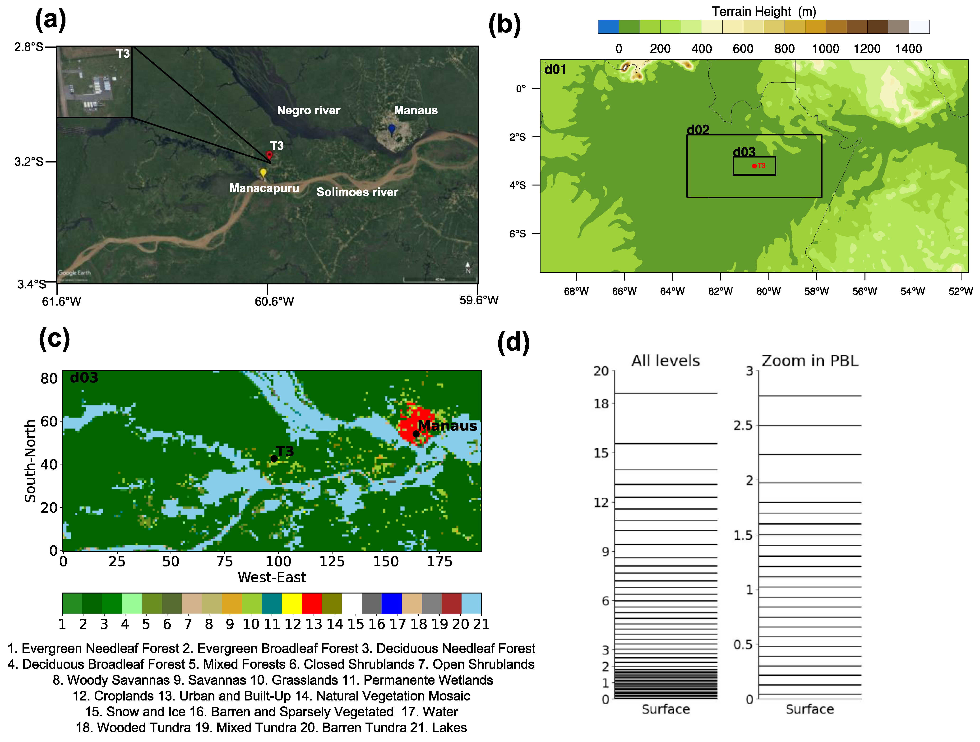
Figure 1. (a) Satellite image of the study area in December 2014 and an aerial view taken over the T3 site in February 2014; (b) the model domain contoured by topography from parent domain (d01); (c) the innermost domain (d03), showing land-use and soil categories in the central Amazon basin; and (d) model vertical levels highlighting the resolution within PBL (Y-axis unit is km).
Atmosphere 14 00850 g001
Figure 2. (a) Comparison of model-predicted (eight PBL schemes) and AOSMET observations [40] for 2-m air temperature (°C), (b) 2-m air relative humidity (%), (c) 10-m wind speed (m·s−1), and (d) precipitation (mm/h) from 30 September to 2 October 2014, starting at 08 LT (X-axis is date and local time). Results from local (nonlocal) PBL schemes are plotted with filled (dashed) lines. The colors of the bars in subfigure (d) follow the legend.
Atmosphere 14 00850 g002
Figure 3. (a) Comparison of model-predicted (eight PBL schemes) and AOSMET observations [40] for 2-m air temperature (°C), (b) 2-m air relative humidity (%), (c) 10-m wind speed (m·s−1), and (d) precipitation (mm/h) from 14 to 16 October 2015, starting at 08 LT (X-axis is date and local time). Results from local (nonlocal) PBL schemes are plotted with filled (dashed) lines. The colors of the bars in subfigure (d) follow the legend.
Atmosphere 14 00850 g003
Figure 4. (a) Comparison of model-predicted (8 PBL schemes) and 30ECOR observations [41] for sensible heat flux (W·m−2), (b) latent heat flux (W·m−2), and (c) friction velocity (m·s−1) from 30 September to 2 October 2014, starting at 08 LT (X-axis is date and local time). Results from local (nonlocal) PBL schemes are plotted with filled (dashed) lines. The black dots in subfigure (c) are the available measurements for friction velocity.
Atmosphere 14 00850 g004
Figure 5. (a) Comparison of model-predicted (8 PBL schemes) and 30ECOR observations [41] for sensible heat flux (W·m−2), (b) latent heat flux (W·m−2), and (c) friction velocity (m·s−1) from 14 to 16 October 2015, starting at 08 LT (X-axis is date and local time). Results from local (nonlocal) PBL schemes are plotted with filled (dashed) lines. The black dots in subfigure (c) are the available measurements for friction velocity.
Atmosphere 14 00850 g005
Figure 6. (a) Comparison of model-predicted (8 PBL schemes) and SONDEWNPN sounding observations [42] for potential temperature (K), (b) vapor mixing ratio (g·kg−1), and (c) horizontal wind speed (m·s−1) at 02 (first row), 08 (second row), 14 (third row), and 20 LT (fourth row) for 1 October 2014. Results of local (nonlocal) PBL schemes are represented by filled (dashed) lines.
Atmosphere 14 00850 g006
Figure 7. (a) Comparison of model-predicted (8 PBL schemes) and SONDEWNPN sounding observations [42] for potential temperature (K), (b) vapor mixing ratio (g·kg−1), and (c) horizontal wind speed (m·s−1) at 02 (first row), 08 (second row), 14 (third row), and 20 LT (fourth row) for 15 October 2015. Results of local (nonlocal) PBL schemes are represented by filled (dashed) lines.
Atmosphere 14 00850 g007
Figure 8. Comparison of model-predicted (8 PBL schemes), CEILPBLHT observations [42] (OBSCEIL), and estimated from radiosonde soundings (OBSRS) for planetary boundary layer height (m) from 30 September to 2 October 2014, starting at 08 LT (X-axis is date and local time). Results from local (nonlocal) PBL schemes are plotted with filled (dashed) lines.
Atmosphere 14 00850 g008
Figure 9. Comparison of model-predicted (8 PBL schemes), CEILPBLHT observations [42] (OBSCEIL), and estimated from radiosonde soundings (OBSRS) for planetary boundary layer height (m) from 14 to 16 October 2015, starting at 08 LT (X-axis is date and local time). Results from local (nonlocal) PBL schemes are plotted with filled (dashed) lines.
Atmosphere 14 00850 g009
Figure 10. (a) Taylor diagram (left) and Taylor skill score chart (right) showing the performance of evaluated PBL schemes for T2, (b) RH2, (c) U10, (d) H, (e) LE, and (f) PBLH prediction for the 2014 period. The azimuthal angle represents the correlation coefficient, and the radial distance is the standard deviation normalized to the observations (black dot above the X-axis). The colors for each PBL scheme are ACM2 (yellow), MRF (orange), SH (lime), YSU (salmon), BouLac (green), GBM (blue), MYNN2.5 (cyan), and UW (teal).
Atmosphere 14 00850 g010
Figure 11. (a) Taylor skill score for predicted PBLH at daytime (left) and nighttime (right) for the 2014 study period (top-row) and (b) for the 2015 study period (bottom-row).
Atmosphere 14 00850 g011
Figure 12. Taylor diagram (left) and Taylor skill score chart (right) showing the performance of evaluated PBL schemes for (a) T2, (b) RH2, (c) U10, (d) H, (e) LE, and (f) PBLH prediction for the 2015 period. The azimuthal angle represents the correlation coefficient, and the radial distance is the standard deviation normalized to the observations (black dot above the X-axis). The colors for each PBL scheme are ACM2 (yellow), MRF (orange), SH (lime), YSU (salmon), BouLac (green), GBM (blue), MYNN2.5 (cyan), and UW (teal).
Atmosphere 14 00850 g012
Table 1. Statistical indexes employed to performance evaluation.
IndexesEquations *
Mean Bias (MB) M B = 1 N k = 1 N f k o k = f o
Root mean square error (RMSE) R M S E = 1 N k = 1 N f k o k 2 1 / 2
Correlation coefficient (r) r = k = 1 N f k f o k o k = 1 N f k f 2 1 / 2 k = 1 N o k o 2 1 / 2
Index of agreement (IOA) I O A = 1 1 N k = 1 N O k f k 2 k = 1 N f k o + o k o 2
Taylor skill score (TSS) T S S = 2 1 + r σ ^ + 1 / σ ^ 2
* N is the number of samples, f is the forecasting data, o is the observational data, and σ ^ = (σfcstobs).
Disclaimer/Publisher’s Note: The statements, opinions and data contained in all publications are solely those of the individual author(s) and contributor(s) and not of MDPI and/or the editor(s). MDPI and/or the editor(s) disclaim responsibility for any injury to people or property resulting from any ideas, methods, instructions or products referred to in the content.