Article

Space-Time Causality Analysis of Regional Impacts of ENSO on Terrestrial and Oceanic Precipitation

by
Gleisis Alvarez-Socorro
1,
José C. Fernández-Alvarez
1,2 and
Luis Gimeno
1,*
1
Environmental Physics Laboratory (EPhysLab), Centro de Investigación Mariña, Universidade de Vigo, 32004 Ourense, Spain
2
Departamento de Meteorología, Instituto Superior de Tecnologías y Ciencias Aplicadas, Universidad de La Habana, La Habana 10400, Cuba
*
Author to whom correspondence should be addressed.
Atmosphere 2023, 14(5), 841; https://doi.org/10.3390/atmos14050841
Submission received: 24 March 2023 / Revised: 3 May 2023 / Accepted: 7 May 2023 / Published: 9 May 2023
(This article belongs to the Section Meteorology)

Abstract

:
Future changes are expected in precipitation under climate change, therefore, changes are projected in the oceanic and terrestrial components. However, it remains poorly elucidated how the El Niño–Southern Oscillation (ENSO) can influence these changes. Therefore, we aimed to perform a space-time causality analysis of regional ENSO impacts on terrestrial and oceanic precipitation by using the Granger causality method as a function of eight temporal lags (lags 1–8). The monthly values of total precipitation obtained using the Lagrangian approach and their respective terrestrial (PLT) and oceanic (PLO) components were used. The analysis was performed for the two regions of western North America (WNA) and eastern South America (ESA) with strong ENSO signals. For the WNA region in winter, the maximum Granger causality was observed in the component of oceanic origin for temporal lags 1 and 2 (3 and 6 months), with a predominance of both positive and negative ENSO conditions. For the ESA region, it was verified that the causality of the ENSO index was maximum for PLT. Temporal lags 2–5 (6–15 months) stood out in winter when there was a marked region of the Granger causality over the La Plata Basin. In autumn, for lags 1–4 (3–12 months), the Granger causality values were predominant in the southern and western areas of ESA and showed a tendency to move northward with an increased temporal lag. Finally, it was shown that high correlation values did not imply the causality of the relationship between the ENSO index and precipitation in the two regions.

1. Introduction

The hydrological cycle is highly complex [1], and detailed analysis in the context of climate change is very important in the scientific community. Basic thermodynamic and energetic considerations (e.g., the Clausius–Clapeyron relationship) suggest that an increase in global mean surface temperature implies an increase in atmospheric moisture content [2,3,4,5]. This process occurs because the atmosphere exhibits an enhanced water-holding capacity. Therefore, an increase in the mean precipitation pattern, extreme values, and evaporation–precipitation balance is expected. In particular, the percentage of precipitation of oceanic origin is projected to rise with greater importance of oceanic moisture sources in the future climate [1].
However, under conditions where notable modifications in the atmospheric circulation pattern are not observed, an increased transport is expected from divergent to convergent regions. Therefore, in subtropical oceans, the most important divergent regions and continents mostly behave as convergent regions, which determines that the contribution of oceanic precipitation will rise [6]. It is known that limitations in the availability of soil moisture influence soil evaporation, implying decreased importance of precipitation of terrestrial origin as opposed to oceanic origin. Numerical simulations have accurately projected that the global recycling rate of moisture decreases by ~2–3% per a 1 °C temperature rise [7]. Therefore, individually analysing changes in the components of precipitation (its oceanic and terrestrial origin) will allow for a more accurate understanding of modifications in the hydrological cycle, thus distinguishing the effects of short-to-long-term impacts. This analysis is crucial for implementing prevention/adaptation measures, reducing vulnerability, and mitigating risk.
In particular, Gimeno et al. [1] used a Lagrangian approach to study the behaviours of oceanic (PLO) and terrestrial (PLT) precipitation components and observed a significant increase in the current climate of PLO, which was greater in tropical areas. Terrestrial precipitation was of increased importance for regions, such as the Amazon and Central Equatorial Africa, given the increased PLO. Sori et al. [8] demonstrated that PLT represents > 50% of the total precipitation determined using the Lagrangian approach (PL) in most PLO and PLT analyses for river basins. These results confirm the importance of precipitation recycling and moisture transport in continental regions. Additionally, Sori et al. [8] highlighted the importance of PLO in almost all North American river basins. However, these studies have focused on PLO and PLT changes but have not analysed how these changes might be influenced by the El Niño–Southern Oscillation (ENSO) and which regions show the most significant changes. Therefore, these studies did not determine the causality of the ENSO for the components of precipitation.
Several studies have used the Granger causality method to analyse climate teleconnections by using different variables, such as surface temperature [9], terrestrial evaporation [10], total precipitation [11], global evaporation [12] and global dust activities [13]. These studies demonstrate the ability of this statistical method to analyse the causality of teleconnection patterns for a given variable. However, the approach proposed by these studies has not been applied to determine the space-time causality of the ENSO for PLO and PLT on regional or global scales.
Therefore, the specific objectives of this study were to (1) analyse the space-time causality of the ENSO impacts on oceanic and terrestrial precipitation at two specific regions as a function of different temporal lags via the Granger method; and (2) compare results with the correlation pattern found for the same temporal lags. The latter is of utmost importance since many studies have associated changes in precipitation with the ENSO index based on the coefficient of correlation. However, the correlation pattern is a statistical measure that describes the strength and direction of a linear relationship between pairs of variables, and therefore, does not determine causality [14].

Study Regions

To carry out the study, two study regions were selected that satisfied the following criteria: (1) there is an ENSO climatic signal that affects the total precipitation pattern; and (2) values of an oceanic or terrestrial precipitation component associated with some mechanism of moisture transport are prevalent, such as atmospheric rivers (ARs) or low-level jets (LLJs).
The first study area corresponded to western North America (WNA); namely, only the region delimited by the red rectangle [100–130° W, 34–52° N] (Figure 1a). This region corresponded to the area of maximum influence of ARs that make landfall in winter [15,16]. The ENSO affects the overall variability of interannual precipitation in this region [17,18,19]. In particular, for El Niño winters, increased precipitation was observed in the extreme southern United States (US), whereas increased dry conditions were observed in the mid-latitudes of the US. According to Payne and Magnusdottir [20], the ENSO influences the landfalling ARs (LARs) in this region. In general, the maximum and minimum numbers of LARs occur for El Niño and La Niña, respectively, causing a latitudinal shift towards the equator in the positive phase and the opposite (towards higher latitudes) in the negative phase. Finally, during El Niño winters, the total precipitation anomalies were positive in the coastal areas of California. During La Niña winters, the contribution of the AR group decreases, showing negative precipitation anomalies [21].
The second study region (Figure 1b) was defined around the La Plata Basin, that is, eastern South America (ESA) [40–70° W, 15–38° S]. Its selection was based on the fact that several studies have shown that the ENSO impacts occur during boreal winter (December–February) and boreal autumn (September–November) [22,23,24]. However, the South American low-level jet (SALLJ) influences ESA and is the main mechanism contributing to moisture transport over South America (e.g., [25,26]), in particular, over the La Plata Basin (LPB). The SALLJ transports a large amount of moisture along the eastern edge of the Andes towards the southern Amazon Basin and La Plata River Basin. In addition, the SALLJ can be modulated by the ENSO, influencing the total precipitation. For example, Ferreira et al. [27] and Marengo et al. [28] showed that the SALLJ was stronger and more frequent during the El Niño summer of 1998 than during the La Niña summer of 1999, contributing twice as much precipitation. Montini et al. [26] indicated that SALLJ days were more frequent during the winter and summer of El Niño years than during neutral years. In addition, SALLJ days were significantly less frequent during the autumn than during the other seasons of La Niña years but showed no significant difference between winter and summer for La Niña. Montini et al. [26] summarised that the frequency of the SALLJ in both regions increases (decreases) during El Niño (La Niña) events.

2. Data and Methods

2.1. Data Used

In this study, the monthly values of Lagrangian precipitation (PL) and its oceanic (PLO) and terrestrial (PLT) components determined by Nieto and Gimeno [29] for 1981–2018 were used. A detailed analysis of the experiments conducted to obtain this database can be found in Nieto and Gimeno [29,30] and Sori et al. [8]. It should be noted that PL and its components of PLO and PLT are approximations of real precipitation. Specifically, PL, PLO, and PLT are calculated using the results of global modelling using the Lagrangian particle dispersion model (FLEXPART v9.0) [31,32] forced with ERA–Interim reanalysis for the period from 1980 to 2018. In particular, PLO and PLT were considered to analyse the influence of the ENSO on precipitation of terrestrial and oceanic origin in the study regions for different temporal lags. The spatial resolution of the data was 0.25° × 0.25°. This database was advantageous for this type of analysis on a regional scale since it was determined considering the optimal monthly integration times for each region, allowing us to consider the water vapour residence times for each specific region.
The monthly values of Multi-Source Weighted–Ensemble Precipitation (MSWEP) v2.8 [33] were also considered real precipitation. The temporal and spatial resolutions of MSWEP were 3 h and 0.1° × 0.1°, respectively. It should be noted that MSWEP is a product obtained from a rain gauge, satellite, and reanalysis, achieving a highly accurate estimate of precipitation at each grid point. Therefore, MSWEP is expected to show better representation than other precipitation products in both densely gauged and ungauged regions. These data were interpolated to a resolution of 0.25° × 0.25° so that they had the same resolution as the Lagrangian precipitation. In particular, MSWEP is mainly used as a reference for the evaluation of precipitation components determined using the Lagrangian approach. Finally, to carry out the causality analysis, the Bivariate ENSO Index (BEST) was used to represent the ENSO conditions. The approach was based on the BEST lead, which combines the sea surface temperature (SST) Niño 3.4 index and the Southern Oscillation Index, as opposed to other indices that rely on only SST data or the atmospheric component [34].

2.2. Granger Causality Method

The Granger causality method was used to analyse the regional impacts of the ENSO on the precipitation components. In this study, it was calculated using a vector autoregressive (VAR) model as follows:
y(t) = c0 + c1 × y(t − 1) +⋯+ ck × y(t − k) + εt,
y(t) = a0 + a1 × y(t − 1) + ⋯+ ak × y(t − k) + bl × x(t − l) + ⋯+ bn × x(t − n) + εt,
The VAR method considers two regressions for model fit. Exactly, it employs a regression function on the prediction and based on its lagged values as shown in Equation (1) [e.g., y (t − 1) … y (t − k)] and another regression that predicts y as a function of lagged values of x [e.g., x (t − l) … x (t − n)] and the lagged value of y (Equation (2)) [11]. Furthermore, the variables c0 or a0 are vectors of constants that serve as the intersection of the model and εt is a vector k of error terms. Finally, ak, ck and bk is a time-invariant matrix. In Equation (2), l is the shortest lag and n is the longest, for which the lag value of x is significant.

VAR Formulation

As a specific case of the autoregressive model, VAR is used to analyse the relationship between several variables. Song et al. [11] provided a detailed explanation of this mathematical formulation. In general, if we have two time series, x, and y, we can apply the Granger causality test of x and y by varying the lag order (p). Lag selection is described in the next section. To test for statistical significance when the Granger causality of x and y is applied, the F-test is used. This test provides two values: test statistic and critical value. For this, we considered the null hypothesis that y is not Granger caused by x and the alternative hypothesis that y is Granger caused by x. The F-test is defined as follows:
f = ( R u 2 R γ 2 ) / γ R u 2 / ( θ δ )
where R2 is the coefficient of determination; R2u is the R2 value of the unrestricted regression model in Equation (2); R2γ is the R2 value of the restricted regression model in Equation (1); γ is the number of restrictions; θ is the number of observations; and δ is the number of explanatory variables in the unrestricted model. In the F-test, the f statistic follows the F-test distribution under the null hypothesis [11]. Based on the results obtained for the F-test, it is true that Granger causality exists when the test statistic > critical value. This consideration is equivalent to a p-value < α; therefore, the null hypothesis is rejected, resulting in that y is Granger caused by x. When the Granger Causality method is used, it should be noted that the test is not true causality, but predictive causality [35]. That is, the time series are temporally related. Thus, if the prediction of future values of a time series y(t) is improved by including past values of a time series x(t), x(t) is said to be “Granger cause” y(t). This study considered a significance level of 95% [11]. The Python Stats Models library [36] was used to develop the research and application of the VAR method.

2.3. Methodology

The results of this study corresponded to the period of 1981–2018. To use the Granger causality method and correlation, the winter (DJF), spring (MAM), summer (JJA), and autumn (SON) time series were constructed for each grid point corresponding to MSWEP, PL, PLT, and PLO. Subsequently, the seasonal ENSO series was built considering the temporal lag to be used. In this case, eight temporal lags were considered, which represented two years backward in time for the year in which it began. We define the temporal lags as shown in Table 1. Therefore, the correlations of MSWEP, PL, PLT, and PLO with the ENSO were determined for each temporal lag in both areas. In addition, statistical significance was analysed to establish the areas of interest from the correlation pattern. That stands out: regions with observed positive (negative) correlations indicate that El Niño is related to an increase (decrease) in precipitation. Conversely, in regions where the correlation is negative (positive), La Niña favours an increase (decrease) in precipitation [37]. Then, the results for Granger causality were analysed and compared with those shown by the correlation pattern. In the results, emphasis was placed on PLO and PLT as they constituted our main objective; however, a comparison of PL and MSWEP was made for the Granger causality and correlation values to demonstrate that the results shown were reliable. This process was because the results obtained for PL, PLT, and PLO were the Lagrangian approximations of precipitation.

3. Results and Discussion

3.1. Correlation and Granger Causality for WNA Region

To compare with the Granger causality model, we also calculated the correlation of the ENSO index with PL, MSWEP, PLO, and PLT for the eight temporal lags (1–8) (Figures S1–S4 in the Supplementary Material). In addition, a comparative analysis was carried out for the number of points with positive and negative correlations in the selected area, and a similar analysis was performed for those that were statistically significant at 95%, which were framed by contours. Figures S1 and S2 show the spatial representation of the correlation pattern (R) for PL and MSWEP. It can be stated that there was a similarity in the regions of the positive and negative correlations; therefore, the results shown below for both precipitation components were reliable compared with the results shown for MSWEP. In particular, Figures S3 and S4 correspond to the correlations for PLT and PLO, respectively. It was observed that, for PLT, there were very low correlations for the ENSO index in the entire region analysed and for all the temporal lags. For PLO, regions with the positive and negative values R predominated for lags 1 and 2, distributed to the south and north of the WNA region, whereas, for lags 3–5 and 8, R was mostly positive with a pattern that extended from the coast to the centre of the area, with a maximum near the Pacific Ocean. McGraw and Barnes [9] found maximum values of R for periods longer than seven months (lag 3) for this region. Son et al. [11] demonstrated a positive correlation in the WNA region for a temporal lag of seven months.
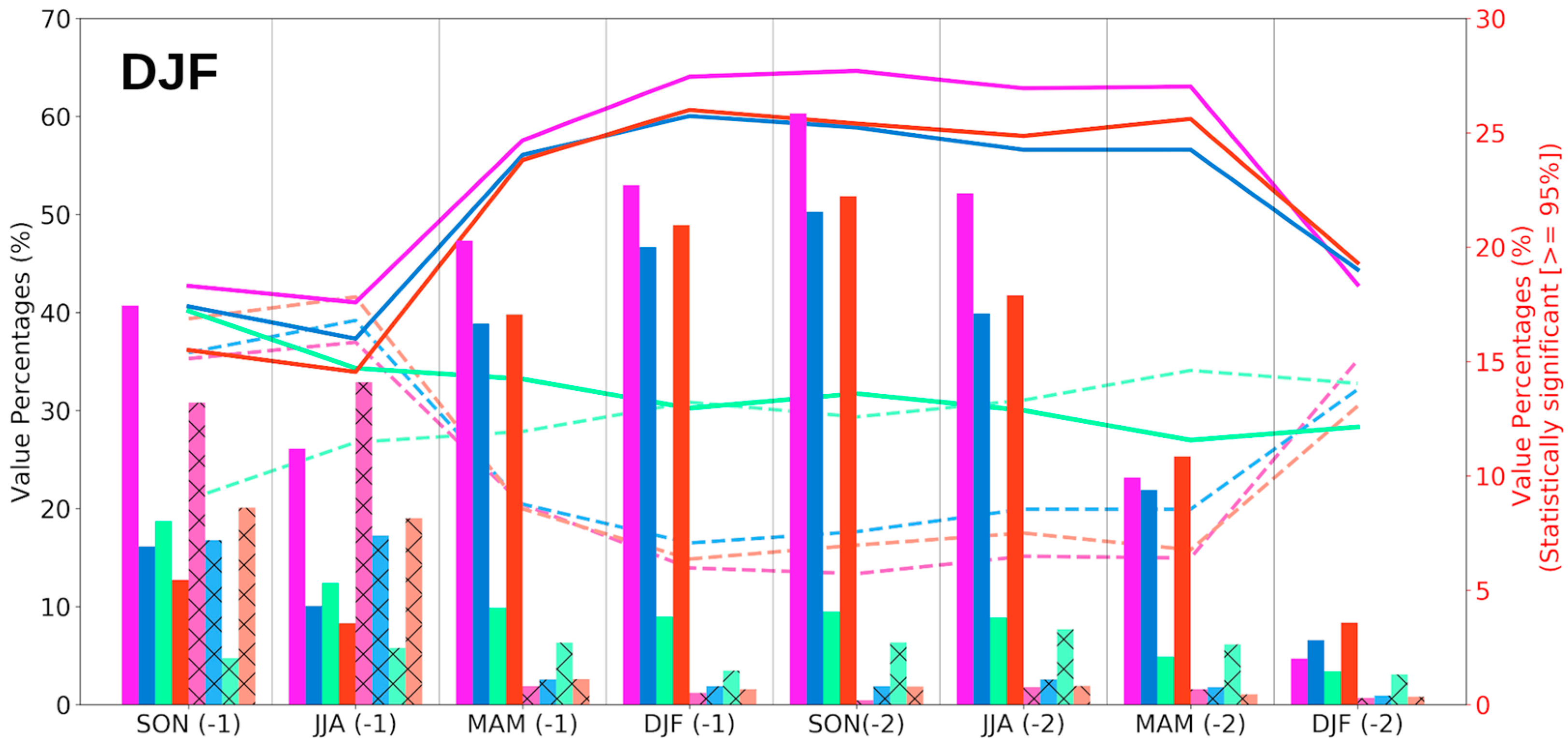
A percentage summary of how the points with the positive and negative R values for WNA change for each temporal lag is shown in Figure 2 (left axis). In this case, the colours are associated with each database used, and the solid and dashed curves are points with positive and negative R, respectively. For temporal lags 1 and 2, a highly similar percentage of points with positive and negative R values existed within a range of 35–45%. However, there was a difference in the percentage of points with positive R (>40%) versus negative R (<30%) for the rest of the temporal lags. It should be noted that the percentage values showed a constant value of ~30% for PLT (solid green line), significantly differing from PLO, MSWEP, and PL, for temporal lags 3–7. The percentage of points with positive or negative R values at p-value < 0.05 is shown in the same graph (right axis). In this case, the marked bars correspond to points with a negative R-value, with the rest being points with a positive R-value. Overall, the largest difference existed for the temporal lags of 9–21 months, predominantly for the positive R. Therefore, increased statistical significance of the ENSO index for winter precipitation existed over WNA for the positive R in the periods of the spring of the previous year until two years ago. Though relatively higher for the negative R, a range of 5–10% of points with both positive and negative R values at p-value < 0.05 existed for lags 1 and 2.
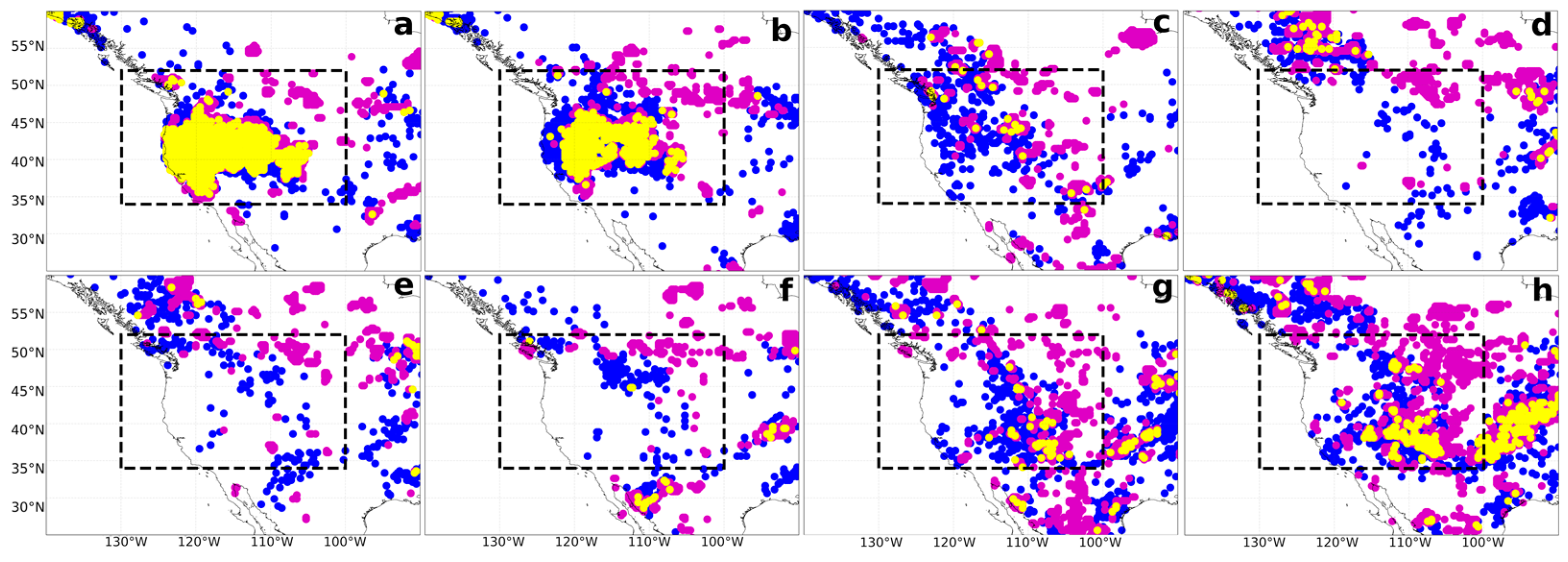
Since this correlation analysis does not show if there is a causality of the ENSO index for the precipitation pattern, we performed an analysis similar to the one shown below. In particular, for the WNA region, the analysis was carried out for the winter season, when the signal was at its maximum. First, the results obtained using the Granger method for the PL and MSWEP data were compared. Figure 3 shows the points within the study region considered and the Granger causality of the ENSO index for PL (blue) and MSWEP (magenta). Figure 3a–h represents temporal lags 1–8, respectively, by which the method was applied (Table 1). Figure 3 shows the yellow dots which corresponded to the regions where the Granger causality of the ENSO index for both PL and MSWEP coincided. An overall similarity existed in the point distribution for both databases, which was better for lags 1 and 2 than for the other lags. For the remaining temporal lags, although the number of points declined, some differences occurred with the increasing temporal lag. Therefore, for this region, the representation of the Granger causality for precipitation with the Lagrangian approach was highly similar to the results obtained using a real precipitation database (in this case, MSWEP).
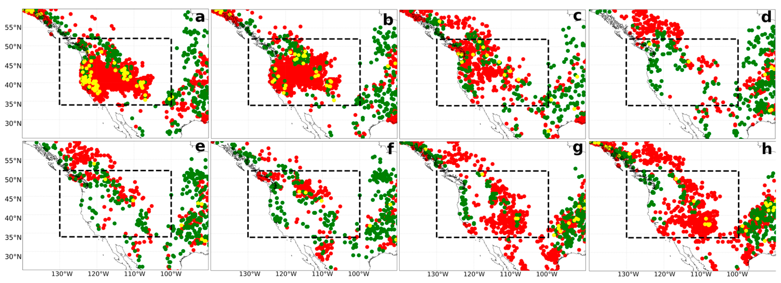
Figure 4 shows the results of the Granger causality of the ENSO index for PLO (red) and PLT (green). The coincident points are indicated in yellow. The increased Granger causality of the relationship between PLO and ENSO prevailed in most of the selected regions, being maximum for lags 1 and 2. This result pointed to a maximum influence of the ENSO on the PLO pattern for 3–6 months in this region. The ENSO causality declined with the lags from 9 to 18 months. For the lags of 21–24 months, a higher number of points showed a significant Granger causality for areas further away from the coast. The effect of the ENSO on PLT in this region was practically negligible. This may be related to the fact that, in this region, in particular, for winter, precipitation is associated with the movement of ARs from the Pacific to the US coast [20]. Finally, few areas existed where the Granger causality of the ENSO index for PLO and PLT coincided in this region. Therefore, although there were maximum R values for the temporal lags of 9–18 months, this did not result in the Granger causality of the ENSO index for precipitation, in particular, for PLO. This region exhibited the maximum Granger causality of 3–6 months. This result was in agreement with the result of Son et al. [11] that no Granger causality of the ENSO index was found for surface precipitation for a temporal lag of seven months in this region.

3.2. Correlation and Granger Causality for ESA Region

Similar to the analysis conducted for R, Granger causality corresponding to the WNA region was performed in this section for ESA. In this case, two seasons (winter and autumn) were analysed based on previous studies, where the influence of the ENSO on precipitation in this region was determined. The R pattern was verified to be similar for MSWEP and PL (Figures S5, S6, S9 and S10) in both seasons. Therefore, the results for this region with PLT and PLO were reliable. For the ESA region, in both seasons, the R values of ENSO vs. PLO were very low and not significant (Figures S8 and S12). However, for PLT, both maximum positive and negative R values were observed. In particular, in winter for this region, the positive R values predominated in most of the temporal lags, except for lag 7–8. Notably, for lags 1–3, a region of the positive R-value around the LPB and a smaller region of the negative R-value near the Cordillera de Los Andes prevailed (Figure S7). Finally, for lags 7–8, the negative R values were observed, showing a relationship between the La Niña phase and PLT.
Though more accentuated around the LPB, the negative R values predominated in most of the area for autumn. However, the band of the positive R values extended further north from the Cordillera de Los Andes range to approximately the coast. This behaviour may be associated with the strengthening of the SALLJ during autumn in the warm phase of El Niño in this region [27,28]. It should be noted that, for lag 1, the positive R values predominated and were significant in most of the regions (p-value < 0.05). The results for the R pattern for lag 3 (7–9 months) were similar to those of Son et al. [11] for a maximum correlation lag of seven months. They found a positive R with a predominance of the ENSO warm phase to the north of the LPB and observed this pattern for both winter and autumn (less noticeable) in that area.
Figure 5 shows the percentage summary for ESA in both seasons, with an analysis similar to that in Figure 2. In this case, the behaviour of both seasons was quite similar, highlighting the percentage values associated with the positive relationship between the ENSO and precipitation, relatively lower for the negative R, for lags 1 and 2. However, for the lags of 3–6 months, La Niña conditions predominated in this region and were highly accentuated for autumn with temporal lags of 7–8 (21–24 months). It was verified that the relationship between the ENSO and PLO did not show a significant change in the entire study period analysed in this region. In terms of statistical significance, in both seasons, the percentage values corresponding to the influence of the ENSO on precipitation for lags 1 and 2 were the most important in this region. However, for lags 6–8, the statistical significance for the negative R predominated (La Niña conditions influenced precipitation).
As for the results of Granger causality, Figure 6 shows a comparison of the Granger causality representations for MSWEP and PL. In this region, there were major differences in the results between the two databases. Using Lagrangian precipitation increased the Granger causality of the ENSO index for precipitation in this region. However, for the region more centred in the LPB, there was a similarity between MSWEP and PL mainly for temporal lags 3–5 in winter. In the autumn season, the regions of similarity were most marked for temporal lags 2–6.
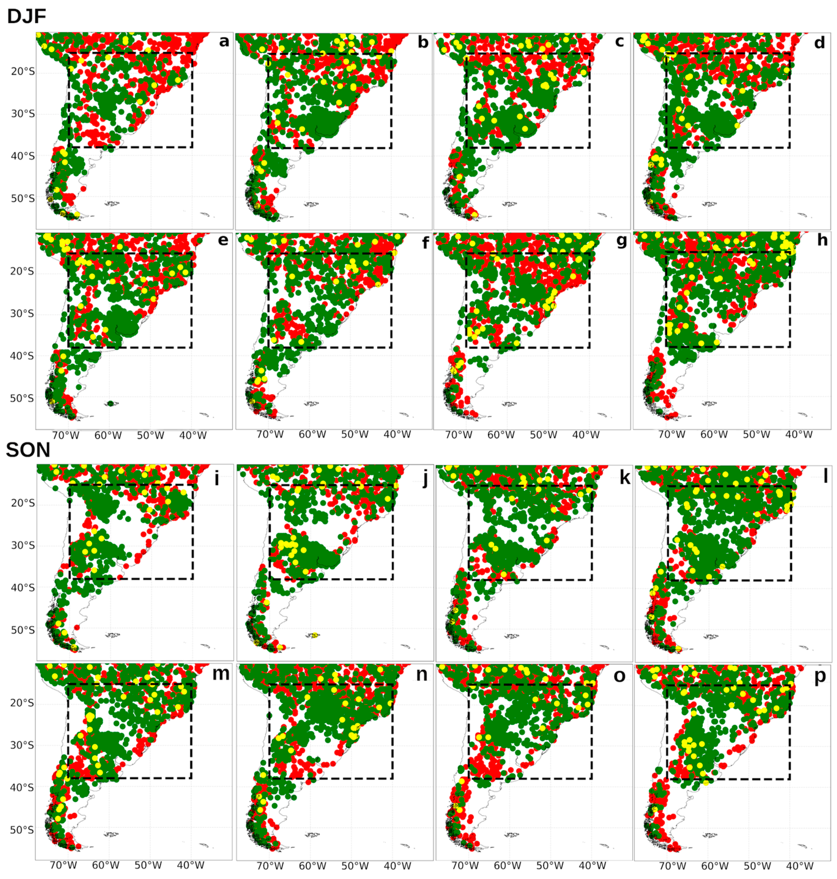
Figure 7 shows the Granger causality of the ENSO index for PLT and PLO in both seasons. For winter, regions with the Granger causality for PLT predominated over PLO, which increased with the longer temporal lags. However, we obtained regions north of the selected area with the ENSO causality for PLO (which may be related to the moisture flux transported by the SALLJ from the Atlantic Ocean [28]. Although there was a maximum positive correlation for lag 1 (3 months) south of the LPB, there was no region where the ENSO causality predominated for PLT or PLO. For temporal lags, 2–5 (6–15 months), the region around the LPB was marked by the influence of the warm phase of the ENSO versus PLT, although it was not significant for the R pattern (p-value > 0.05) (Figure 5). Finally, for lags 6–8, the causality values were distributed to the north and south of the Rio de la Plata, where areas of the positive R predominated, and the causality values where R was negative (i.e., La Niña conditions) decreased significantly.
For autumn, Figure 7 shows that the causality values for PLT in temporal lags 1 and 2 predominated in the southern and eastern regions of the LPB, located at the outer edge of the maximum positive R (Figure S11). In the remaining temporal lags, a shift of these Granger causality values for PLT was observed from south to north, while the correlation was inverse between the ENSO index and PLT for the southern regions, with positive values to the north. However, for temporal lags 3–5, there were areas of Granger causality for the La Niña conditions over the southern and central La Plata basins. The results presented by Son et al. [11] for the Granger causality for seven months (lag 3) showed a significant area in this region. It should be noted that Son et al. [11] used data with a very low spatial resolution compared with those used in this study. The higher spatial resolution leads to a greater spatial distribution in terms of the results and more information on the regions with the Granger causality.

4. Conclusions

In this study, the Granger causality method was used to perform a space-time analysis of the regional impacts of the ENSO on precipitation of terrestrial and oceanic origin. For this purpose, total Lagrangian precipitation and its oceanic and terrestrial components were considered. These were previously determined using the FLEXible PARTicle (FLEXPART) dispersion model forced with ERA–Interim [29]. In this study, the results obtained using Lagrangian precipitation were compared with those obtained using MSWEP. In particular, the influence of the ENSO index on precipitation was studied for the two regions of western North America and eastern South America. In addition, a comparison with the correlation pattern was made to determine if the areas of statistical significance could be detected by the Granger method.
For the WNA region in the winter season, the maximum Granger causality of the ENSO index was found for the component of oceanic origin for temporal lags 1 and 2 (3 and 6 months), with a predominance of the positive and negative ENSO conditions over WNA. However, the Granger causality decreased with the increased temporal lags, where a maximum positive and statistically significant correlation was observed. This result showed that the high correlation did not imply the Granger causality of the ENSO index for precipitation in this region. In addition, the influence of the ENSO on PLT was considered negligible.
For the ESA region, it was verified that the Granger causality of the ENSO index was maximum for PLT. Temporal lags of 2–5 (6–15 months) stood out for winter, where there was a marked region of the Granger causality over the La Plata Basin. This behaviour was associated with a marked influence of the warm phase of the ENSO vs. PLT although the correlation was not significant (p-value > 0.05). A similar behaviour was observed for the rest of the temporal lags. In the autumn season, for lags 1–4, the Granger causality values were predominant in the southern and western areas of ESA, which showed a tendency to move north with lags 5–8, an increase in the most prominent temporal lag. Notably, for temporal lags 3–5, the Granger causality areas existed for the La Niña conditions over the southern and central La Plata basins. In the future, we will study how the position of the SALLJ and ARs influences the distribution dynamics of the correlation and Granger causality values in each region.

Supplementary Materials

The following supporting information can be downloaded at https://www.mdpi.com/article/10.3390/atmos14050841/s1, Figures S1–S4: Correlation patterns of the MSWEP, PL, PLT, and PLO data with the ENSO index for the WNA region in winter; Figures S5–S8: Correlation patterns of the MSWEP, PL, PLT, and PLO data with the ENSO index for the ESA region in winter; Figures S9–S12: Correlation patterns of the MSWEP, PL, PLT, and PLO data with the ENSO index for the ESA region in autumn.

Author Contributions

G.A.-S., J.C.F.-A. and L.G. conceived the idea of the study. G.A.-S. and J.C.F.-A. processed the data and created the figures. G.A.-S. and J.C.F.-A. analyzed the results and wrote the manuscript. All authors analyzed the results and revised the manuscript. All authors have read and agreed to the published version of the manuscript.

Funding

EPhysLab receives partial support from the Xunta de Galicia under the Project ED431C 2021/44 (Programa de Consolidación e Estructuración de Unidades de Investigación Competitivas (Grupos de Referencia Competitiva) and Consellería de Cultura, Educación e Universidade).

Institutional Review Board Statement

Not applicable.

Informed Consent Statement

Not applicable.

Data Availability Statement

Simulations can be obtained by correspondence with the authors.

Acknowledgments

G.A.-S. acknowledge the support from Ministerio de Educación y Formación Profesional under the grants Beca-Colaboración 2022/2023 () and JAE Intro 2022 (JAEINT_22_02769). J.C.F.-A. acknowledge the support from the Xunta de Galicia under the grant no. ED481A-2020/193. This work is supported by the SETESTRELO project (PID2021-122314OB-I00) funded by the Ministerio de Ciencia, Innovación y Universidades, Spain. Partial support was also obtained from the Xunta de Galicia under the project “Programa de Consolidación e Estructuración de Unidades de Investigación Competitivas (Grupos de Referencia Competitiva)” (ED431C 2021/44). G.A.-S., J.C.F.-A. and L.G. thank Rogert Sori and Raquel Nieto for their help in the development of the research. In addition, this work has been possible thanks to the computing resources and technical support provided by CESGA (Centro de Supercomputación de Galicia) and Red Española de Supercomputación (RES) (AECT-2022-3-0009 and DATA-2021-1-0005).

Conflicts of Interest

The authors declare no conflict of interest.

References

  1. Gimeno, L.; Nieto, R.; Sorí, R. The growing importance of oceanic moisture sources for continental precipitation. NPJ Clim. Atmos. Sci. 2020, 3, 27. [Google Scholar] [CrossRef]
  2. Manabe, S.; Wetherald, R.T. On the distribution of climate change resulting from an increase in CO2 content of the atmosphere. J. Atmos. Sci. 1980, 37, 99–118. [Google Scholar] [CrossRef]
  3. Allen, M.; Ingram, W. Constraints on future changes in climate and the hydrologic cycle. Nature 2002, 419, 228–232. [Google Scholar] [CrossRef]
  4. Held, I.M.; Soden, B.J. Robust responses of the hydrological cycle to global warming. J. Clim. 2006, 19, 5686–5699. [Google Scholar] [CrossRef]
  5. O’Gorman, P.A. Contrasting responses of mean and extreme snowfall to climate change. Nature 2014, 512, 416–418. [Google Scholar] [CrossRef]
  6. Huang, J.; Yu, H.; Guan, X.; Wang, G.; Guo, R. Accelerated dryland expansion under climate change. Nat. Clim. Chang. 2016, 6, 166–171. [Google Scholar] [CrossRef]
  7. Findell, K.L.; Keys, P.W.; Van Der Ent, R.J.; Lintner, B.R.; Berg, A.; Krasting, J.P. Rising temperatures increase importance of oceanic evaporation as a source for continental precipitation. J. Clim. 2016, 32, 7713–7726. [Google Scholar] [CrossRef]
  8. Sorí, R.; Gimeno-Sotelo, L.; Nieto, R.; Liberato, M.L.R.; Stojanovic, M.; Pérez-Alarcón, A.; Fernández-Alvarez, J.C.; Gimeno, L. Oceanic and terrestrial origin of precipitation over 50 major world river basins: Implications for the occurrence of drought. Sci. Total Environ. 2023, 859, 160288. [Google Scholar] [CrossRef]
  9. McGraw, M.C.; Barnes, E.A. Memory matters: A case for Granger causality in climate variability studies. J. Clim. 2018, 31, 3289–3300. [Google Scholar] [CrossRef]
  10. Martens, B.; Waegeman, W.; Dorigo, W.A.; Verhoest, N.E.; Miralles, D.G. Terrestrial evaporation response to modes of climate variability. NPJ Clim. Atmos. Sci. 2018, 1, 43. [Google Scholar] [CrossRef]
  11. Song, H.; Tian, J.; Huang, J.; Guo, P.; Zhang, Z.; Wang, J. Hybrid causality analysis of enso’s global impacts on climate variables based on data-driven analytics and climate model simulation. Front. Earth Sci. 2019, 7, 233. [Google Scholar] [CrossRef]
  12. Le, T.; Bae, D.H. Response of global evaporation to major climate modes in historical and future Coupled Model Intercomparison Project Phase 5 simulations. Earth Syst. Sci. Data 2020, 24, 1131–1143. [Google Scholar] [CrossRef]
  13. Le, T.; Bae, D.H. Causal influences of El Niño–Southern Oscillation on global dust activities. Atmos. Chem. Phys. 2022, 22, 5253–5263. [Google Scholar] [CrossRef]
  14. Correlation and Causation. Available online: https://www.abs.gov.au/statistics/understanding-statistics/statistical-terms-and-concepts/correlation-and-causation (accessed on 20 February 2023).
  15. Gimeno, L.; Vázquez, M.; Eiras-Barca, J.; Sorí, R.; Stojanovic, M.; Algarra, I.; Nieto, R.; Ramos, A.M.; Durán-Quesada, A.M.; Dominguez, F. Recent progress on the sources of continental precipitation as revealed by moisture transport analysis. Earth Sci. Rev. 2020, 201, 103070. [Google Scholar] [CrossRef]
  16. Algarra, I.; Nieto, R.; Ramos, A.M.; Eiras-Barca, J.; Trigo, R.M.; Gimeno, L. Significant increase of global anomalous moisture uptake feeding landfalling Atmospheric Rivers. Nat. Commun. 2020, 11, 5082. [Google Scholar] [CrossRef] [PubMed]
  17. Ropelewski, C.F.; Halpert, M.S. North American precipitation and temperature patterns associated with the El Niño/Southern Oscillation (ENSO). Mon. Weather Rev. 1986, 114, 2352–2362. [Google Scholar] [CrossRef]
  18. Yu, J.-Y.; Zou, Y. The enhanced drying effect of Central-Pacific El Niño on US winter. Environ. Res. Lett. 2013, 8, 014019. [Google Scholar] [CrossRef]
  19. Deser, C.; Simpson, I.R.; Phillips, A.S.; Mckinnon, K.A. How well do we know ENSO’s climate impacts over North America, and how do we evaluate models accordingly? J. Clim. 2018, 31, 4991–5014. [Google Scholar] [CrossRef]
  20. Payne, A.E.; Magnusdottir, G. Dynamics of landfalling atmospheric rivers over the North Pacific in 30 years of MERRA reanalysis. J. Clim. 2014, 27, 7133–7150. [Google Scholar] [CrossRef]
  21. Xiong, Y.; Ren, X. Influences of atmospheric rivers on North Pacific winter precipitation: Climatology and dependence on ENSO condition. J. Clim. 2021, 34, 277–292. [Google Scholar] [CrossRef]
  22. International Research Institute for Climate and Society. El Nino and Rainfall Map. Available online: https://iridl.ldeo.columbia.edu/maproom/IFRC/FIC/ElNinoandRainfall.png (accessed on 22 December 2022).
  23. Glantz, M.H.; Naranjo, L.; Baudoin, M.A.; Ramírez, I.J. What does it mean to be El Niño Ready? Atmosphere 2018, 9, 94. [Google Scholar] [CrossRef]
  24. Thomalla, F.; Boyland, M. Enhancing Resilience to Extreme Climate Events: Lessons from the 2015–2016 El Niño Event in Asia and the Pacific. 2017. Available online: https://policycommons.net/artifacts/1359439/enhancing-resilience-to-extreme-climate-events/1972676/ (accessed on 22 December 2022).
  25. do Nascimento, M.G.; Herdies, D.L.; Oliveira de Souza, D. The South American water balance: The influence of low-level jets. J. Clim. 2016, 29, 1429–1449. [Google Scholar] [CrossRef]
  26. Montini, T.L.; Jones, C.; Carvalho, L.M.V. The South American low-level jet: A new climatology, variability, and changes. J. Geophys. Res. Atmos. 2019, 124, 1200–1218. [Google Scholar] [CrossRef]
  27. Ferreira, R.N.; Rickenbach, T.M.; Herdies, D.L.; Carvalho, L.M. Variability of South American convective cloud systems andtropospheric circulation during January–March 1998 and 1999. Mon. Weather Rev. 2003, 131, 961–973. [Google Scholar] [CrossRef]
  28. Marengo, J.A.; Soares, W.R.; Saulo, C.; Nicolini, M. Climatology of the low-level jet east of the Andes as derived from the NCEP-NCAR reanalyses: Characteristics and temporal variability. J. Clim. 2004, 17, 2261–2280. [Google Scholar] [CrossRef]
  29. Nieto, R.; Gimeno, L. Addendum: A database of optimal integration times for Lagrangian studies of atmospheric moisture sources and sinks. Sci. Data 2021, 8, 130. [Google Scholar] [CrossRef]
  30. Nieto, R.; Gimeno, L. A database of optimal integration times for Lagrangian studies of atmospheric moisture sources and sinks. Sci. Data. 2019, 6, 59. [Google Scholar] [CrossRef]
  31. Stohl, A.; James, P. A Lagrangian analysis of the atmospheric branch of the global water cycle. Part I: Method description, validation, and demonstration for the August 2002 flooding in central Europe. J. Hydrometeorol. 2004, 5, 656–678. [Google Scholar] [CrossRef]
  32. Stohl, A.; Forster, C.; Frank, A.; Seibert, P.; Wotawa, G. The Lagrangian particle dispersion model FLEXPART version 6.2. Atmos. Chem. Phys. 2005, 5, 2461–2474. [Google Scholar] [CrossRef]
  33. Beck, H.E.; Wood, E.F.; Pan, M.; Fisher, C.K.; Miralles, D.M.; van Dijk, A.I.; McVicar, T.R.; Adler, R.F. MSWEP V2 global 3-hourly 0.1 precipitation: Methodology and quantitative assessment. Bull. Am. Meteorol. Soc. 2019, 100, 473–500. [Google Scholar]
  34. Smith, C.A.; Sardeshmukh, P. The Effect of ENSO on the Intraseasonal Variance of Surface Temperature in Winter. Int. J. Clim. 2000, 20, 1543–1557. [Google Scholar] [CrossRef]
  35. Granger, C.W.J. Essays in Econometrics: The Collected Papers of Clive W.J. Granger. Cambridge University Press: Cambridge, UK, 2001. [Google Scholar]
  36. Stats Models Statistics in Python. Available online: https://www.statsmodels.org/v0.10.2/ (accessed on 22 December 2022).
  37. Sorí, R.; Nieto, R.; Liberato, M.L.; Gimeno, L. Oceanic versus terrestrial origin of El Niño Southern Oscillation–associated continental precipitation anomalies. Ann. N. Y. Acad. Sci. 2021, 1504, 202–214. [Google Scholar] [CrossRef] [PubMed]
Figure 1. Geographic location of the study regions (region within the red frame): (a) western North America (WNA) and (b) eastern South America (ESA).
Atmosphere 14 00841 g001
Figure 2. Percentage (left axis) of points with the positive (solid lines) and negative (dashed lines) R values in WNA for MSWEP (magenta colour), PL (blue colour), PLT (green colour), and PLO (red colour) as a function of temporal lag [−1 and −2 correspond to one and two years backward in time]. The percentage of those points statistically significant at 95% is shown on the right axis. The marked bars correspond to the negative R-value, with the rest being the positive R-value. Period: 1981–2018.
Atmosphere 14 00841 g002
Figure 3. The subfigures show the points where PL (blue colour) and MSWEP (magenta colour) are Granger, caused by the ENSO index in western North America (WNA). The yellow dots represent regions where the Granger causality of the ENSO index for PL and MSWEP is coincident. (ah) represent temporal lags 1–8, respectively; and period: 1981–2018. The interest region is within the black frame.
Atmosphere 14 00841 g003
Figure 4. The subfigures show the points where PLO (red colour) and PLT (green colour) are Granger caused by the ENSO index in western North America (WNA). The yellow dots represent regions where the Granger causality of the ENSO index for PLO and PLT is coincident. (ah) represent temporal lags 1–8, respectively; and period: 1981–2018. The interest region is within the black frame.
Atmosphere 14 00841 g004
Figure 5. Percentage (left axis) of points with the positive (solid lines) and negative (dashed lines) R values in the ESA area for MSWEP (magenta colour), PL (blue colour), PLT (green colour), and PLO (red colour) as a function of temporal lag [−1 and −2 correspond to one and two years backward in time]. The percentage of those points statistically significant at 95% is shown on the right axis. The marked bars correspond to the negative R-value, with the rest being the positive R-value. (a) winter and (b) autumn. Period: 1981–2018.
Atmosphere 14 00841 g005
Figure 6. The subfigures show the points where PL (blue colour) and MSWEP (magenta colour) are Granger caused by the ENSO index in eastern South America (ESA). The yellow dots represent regions where the Granger causality for PL and MSWEP is coincident. Winter (ah) and autumn (ip). (ah or ip) represent temporal lags 1–8, respectively; and period: 1981–2018. The interest region is within the black frame.
Atmosphere 14 00841 g006
Figure 7. The subfigures show the points where PLO (red colour) and PLT (green colour) are Granger caused by the ENSO index in western North America (WNA). The yellow dots represent regions where the Granger causality of the ENSO index for PLO and PLT is coincident. Winter (ah) and autumn (ip). (ah or ip) represent temporal lags 1–8, respectively; and period: 1981–2018. The interest region is within the black frame.
Atmosphere 14 00841 g007
Table 1. Temporal lag for the ENSO variable for the seasons considered in this study.
Seasons (1983–2018)Lag 1Lag 2Lag 3Lag 4Lag 5Lag 6 Lag 7 Lag 8
DJFSON (1982–2017)JJA (1982–2017)MAM (1982–2017)DJF (1982–2017)SON (1981–2016)JJA (1981–2016)MAM (1981–2016)DJF (1981–2016)
SONJJA (1983–2018)MAM (1983–2018)DJF (1983–2018)SON (1982–2017)JJA (1982–2017)MAM (1982–2017)DJF (1982–2017)SON (1981–2016)
Disclaimer/Publisher’s Note: The statements, opinions and data contained in all publications are solely those of the individual author(s) and contributor(s) and not of MDPI and/or the editor(s). MDPI and/or the editor(s) disclaim responsibility for any injury to people or property resulting from any ideas, methods, instructions or products referred to in the content.