Development of a Computational Fluid Dynamics Model for Ice Formation: Validation and Parameter Analysis

Abstract

In the history of civil aircraft transportation, ice formation has been identified as a key factor in the safety of flight. Anti-icing and deicing systems have emerged through the years with the aim to prevent or to eliminate ice formation on wing airfoils, control surfaces and probes. Modern flying machines demand more efficiency in order to reduce the carbon footprint and increase the sustainability of flight transport. In order to achieve this goal, the need to have an efficient aircraft with an efficient and low power consuming system is fundamental. This paper proposes a new model for ice accretion using computational fluid dynamics (CFD). This model permits the simulation of the shape of the ice formed over a profile varying boundary condition (i.e., speed, liquid water content, and so on). The proposed model also takes into account the amount of heat transferred between the water and the surrounding environment and includes the effects of air turbulence on the ice formation process. The CFD simulations have been validated with NASA experimental outcome and show good agreement. The proposed model can be also used to investigate the effects of various parameters such as air speed, liquid water content, and air temperature on the ice formation process. The results evidence that the proposed model can accurately predict ice formation process and is suitable to optimize the design of anti-icing or deicing systems for aircraft and helicopters. This approach is not limited to aerospace but can also be exported to other applications such as transportation, wind turbine, energy management, and infrastructure.

1. Introduction

Ice accretion poses a significant threat to civil aviation, with severe implications for the safety and performance of aircraft. Numerous studies and investigations [1,2,3,4]. have underscored the dangers that ice formation on external surfaces can present, including a reduced aerodynamic performance, heightened risk of flow separation and stall, compromised authority on control surfaces, and blocked probe inlets. Addressing this challenge is of paramount importance to ensure the safety and efficiency of air travel.

Aircraft icing typically occurs when an airplane or helicopter encounters visible moisture, such as rain or clouds, during flight [5,6]. The specific characteristics of ice formation, including the type of ice that develops, are influenced by factors such as droplet size and air temperature. Understanding the complex interplay of these variables is essential to developing effective strategies for mitigating the risks associated with ice accretion on aircraft surfaces.

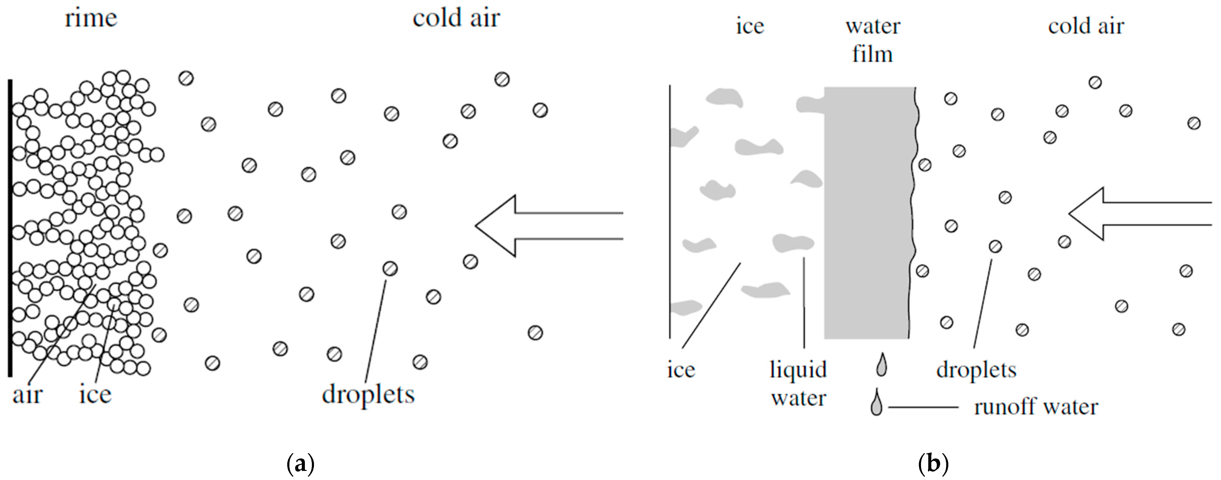
In this context, this study aims to contribute to the ongoing efforts in the scientific community to address the challenges of aircraft icing. By introducing a novel, validated icing model designed to be suitable for anti-icing evaluations, our research seeks to expand the existing body of knowledge on this critical subject and pave the way for future advancements in the field. The three main types are rime, clear, and mixed, here described:

• Rime ice: It forms with air temperatures ranging from −40 °C to −15 °C. Water droplets suspended in air immediately freeze after impact; due to the rapidity, air is trapped inside ice resulting in a white ice, crystalline and brittle. It is easy to remove with deicing system such as inflatable boots. Rime ice seriously can affect the aerodynamic performance due to the irregular horn-shaped protrusions that affect the adhesion of the boundary layer of the airstream [7,8,9].
• Clear ice: It occurs at higher temperatures, ranging from −10 °C to 0 °C with larger, supercooled water droplets. Water remaining liquid runs back as a thin film and progressively freezes. Ice formed has no air cavities and so the final ice appears translucent. Clear ice is considered the most tenacious to remove and the most critical for balancing due to the high density [10,11].
• Mixed ice: between −15 °C and −10 °C, mixed ice forms. It is basically a blend of the previous two with the worst characteristics of both; glaze ice is surrounded by thin feather-shaped rime ice formations [12].

Ice accumulation on an aircraft can led to several adverse effects, including [5,13,14]:

• Increased weight: Ice accumulation on an aircraft’s wings, tail, and other surfaces can increase its weight, which can affect its performance and fuel consumption.
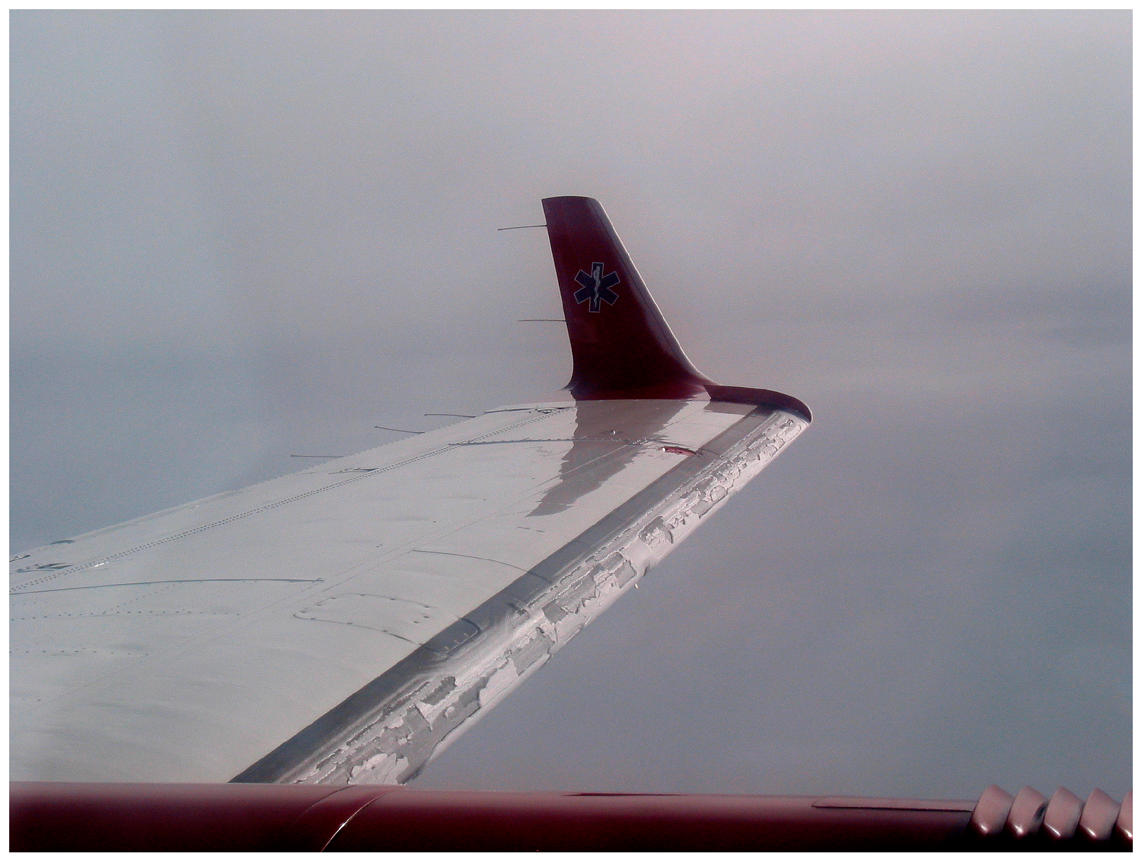
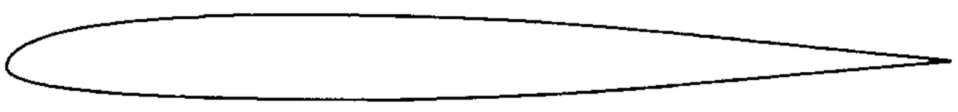
• Reduced lift: Ice can change the shape of an aircraft’s wings (as reported by Figure 1) and reduce its ability to generate lift, which reduces the performance and makes it harder to take off, climb, and maintain altitude.
• Increased drag: Ice can increase the drag on an aircraft’s wings and other surfaces, which can reduce its speed and fuel efficiency.
• Risk of stall: The protrusions created by the ice formation can led to the detachment of the boundary layer and so can induce a stall phenomenon. Furthermore, stall warning systems are designed to operate with clean airfoil. The profile change due to ice accumulation anticipates the stall effect without giving the pilot prodromal advice.
• Loss of control: Ice can affect an aircraft’s control surfaces, such as the ailerons, elevators, and rudder, making it more difficult to maneuver and potentially leading to a loss of control.
• Engine problems: Ice can accumulate on an aircraft’s engines, disrupting their airflow and potentially causing them to malfunction or stall.
• Reduced visibility/air data corruption: Ice accumulation on an aircraft’s windshield, windows, and air data sensors can reduce visibility and corrupt air data (pressure altitude, air speed, and vertical speed), reducing the safety of the flight.

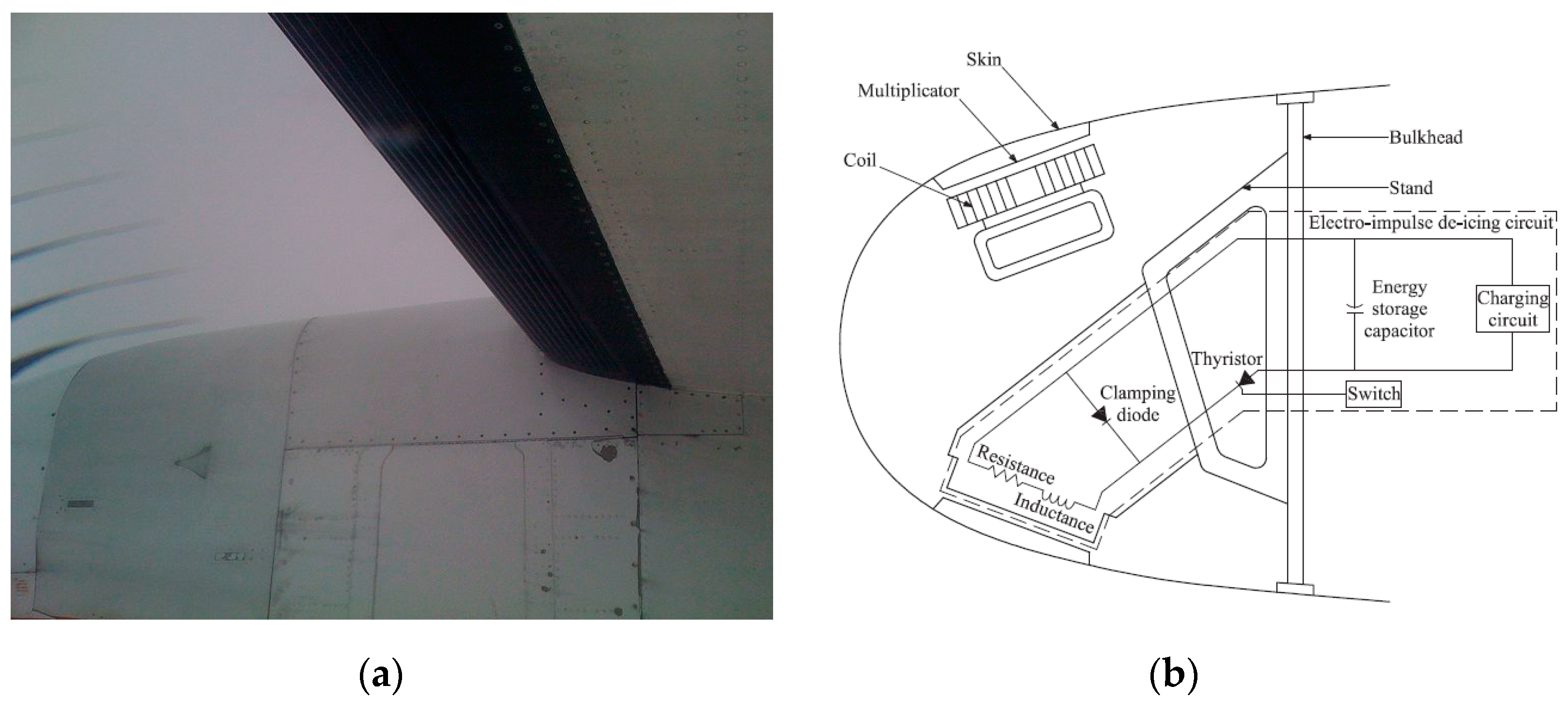
To address this challenge, anti-ice and deicing systems have been developed and refined over time [16]. Deicing equipment is specifically designed to remove ice accumulation using various methods; among the most prevalent are pneumatic boot inflation (schematically illustrated in Figure 2a), thermal heating, and induced vibration of the leading edge (as depicted in Figure 2b). Deicing systems typically operate with an automatically controlled duty cycle, making them particularly well-suited for aircraft with limited excess power available, such as general aviation or commuter aircraft.

One example of a widely installed deicing system is surface deformation deicing. This approach employs technologies such as pneumatic boots [17], which are affixed to the leading edge of the aircraft, or the Electro-Magnetic Impulse Deicing (EIDI) system [18]. These innovations have significantly contributed to enhancing flight safety in icing conditions by effectively mitigating the risks associated with ice accumulation on aircraft surfaces.

Anti-icing systems represent a distinct approach to mitigating the risks associated with ice formation on aircraft surfaces. In contrast to deicing systems, which focus on periodically removing ice accumulation, anti-icing systems are designed to prevent ice formation altogether. Two primary strategies are employed within the anti-icing domain: the low-power-consuming “running wet” approach, which preheats the contact surface sufficiently to inhibit icing, and the “full evaporative” approach, which instantly vaporizes water droplets upon contact with the surface.

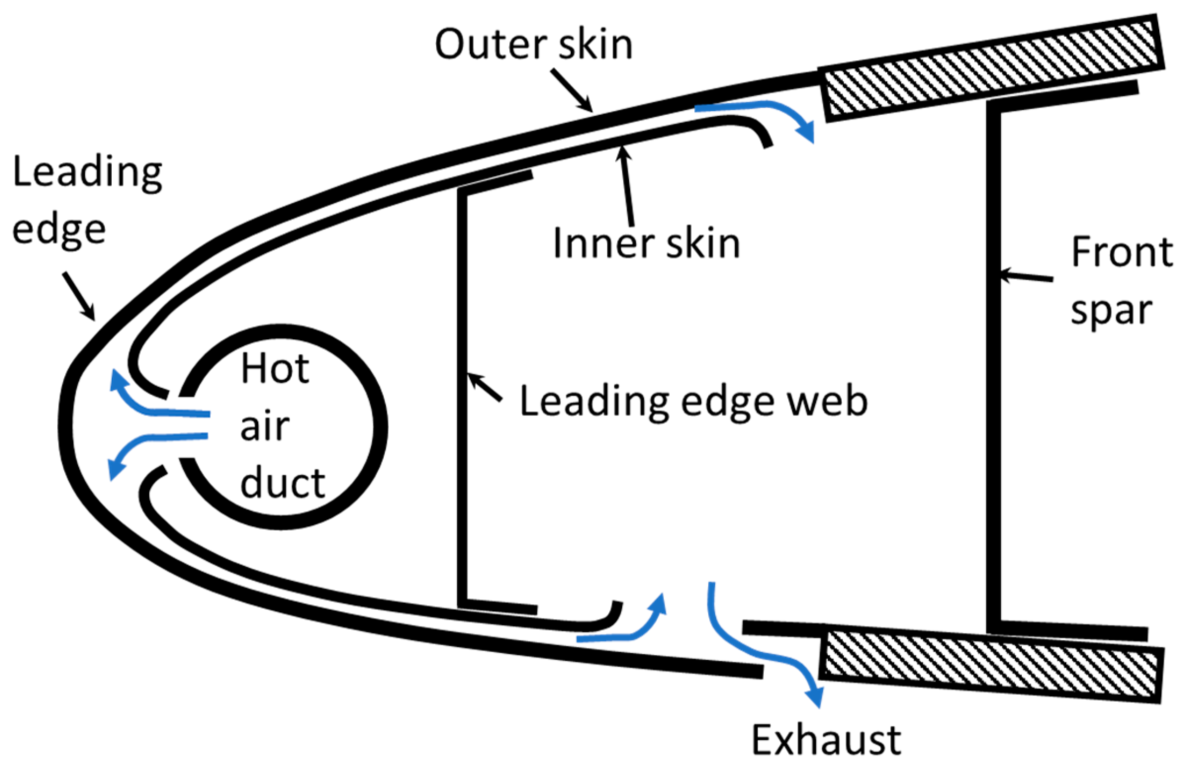
Various power sources are utilized to preheat the leading edge of the wing, with electro-thermal methods being particularly popular in more electric aircraft. These systems rely on a conductive mesh embedded within the composite leading edge panel [21]. Copper meshes have found widespread applications in helicopter blades [22] and on smaller surfaces, such as outside air temperature (OAT) probes or control surfaces. For larger surfaces requiring anti-icing, the prevalent system in use is thermal pneumatic anti-ice. This system leverages turbine compressors or heat exchangers connected to the engine exhaust to supply hot air, which is then distributed via pipes to the aircraft’s leading edges [23]. A schematic section of this system is depicted in Figure 3. A variety of methods may be employed simultaneously on commercial aircraft to address diverse icing positions and devices.

Table 1. Ice location and typical control mode [16].

Ice Location	Control Method
Leading edge of wing	Thermal pneumatic, thermal electric, chemical, and pneumatic (deice)
Leading edges of vertical and horizontal stabilizers	Thermal pneumatic, thermal electric, and pneumatic (deice)
Windshield, windows	Thermal pneumatic, thermal electric, and chemical
Heater and engine air inlets	Thermal pneumatic and thermal electric
Pitot and static air data sensors	Thermal electric
Propeller blade leading edge and spinner	Thermal electric and chemical
Carburetors	Thermal pneumatic and chemical
Lavatory drains and portable water lines	Thermal electric

provides a concise overview of the most common techniques applied in civil liners for different icing locations.

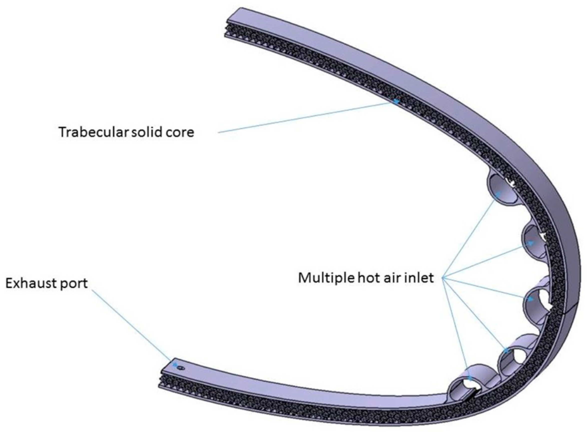
The innovative solution proposed by the authors [24] entails the use of a sandwich panel featuring a lattice core, fabricated using laser powder bed fusion technology. An artistic representation of this concept is presented in Figure 4 which schematically illustrates the novel approach. The design incorporates a sandwich panel with a lattice truss core, serving as both a structural leading edge and an anti-icing system. The component seamlessly integrates internal pipes for hot air passage directly into the skin.

By employing additive manufacturing techniques, it is possible to create this panel in a single piece, eliminating the need for welding or gluing between the core and skins. This innovative approach offers a superior structure, yielding an enhanced performance and durability compared to traditional methods.

This novel solution offers several advantages:

• Thermal efficiency: The air passage inside of the lattice core creates a high turbulence that enhances the heat exchange. Moreover, the punctual control over the lattice permits the customization of the heat diffused where it is needed.
• System efficiency: Integrating the system function inside of the structure permits an important weight saving.
• Reduction in construction and maintenance cost: The panel is recyclable and is a single piece plug and play without the need of welding, joining, or special gluing.
• Easy to rescale and manufacture: This permits the installation of this system even in small scale unmanned aircraft or UAV with an enhancement in the flight safety and operability.

The innovative system introduced in this study allows for the localized customization of heat flux to prevent ice formation or to melt existing ice accumulations. Consequently, it is essential to develop a computational tool capable of accurately simulating ice deposition and accretion while also integrating the necessary local heat input to achieve either a running wet or full evaporative solution. The development of such a tool is critical in optimizing the novel system’s performance and ensuring its effectiveness in mitigating the hazards posed by aircraft icing in a range of conditions.

The field of ice accretion modeling has seen significant progress in recent years, with several key models emerging as the most widely recognized and utilized. Among these, the LEWICE model, developed by NASA Glenn Research Center [25], stands out for its comprehensive treatment of icing physics and its ability to simulate ice accretion on both 2D and 3D surfaces. Another prominent model is the FENSAP-ICE software, which combines the capabilities of the FENSAP panel method for aerodynamic analysis with an advanced icing module [26]. This model is particularly known for its ability to capture complex interactions between the airflow, droplet impingement, and heat transfer processes during ice accretion. Additionally, the CANICE model, developed by the National Research Council of Canada [27], has gained recognition for its extensive validation against experimental data and its use in the certification of aircraft ice protection systems. Collectively, these state-of-the-art ice accretion models have provided valuable insights into the intricate phenomena underlying aircraft icing, laying the groundwork for the development of advanced anti-icing and deicing systems aimed at enhancing aviation safety and efficiency.

The ANSYS FENSAP-ICE software also plays a significant role in advancing our understanding of the complex processes involved in aircraft icing. ANSYS FENSAP-ICE is an evolution of the FENSAP-ICE software [28], which combines the capabilities of the FENSAP panel method for aerodynamic analysis with an advanced icing module. ANSYS FENSAP-ICE enhances the original model by incorporating cutting-edge computational fluid dynamics (CFD) and heat transfer analysis tools provided by the ANSYS suite. This allows for more accurate and detailed simulations of the airflow, droplet impingement, and heat transfer processes that occur during ice accretion on aircraft surfaces.

The development of a new ice accretion model that integrates both anti-icing and deicing systems that will be specifically tailored for lattice core sandwich panels represents a significant step forward and a scientific improvement in the field of aircraft icing, offering potential improvements in aircraft safety, efficiency, and structural performance.

2. Materials and Methods

Currently there are several codes developed by different countries:

• LEWICE (USA) [27];
• FENSAP-ICE (Canada) [26];
• CAPTA (France) [29];
• MULTIICE (Italy) [30]; and
• TRAJICE (UK) [31].

In this paper, a novel ice formation model will be implemented using STAR-CCM + software. The novelty of this tool is in the capability to extrapolate the amount of heat needed to prevent ice forming or to de-ice a previously iced surface. Previous ice accretion models predict the amount of ice accreted but did not take into account ice prevention actively or ice melting due to a heating-up mechanism.

The choice of the software lies in the will, in the future, to make this part of the simulation dialogue autonomously with the internal flow (inside of lattice trusses) in order to have a closed loop optimization.

Ice formation phenomena are not stationary and depend mainly on the motion field, the collision of the aqueous particles, the boundary layer, and the resolution of thermodynamic equations that govern solidification.

The amount of mass that solidifies can be expressed as the integral in time of the particles dispersed in a volume that impact on a surface A at a velocity v. The quantity of particles per unit of volume are reported as w, the volumetric concentration. This integral becomes:

$$\mathrm{M}=\int \mathrm{wVA}\mathrm{dt}$$

(1)

However, this equation would require that all impacting particles solidify. This approximation, too coarse, can be corrected by inserting three terms: η_{1,2, and 3}.

Collision efficiency is represented by η₁; it has been observed that due to the different inertia, some particles in the collision trajectory do not impact, being transported by the aerodynamic current. This effect is governed by the relationship between the size of the average particle and the characteristic size of the body. Particles of small size do not interfere with large bodies but tend instead to accumulate on tapered surfaces, for example, on the tip of the propeller blades [32].

The second efficiency η₂ is characterized by the collection efficiency. This parameter permits taking into account the particles that collide with the aerodynamic profile but do not adhere to it. Super-cooled large droplets, for example, collide and flooding, adhere perfectly. On the other hand, some particularly dry and icy snow formations tend to rebound after collision without increasing the ice layer on the profile.

The third and last useful term is the accretion efficiency. This value reports the post-impact of the particles. Due to the different latent heats, different levels of icing effectiveness are observed: some drops of large dimensions can give rise to fluid slides that come out of the profile, thus reducing the mass of ice in formation.

The formula 1 can thus be rewritten as [33]:

$$\mathrm{M}=\int {\mathsf{\eta }}_1{\mathsf{\eta }}_2{\mathsf{\eta }}_3\mathrm{wVA}\mathrm{dt}$$

(2)

Ice growing, rime, and glaze are reported in Figure 5.

The mathematical exposition that follows is related to glaze ice due to its higher risk.

The solidification of the liquid film due to the balance of energy between the air and drop of water can be expressed as:

$${\mathrm{Q}}_{\mathrm{lat}}{+\mathrm{Q}}_{\mathrm{kin}}{+\mathrm{Q}}_{\mathrm{aero}}{=\mathrm{Q}}_{\mathrm{evap}}{+\mathrm{Q}}_{\mathrm{con}}{+\mathrm{Q}}_{\mathrm{sens}}$$

(3)

Q_lat reports the latent heat of the freezing particles of water, and can be expressed by:

$${\mathrm{Q}}_{\mathrm{lat}}=\left(1-\mathsf{\lambda }\right) {\dot{\mathrm{m}}}_{\mathrm{w}}{\mathrm{L}}_{\mathrm{f}}$$

(4)

The parameter λ represent the liquid fraction, L_f, the specific latent heat, and ${\dot{\mathrm{m}}}_{\mathrm{w}}$ is the mass flow of the liquid portion of the air stream [34].

The second term reported in Equation (3) represents the kinetic energy lost during the impact. It is expressed as follow:

$${\mathrm{Q}}_{\mathrm{kin}}=\frac{{\dot{\mathrm{m}}}_{\mathrm{w}}{\mathrm{V}}^2}{2}$$

(5)

The third term is the aerodynamic heat caused by viscous friction and is evaluated as Equation (6).

$${\mathrm{Q}}_{\mathrm{aero}}=\frac{{\mathrm{hRv}}^2}{{2\mathrm{c}}_{\mathrm{p}-\mathrm{a}}}$$

(6)

The last term evidences the heat lost due to evaporation of water and it is given by:

$${\mathrm{Q}}_{\mathrm{evap}}=\frac{{\mathrm{hkL}}_{\mathrm{vap}}\left({\mathrm{e}}_{\mathrm{s}}-{\mathrm{e}}_0\right)}{{\mathrm{c}}_{\mathrm{p}-\mathrm{a}}\mathrm{p}}$$

(7)

where L_evap is the latent heat of vaporization, k is a constant equal to 0.622, e₀ is the vapour pressure of the ambient air, e_s is the saturation water vapour pressure at the surface, and P is the air pressure [34].

Q_con represents the heat lost due to the convection with air. It is a function of the ambient temperature T₀ and surface temperature T_s; h is the convective heat transfer.

$${\mathrm{Q}}_{\mathrm{con}}{=\mathrm{h}(\mathrm{T}}_{\mathrm{s}}-{\mathrm{T}}_0)$$

(8)

The last equation defines Q_sens and so the heat transferred because of the difference of temperature between airfoil surface and droplet. T_d, in Equation (9), is the droplet water temperature.

$${\mathrm{Q}}_{\mathrm{sens}}={\dot{\mathrm{m}}}_{\mathrm{w}}{\mathrm{c}}_{\mathrm{p}-\mathrm{w}}{(\mathrm{T}}_{\mathrm{s}}-{\mathrm{T}}_{\mathrm{d}})$$

(9)

The mass flow rate of the liquid phase. ${\dot{\mathrm{m}}}_{\mathrm{w}}$ is connected with the liquid water content (LWC), a macroscopic parameter determined in meteorology. It is usually expressed in g/m³ and the usual value ranges from 0 to 0.6 [6]. The median volumetric diameter (MVD) states the average diameter of the droplet. Most critical situations occur with MVD ranges from 1.5 to 50 μm. Larger diameters are associated with glaze ice [35]; there is a relation between low LWC to evidence large MVD, reported in Larger droplets increase the collection efficiency since they are less affected by the aerodynamic flow and tend to contact the airfoil. The graphs reported in [6] detect the tendency of the droplets to increase for lower liquid water content. Being aware that the most severe events occur with large droplets, therefore, it can be stated that size affects the amount of ice as well as the impingement limits.

Temperature is also a macroscopic parameter that influences the type of ice formed on airfoils. If it is around 0 °C, it maintains the liquid state of the particles longer and so creates a glaze ice. Previous studies [6] reports graphically different types of ice formed according to different air temperatures and different wind speeds. It can be evidenced that glaze ice only occurs with lower temperature at any speed (the area of glaze tends to contain also larger temperatures only if the wind speed is high). Soft rime ice instead occurs when the wind speed is lower than 10 m/s. Intermediate conditions between glaze and soft rime witness the formation of hard rime ice.

The CDF model follows three steps: the ice accretion model, anti-ice model, and de-ice model.

2.1. Ice Accretion Model

The ice accretion model is time-dependent, unsteady and is structured into 5 phases:

• Flow field resolution: The external flow is solved through Navier Stokes Equations.
• Dispersed phase: The calculation of the trajectories of the liquid phase is entered using the Dispersed Multiphase Model (DMP) present in STAR CCM+.
• Fluid film resolution: This evaluates the impacting particles and determines freezing or liquefaction by solving the conjugate heat transfer (CHT) thermodynamic balance.
• Ice thickness calculation: Identify the local thickness formed in step 3.
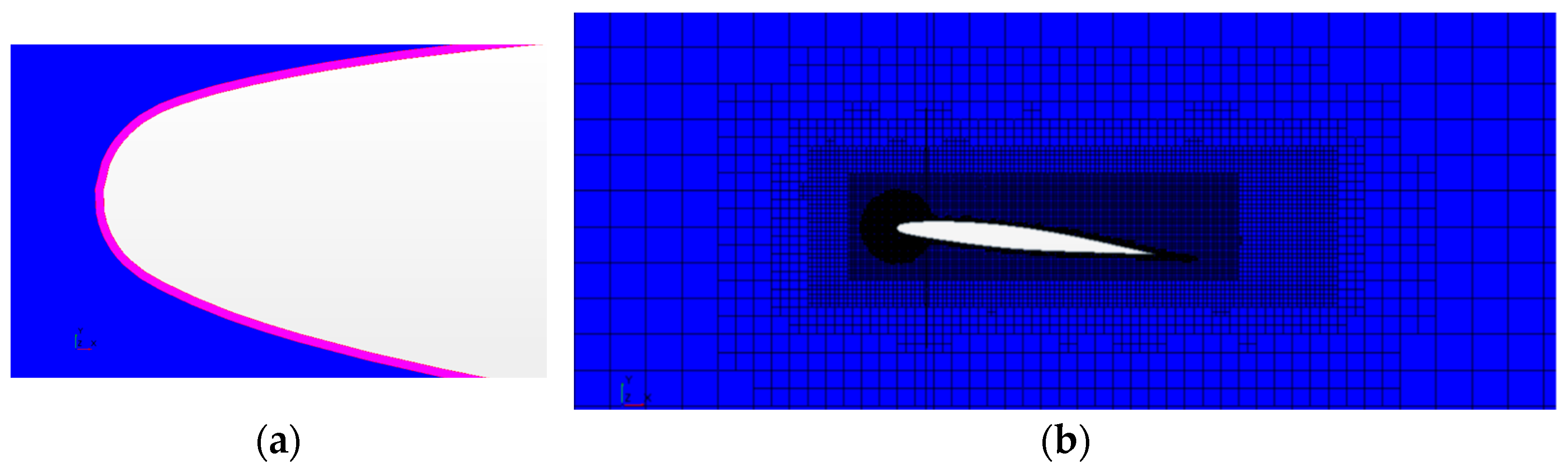
• Morphing: Modify the flow grid (reported in Figure 6b subtracting the solidified ice from the air domain.

The Dispersed Multiphase Model uses equations reported previously for both phases. The approach is identified as “one way”: the external flow can influence the liquid phase through heat and aerodynamic resistance, but the latter cannot influence the gas phase.

The resolution of the fluid film is based on enthalpy. The enthalpy for the liquid solid transition film, ${\mathrm{H}}_{\mathrm{f}}^{*}$ is calculated as follows:

$${\mathrm{H}}_{\mathrm{f}}^{*}{=\mathrm{H}}_{\mathrm{f}}+\left(1-{\mathsf{\alpha }}_{\mathrm{s}}^{*}\right){\mathrm{H}}_{\mathrm{lat}}$$

(10)

where H_f is the sensible enthalpy and $1-{\mathsf{\alpha }}_s^{*}$ represents the portion of the transition film occupied by the liquid phase. ${\mathsf{\alpha }}_s^{*}$ depends on the normalized temperature:

$${\mathsf{\alpha }}_{\mathrm{s}}^{*}=\left\{\begin{array}{c}{1\mathrm{if}\mathrm{T}}^{*}<0\\ \mathrm{f}\left({\mathrm{T}}^{*}\right){\mathrm{if}0<\mathrm{T}}^{*}<1\\ {0\mathrm{if}1<\mathrm{T}}^{*}\end{array}\right.$$

(11)

T* identifies the normalize temperature, evaluated as follows:

$${\mathrm{T}}^{*}=\frac{\mathrm{T}-{\mathrm{T}}_{\mathrm{sol}}}{{\mathrm{T}}_{\mathrm{liq}}-{\mathrm{T}}_{\mathrm{sol}}}$$

(12)

where T_sol represents the solid fraction temperature and T_liq the liquid fraction temperature. Ice thickness growth, represented as ∆h_s, is given by:

$$\mathsf{\Delta }{\mathrm{h}}_{\mathrm{s}}^{\prime }=\left\{\begin{array}{c}-\frac{\mathsf{\Delta }\mathrm{H}\left(\mathrm{T}\right)-\mathsf{\Delta }{\mathrm{H}}_{\mathrm{liq}}}{{\mathrm{H}}_{\mathrm{f}}}(\mathrm{h}+\mathsf{\Delta }{\mathrm{h}}_{\mathrm{s}})\mathrm{if}\mathrm{T}\ge {\mathrm{T}}_{\mathrm{liq}}\\ {\mathrm{h}}_{\mathrm{f}}{\mathsf{\alpha }}_{\mathrm{s}}^{*}\mathrm{if}\mathrm{T}\le {\mathrm{T}}_{\mathrm{liq}}\end{array}\right.$$

(13)

This model does not permit the reduction of the icing formed. It is impossible to simulate the deicing function but only the anti-icing as is.

The magnitude of the ice formed reflects then in the morphing displacement for each phase:

$${\mathrm{d}}_{\mathrm{face}}=\mathrm{K}\mathsf{\Delta }{\mathrm{h}}_{\mathrm{s}}{\mathrm{n}}_{\mathrm{face}}$$

(14)

K is called the solid time step factor. It allows the widening, if necessary, of the displacement magnitude obtaining an acceleration on the simulations.

For all simulations, three-dimensional models have been enabled with an implicit unsteady time step. The type of flow has been selected as a segregated flow and gradients models have been enabled. The equations of the state of ideal gas have been applied for the airflow continuum and the turbulent viscous regime has been modelled with the Reynolds Averaged Navier Stokes. The K-Epsilon turbulence model has been applied.

2.2. Anti Ice Model Setup

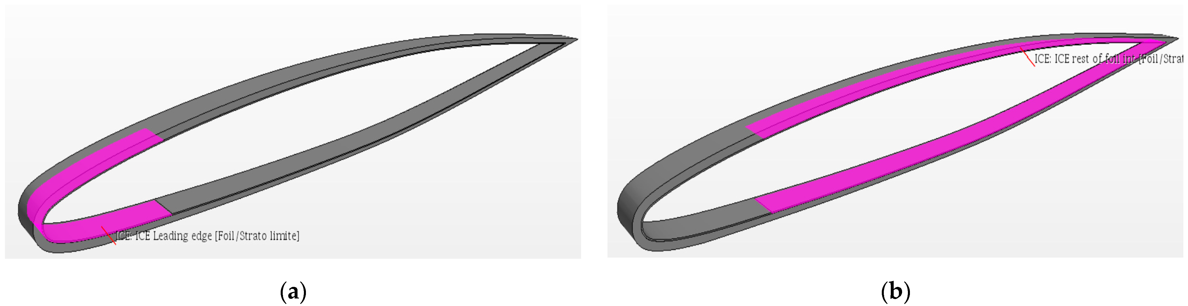
An anti-ice model has been implemented starting from an ice accumulation model and inserting some modifications. A metal solid part has been added, as reported in Figure 6a in purple.

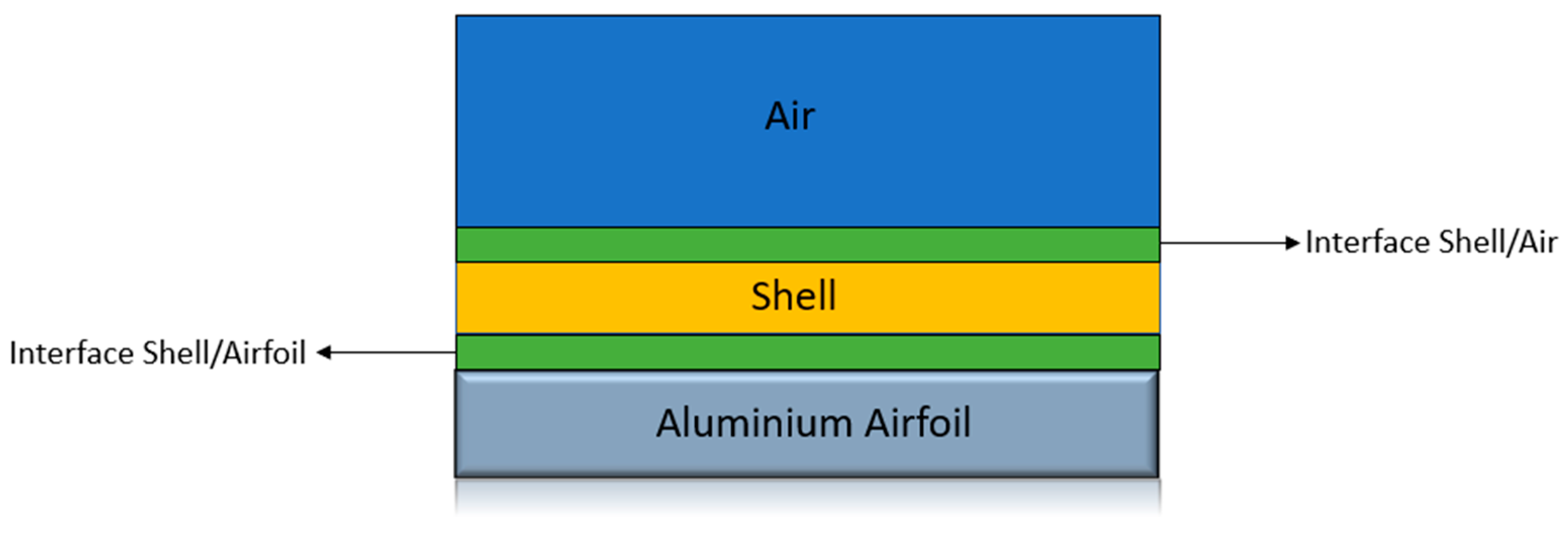
Adding a new metal part requires implementing a new heat exchange interface between the metal profile and the shell with the embedded thin film model. The new schematization is reported in Figure 7.

Two local interfaces between the3D solid mesh and 2D shell mesh requires a perfect and stable correspondence between faces [36]. To permit this correspondence to remain stable and persistent during unsteady calculation as well, the removal of the frozen film thickness has been disabled permanently.

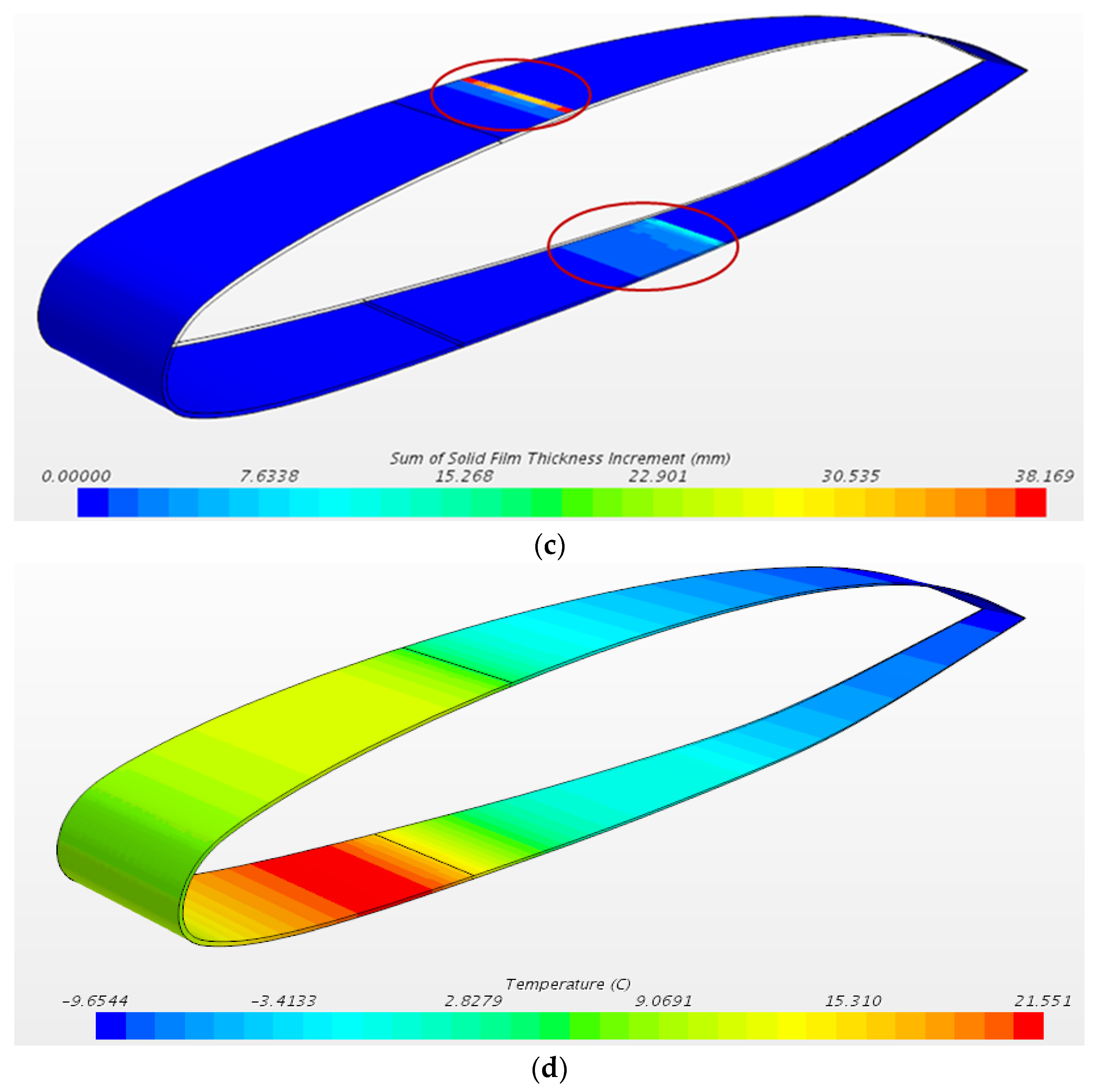
2.3. De Ice Model Setup

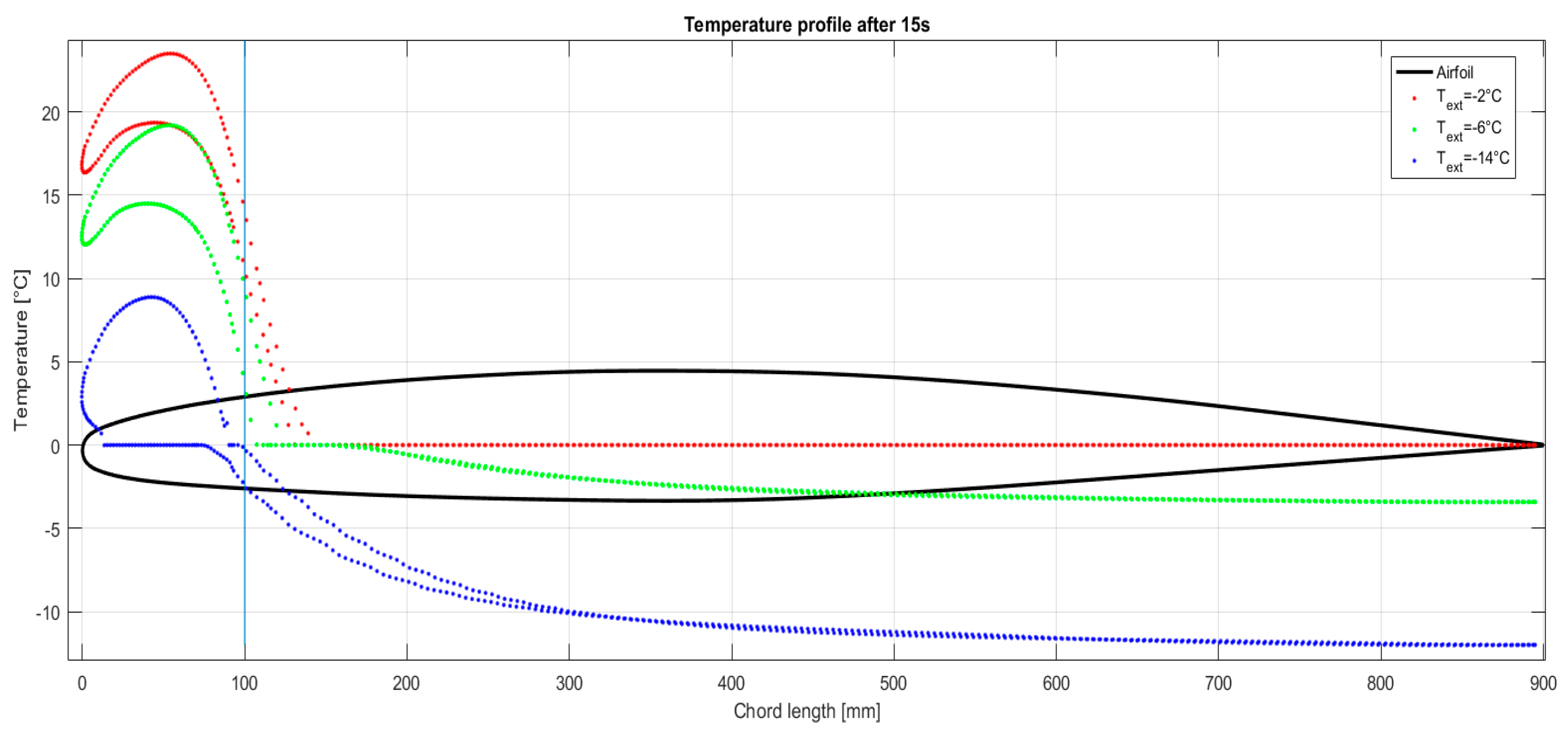
This model aims to evaluate the amount of time necessary to liquefy the ice deposited on the leading edge of the airfoil. Rather than being a deicing for in-flight operation, this tool enables the evaluation of the possibility to remove the ice formed on the airfoil during the pre-flight warm-up. The interest in this feature relies on the possibility of installing the novel anti-ice system on unmanned aerial vehicles (UAV) operated from an airfield with no supporting crew.

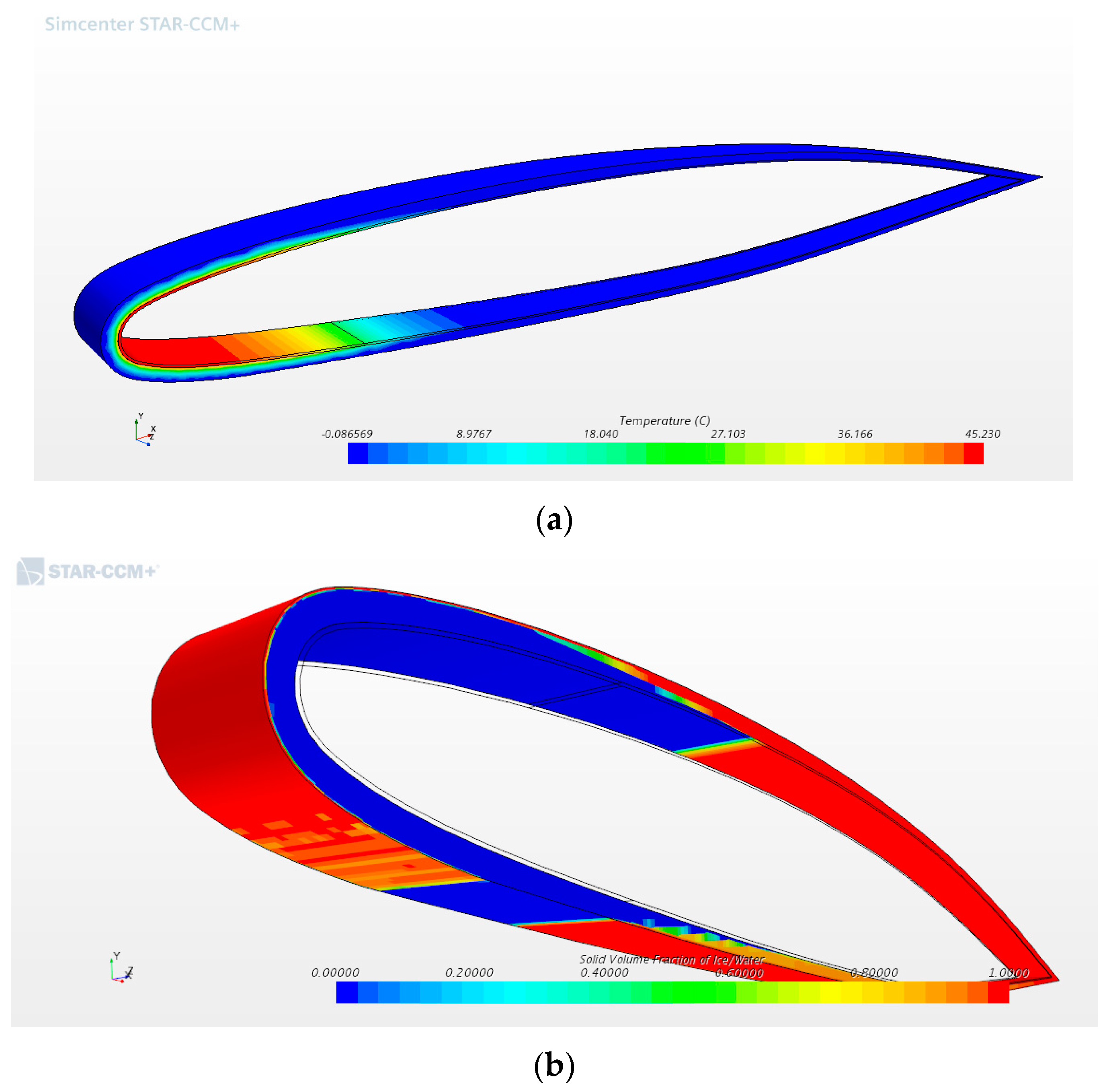
To simulate deicing on the ground, a volume of fluid (VOF) has been adopted. A Eulerian approach has been selected with a thermodynamic solidification and liquefaction model implemented. The material properties of liquid and solid phase are reported in

Table 2. Fluid properties of Liquid and Solid Phases.

	Material Properties
Range Temperature	Density	Thermal Conductivity
T > 273.15 K (Water)	917 kg/m3	0.620 W/mK
T < 273.15 K (Ice)	997 kg/m3	2.330 W/mK

.

The geometric part comprises a metallic airfoil with a superimposed layer of ice with pre-settled thickens. The airfoil has been divided in two parts to simulate the heated leading edge and non-heated back part. A picture of the model is reported in Figure 8.

The advantage of adopting a VOF approach lies in the ease of the access at the concentration of the two phases. It is simple to observe the liquefaction in the front part and the enlargement to the rear half.

3. Results

This section will report the results collected from the model described in Section 2, Materials and Methods. In the first section, the ice accretion model has been validated with NASA TP 2000-210031 Ice Accretion and Icing Effects for Modern Airfoils [9]; in the second section the result obtained for anti-icing will be discussed, and in the third, the result for the deicing function.

3.1. Ice Accretion Model Validation

To validate the ice accretion model, NASA Glenn Research Centre results were used [9]. FAR 25-appendix C (https://www.law.cornell.edu/cfr/text/14/appendix-C_to_part_25) (accessed on 24 March 2023) conditions were considered. A Business Jet airfoil was chosen to be representative due to the similarity with the final application. The section of the profile is reported in Figure 9. This airfoil has been used by the NASA Glenn Research Centre. In this, analysis the same profile, taken by [9], has been adopted. The coordinates are reported in Appendix A (

Table A1. Business Jet Airfoil coordinates.

X/C	Z/C	X/C	Z/C
1.00000	−0.00033	0.00000	−0.00392
0.82500	−0.01321	0.00050	−0.00006
0.80000	−0.01506	0.00100	0.00137
0.77500	−0.01691	0.00150	0.00246
0.75000	−0.01879	0.00200	0.00337
0.72500	−0.02061	0.00300	0.00478
0.70000	−0.02244	0.00400	0.00594
0.67500	−0.02427	0.00500	0.00691
0.65000	−0.02610	0.00750	0.00870
0.62500	−0.02788	0.01000	0.00999
0.60000	−0.02953	0.01250	0.01108
0.57500	−0.03108	0.01500	0.01212
0.55000	−0.03252	0.02000	0.01388
0.52500	−0.03383	0.02500	0.01547
0.50000	−0.03501	0.03000	0.01694
0.47500	−0.03597	0.04000	0.01956
0.45000	−0.03666	0.05000	0.02184
0.42500	−0.03706	0.06000	0.02388
0.40000	−0.03718	0.07500	0.02670
0.37500	−0.03709	0.10000	0.03066
0.35000	−0.03681	0.12500	0.03404
0.32500	−0.03643	0.15000	0.03698
0.30000	−0.03598	0.17500	0.03951
0.27500	−0.03545	0.20000	0.04169
0.25000	−0.03482	0.22500	0.04359
0.22500	−0.03410	0.25000	0.04520
0.20000	−0.03322	0.27500	0.04654
0.17500	−0.03218	0.30000	0.04771
0.15000	−0.03094	0.32500	0.04862
0.12500	−0.02969	0.35000	0.04924
0.10000	−0.02833	0.37500	0.04951
0.07500	−0.02672	0.40000	0.04956
0.06000	−0.02551	0.42500	0.04942
0.05000	−0.02455	0.45000	0.04915
0.04000	−0.02338	0.47500	0.04863
0.03000	−0.02185	0.50000	0.04789
0.02500	−0.02090	0.52500	0.04685
0.02000	−0.01977	0.55000	0.04555
0.01500	−0.01833	0.57500	0.04404
0.01250	−0.01748	0.60000	0.04233
0.01000	−0.01656	0.62500	0.04042
0.00750	−0.01547	0.65000	0.03837
0.00500	−0.01386	0.67500	0.03623
0.00400	−0.01299	0.70000	0.03397
0.00300	−0.01192	0.72500	0.03154
0.00200	−0.01054	0.75000	0.02901
0.00150	−0.00967	0.77500	0.02629
0.00100	−0.00862	0.80000	0.02346
0.00050	−0.00723	0.82500	0.02058
0.00000	−0.00392	1.0	0.00033

. Business Jet Airfoil coordinates).

Five simulations have been used to compare the experimental evidence with the ice accretion simulations obtained by the model evaluation. This simulation differs for external airspeed, temperature, MVD Droplet, LWC, and angle of attack. In this manner, uniform information on the performance of the model can be evaluated representative of different flight conditions and a different icing ambient. The physical properties of the five tests are reported in

Table 3. Model Validation Input Data.

Group	Parameters	Simulations Test Cases
		A	B	C	D	E
External Flow	Velocity [m/s]	129	90	90	90	90
	Temperature [°C]	−20	−15	−18	−18	−18
Dispersed Phase	MVD [µm]	40	20	20	40	40
	LWC [g/m3]	0.41	0.54	0.53	0.53	0.53
Airfoil	AOA	1.5	6.1	6.1	4	6.2
Ice Accretion Time [min]		1.5	6	6	6	6

.

The results collected are graphically reported. The graphs show the experimental ice thickness evaluated by NASA in red and the numerical thickness simulated by the authors is reported with blue dots.

The results computed with the ice accretion model are consistent with the data obtained by NASA. The lower camber line always reports a good correspondence with the experimental points in all tests. The upper camber icing behavior replicates satisfactorily the experimental evidence with the lower accretion time and lower angle of attack at high speed (i.e., Figure 10a). Increasing the angle of attack and reducing the airspeed, it is possible to evidence some underestimation in Figure 10c; the estimation seems to reduce proportionally with the AOA as also reported in Figure 10d. The reason for this phenomena may be in the morphing that reduces the air domain without increasing the surface roughness. Ice formation instead, especially at high AOA, may contribute to the turbulence flow at a microscopical porous level, not possible to simulate with this approach.

Overall, however, the model predictions are consistent with the experimental outcomes in shapes and magnitude in all the tests performed.

3.2. Anti Icing Results

The model, validated in the ice formation and upgraded with the anti-icing feature, has been tested with the conditions of

Table 4. Anti-icing conditions applied.

Group	Parameters	Test Case
External Flow	Velocity [m/s]	90
	Temperature [°C]	−14.75
Dispersed Phase	MVD [µm]	20
	LWC [g/m3]	0.54
Airfoil	AOA	6.1
Ice Accretion Time [min]		1.5
Leading Edge Heat Flux [W/m2]		1 × 104

to evaluate if the heat flux imposed at the leading edge is sufficient for a running wet hypothesis. The airfoil’s initial condition is with no ice attached.

The choice of temperature and speed has been imposed to match with the experimental setup campaign conducted during winter 2022 on aircraft.

Results obtained from the run are reported in Figure 11.

Figure 11a represents the impingement rate, the particles of water that directly contact the surface. Due to the AOA of 6°, the lower camber is the most affected with 0.033 kg/m²·s maximum. The same trend is confirmed by the second image, which reports the thickness of the fluid film, reaching a peak of 0.01mm in the lower camber. Figure 11c confirms that with the heat flux imposed, there is no ice thickness accumulation on the leading edge, providing that the heat flux imposed is sufficient for a running wet anti-icing condition. After half of the chord, the ice tends to accumulate on both the upper and lower profiles in the minor entity. The last image reports evidence of a high temperature on the leading edge (more than 9 °C in the leading edge with a peak of 21.51 °C compared with the external flow temperature of −14.75 °C). The upper profile, spanned by a higher flow velocity, presents a lower temperature compared with the lower profile.

Figure 12 presents the upper and lower temperatures of the airfoil’s external profile, varying the external air temperature. The curves present the same trend, passing from −14 °C (blue) to −6 °C (green) and finally to −2 °C. It is interesting to note that the temperature curve remains unchanged in shape but only gets shifted upwards toward higher temperatures.

3.3. Deicing Results

The deice simulation aims to verify the possibility for the anti-icing system to remove formed ice. This task is intended to verify this possibility for the operation of UAV in airport without human personnel assistance. The same heat flow for anti-icing conditions has been imposed with 5mm ice formed and a simulation time of 7 min. The applied conditions for Deicing are reported in

Table 5. Deicing conditions applied.

Group	Parameters	Test Case
Aluminium	Static Temperature [°C]	−4
	Heat Flux [W/m2]	1 × 104
Ice /Water	Water Density [kg/m3]	997
	Ice Density [kg/m3]	917
	Water thermal conductivity [W/m·K]	0.62
	Ice thermal conductivity [W/m·K]	2.33
	Initial ice layer thickness [mm]	5

.

After 420 s, the temperature at the leading edge is around 58 °C and the ice is liquefying on the correspondent area. Gradually, the rear part is also starting to melt, as evidenced by Figure 13b. These preliminary results reported are cautionary because they do not consider the falling of ice once the layer attaching to the airfoil is liquefied due to vibration and gravity.

4. Conclusions

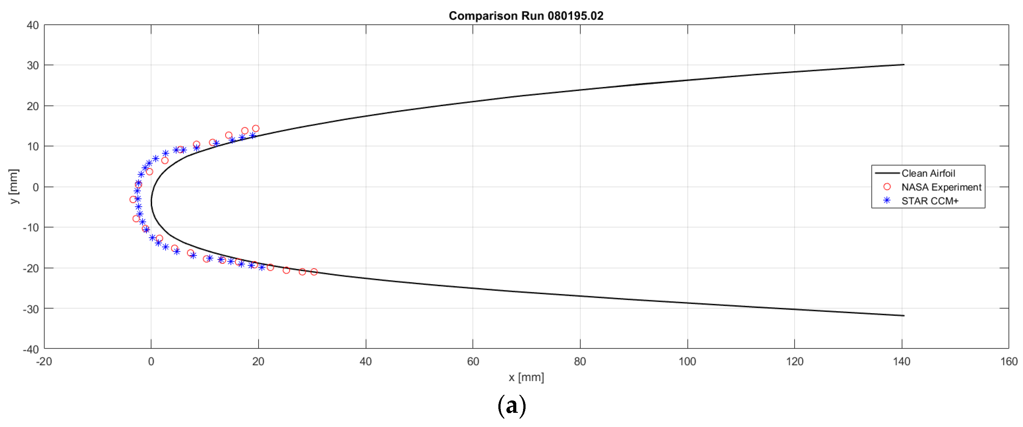
In conclusion, this study has successfully introduced a novel, robust, and validated icing model, aiming to contribute to the field of anti-icing evaluations. Our findings demonstrate that this model can accurately predict quantitative aspects of icing phenomena on airfoils, with the potential for expansion to meet anti-icing demands.

Nonetheless, it is important to acknowledge the inherent limitations present in this investigation. A key constraint is the need for cross-validation with experimental benches, which are currently being developed. This validation is essential to ensure the model’s applicability and reliability when addressing anti-icing requirements. Furthermore, future research should focus on examining the deicing phenomena more closely, as an in-depth understanding of these processes is crucial to enhancing the model’s efficacy and versatility. This comprehensive exploration will not only allow for a more thorough evaluation of the model’s performance but also contribute to the development of innovative and effective solutions to the challenges in aircraft icing.

The implications of this research are far-reaching, with the potential to influence the way aircraft icing is managed and mitigated in the aviation industry. As the model continues to evolve and improve through rigorous research and validation, its impact on enhancing flight safety and efficiency will become increasingly apparent. This study represents a notable step in the ongoing quest for advanced and reliable anti-icing strategies, emphasizing the vital role of scientific innovation and collaboration in pursuing safer skies for all.

5. Patents

This work is part of the development of the patent of a novel anti-icing system for aircraft use [24].