Article

Physics-Informed Neural Network for Flow Prediction Based on Flow Visualization in Bridge Engineering

1
Zhejiang University-University of Illinois at Urbana-Champaign Institute, Zhejiang University, Haining 314499, China
2
School of Aeronautics and Astronautics, Zhejiang University, Hangzhou 310013, China
3
School of Advanced Technology, Department of Mechatronics and Robotics, Xi’an Jiaotong-Liverpool University (SIP Campus), Suzhou 215000, China
*
Author to whom correspondence should be addressed.
These authors contributed equally to this work.
Atmosphere 2023, 14(4), 759; https://doi.org/10.3390/atmos14040759
Submission received: 17 February 2023 / Revised: 6 April 2023 / Accepted: 17 April 2023 / Published: 21 April 2023
(This article belongs to the Section Atmospheric Techniques, Instruments, and Modeling)

Abstract

:
Wind loads can endanger the safety and stability of bridges, especially long-span cable-supported bridges. Therefore, it is important to evaluate the potential wind loads during the bridge design stage. Traditionally, wind load evaluation is performed by wind tunnel testing, which is relatively expensive. With the development of computational fluid dynamics and high-performance computing, numerical simulations are becoming more accessible for designers. However, the costs required for accurate numerical results are still high, especially for high-fidelity simulations. Under this condition, searching for a more efficient method to evaluate the wind loads in bridge wind engineering has become a new goal. It seems that flow visualization is a good entry point. Although flow visualization techniques have been developed in recent years, it remains difficult to extract velocity and pressure fields from images. To address this problem, physics-informed neural networks (PINNs) have been developed and validated. This study establishes a PINN to investigate the two-dimensional viscous incompressible fluid flow passing a generic bridge deck section. Two cases with different Reynolds numbers are tested. After careful training, it is found that the PINN can accurately extract the velocity and pressure fields from the concentration field and predict the drag and lift coefficients. The results demonstrate that PINNs are a promising method for extracting useful flow information from flow visualization data in engineering applications.

1. Introduction

Wind loads are an important design consideration for bridges, especially long-span cable-supported bridges [1]. If the wind loads are not properly constrained, the bridge lifecycles can be greatly reduced. Traditionally, wind load data are obtained from wind tunnel tests [2,3]. Wu et al. [4] studied the nonlinear characteristics of bridge motion under wind loads through wind tunnel testing, while Xin et al. [5] investigated the static characteristics of bridges under wind and rain loading through a series of experiments. Kwon et al. [6] investigated the effects of wind on suspension bridge catwalks, and Diana et al. [7] performed wind tunnel tests on a long-span suspension bridge. However, wind tunnels have long construction periods and are expensive to build.
In recent years, computational fluid dynamics (CFD) has been applied to the analysis of wind loads on bridges [8,9,10]. However, CFD simulations require substantial computing resources, especially for three-dimensional high-fidelity simulations. With the development of central processing units and distributed computing, CFD and deep learning have improved significantly. Deep learning was first used to solve ordinary and partial differential equations in the 1990s [11]. However, its development and application were hampered by limitations on computational resources, and the corresponding research did not receive much attention. In the past three decades, with the development of computer science and engineering, high-performance computational power has become easily accessible to both the research and design communities. This has contributed to the development of artificial intelligence (AI). With the rapid progress of AI, deep learning has been increasingly applied in fluid mechanics [12]. Raissi et al. [13,14] revived the idea of physics-informed neural networks (PINNs) in 2019 to solve forward and inverse nonlinear physical problems. In recent years, PINNs have gradually attracted the attention of many researchers. Mathematically speaking, a neural network can be treated as a function approximator. The process of training a model is similar to the process of seeking a solution that satisfies a given constraint. Therefore, we can embed the physical laws into neural networks through loss functions. Hence, we can obtain solutions to equations by minimizing the loss functions.
Over the past few years, PINNs have been developed and improved for various applications and specific problems. For example, Fang et al. [15] studied higher-order nonlinear Schrödinger equations using a PINN, while Chen et al. [16] developed a PINN to investigate the water-wave-based Korteweg–de-Vries equation. Meng et al. [17] proposed a parallel PINN model that transforms a long-time problem into multiple short-time problems. They found that the parallel PINN model significantly improves the convergence speed. A conservative PINN model was proposed by Jagtap et al. [18], who divided the computational domain into multiple subdomains and added flux conservation laws in adjacent subdomains as a boundary condition to the loss function.
PINNs can be divided into two types, namely data-driven and non-data-driven models. For the former, Raissi et al. [13,14] introduced a PINN model with the capacity to approximate partial differential equations. This has been widely used to achieve better performance in fluid mechanics applications, where the neural network learns a surrogate mapping between input and output. Kissas et al. [19] used a PINN to model arterial blood pressure with magnetic resonance imaging data and physical laws, and Raissi et al. [20] proposed a PINN model that extracts velocity and pressure fields from flow visualizations. In terms of non-data-driven models, Sun et al. [21] constructed an unsupervised PINN model for simulating fluid flows. Zhu et al. [22] proposed a physics-informed convolutional encoder–decoder unsupervised neural network to model fluid flows, while Rao et al. [23] introduced the Cauchy stress tensor into the Navier–Stokes equation within a neural network environment to improve the convergence. However, compared with data-driven models, non-data-driven PINNs offer poor convergence, especially for problems over long timescales. Moreover, there has been little research on PINNs for obtaining the velocity and pressure fields in bridge engineering applications.
This paper describes a data-driven PINN model that extracts the velocity and pressure fields from the concentration field and applies it in bridge engineering for obtaining the velocity and pressure from the concentration field (e.g., a smoke field). The remainder of this paper is organized as follows. Section 2 introduces the principles and purpose of the PINN model. Section 3 then presents the geometry and corresponding boundary/initial conditions, before Section 4 describes a comparison study that demonstrates the feasibility of extracting the flow field from flow visualization. Finally, Section 5 summarizes the conclusions that can be drawn from the comparison study.

2. Methodology

Usually, for Newtonian fluids, the dynamic properties of the fluid are described by the Navier–Stokes equations. These equations describe the actual dynamics of any fluid flows, such as ocean currents, pipe flows, air flows around bridges, and blood flows. The momentum conservation equations are given in Equations (1) and (2). For incompressible fluids, an additional equation is needed to jointly describe the fluid motion. This is the continuity equation (shown in Equation (3)), which describes the conservation of mass of the fluid. To describe the transport of the passive scalar with the fluid motion, we use a transport equation for the passive scalar, which is given in Equation (4).
u t + u u x + v u y + p ρ x - υ 2 u x 2 + 2 u y 2 = 0
v t + u v x + v v y + p ρ y - υ 2 v x 2 + 2 v y 2 = 0
u x + v y = 0
c t + u c x + v c y - λ 2 c x 2 + 2 c y 2 = 0
M S E v p , v o = i = 1 N v p , i - v o , i 2 N
l o s s d a t a s e t = M S E c p r e d , c t r u e
l o s s p h y s i c s = l o s s N S X + l o s s N S Y + l o s s c o n t i n u i t y + l o s s c o n c e n t r a t i o n
l o s s N S X = M S E 0 , u t + u u x + v u y + p ρ x - ν 2 u x 2 + 2 u y 2
l o s s N S Y = M S E 0 , v t + u v x + v v y + p ρ y - ν 2 v x 2 + 2 v y 2
l o s s c o n t i n u i t y = M S E 0 , u x + v y
l o s s c o n c e n t r a t i o n = M S E 0 , c t + u c x + v c y - λ 2 c x 2 + 2 c y 2
l o s s = l o s s d a t a s e t + l o s s p h y s i c s
where p is the pressure; u , v are the velocity components in the horizontal and vertical directions, respectively; υ is the kinematic viscosity; ρ is the density of the fluid; c is the concentration of the passive scalar; λ is the mass diffusion coefficient; v p , i is the predicted output data at point i; v o , i is the original data at point i; N is the number of sampling points.
For the purpose of extracting the velocity and pressure fields, a PINN model is used. A schematic of this model is shown in Figure 1. The PINN model is derived from a multilayer perceptron (MLP). Usually, MLPs are used to map the input and output values in a certain dataset, and the mean square error (MSE) is used to construct the loss function between the predicted output data and the original data, as defined in Equation (5). In this PINN model, the concentration field is taken as the training data, and its loss function is denoted as l o s s d a t a s e t (shown in Equation (6)). This is the MSE between the predicted and original concentration fields of the passive scalar. To fit some physical phenomena using the neural network, we embed the governing equations into the loss function. We can then denote these loss functions as l o s s p h y s i c s (shown in Equation (7)) and the neural network becomes a PINN. l o s s p h y s i c s is the MSE between the left and right ends of the governing equations, including l o s s N S X , l o s s N S Y , l o s s c o n t i n u i t y , and l o s s c o n c e n t r a t i o n (shown in Equations (8)–(11)). These represent the embedded momentum conservation equations, continuity equation, and transport equation, respectively, and the loss is the sum of l o s s d a t a s e t and l o s s p h y s i c s (shown in Equation (12)).
Automatic differentiation is used in the PINN model to construct l o s s p h y s i c s . This has been applied in many fields, including statistical inference [24], physics simulations [25], and optimal control [26]. The automatic differentiation technique is different from numerical differentiation and symbolic differentiation. In automatic differentiation, all numerical operations are considered as a finite set of elementary meta-operations. The final differential value can be obtained by integrating these elementary meta-operations and their differential value. The calculation is based on the accurate chain rule for the derivation of composite functions.
Usually, deep learning frameworks have built-in automatic differentiation. The process of training the model involves minimizing the loss (as shown in Figure 1). The minimization is based on an optimization algorithm, such as Adam [27], LBFGS [28], SGD [29], and their variants, e.g., AdamW, RAdam, NAdam, Adadelta, Adagrad, SparseAdam, ASGD, Rprop, and RMSprop. These optimization algorithms are essentially gradient descent methods based on automatic differentiation. Different frameworks such as TensorFlow [30], Pytorch [31], Jax, and PaddlePaddle are also available. In Pytorch, the computational graph is dynamically defined, whereas in TensorFlow 1.x, it is statically defined, and dynamic graphs are used in 2.x because of the unique advantages of dynamic graphs. The static graphs framework means that the developer needs to define the computational graph first and then use it constantly, while the dynamic graphs framework rebuilds a new computational graph each time. Dynamic computation means that the program will execute in the order in which the developers write the commands. This mechanism makes debugging easier and simplifies the translation of ideas into actual code. Static computation means that the graph is generated once and used repeatedly. The graph does not need to be reconstructed as the code is running, so this approach is theoretically faster than using dynamic graphs. Static computation also allows for greater optimization by the compiler, but makes human–computer interaction and debugging activity more difficult.
Flow visualization is the art of visualizing flow patterns. There are two main different means of flow visualization, one is experimental and the other is theoretical [32,33,34]. For experimental means, there are currently three main visualization methods, namely surface flow visualization, the particle tracer method, and the optical method. For the theoretical means, there are currently two main visualization methods, the analytical methods and the textural advection methods.
In bridge engineering, we can easily obtain a concentration field by particle tracer methods or optical methods, but the velocity and pressure fields are not easily obtained directly. In this work, the architecture of the PINN for fluid dynamics (shown in Figure 1) is implemented using Pytorch [31] and is used to obtain the velocity and pressure fields from the concentration field. The transport equation of the passive scalar is embedded into this model. We must emphasize that in the model, the concentration field is the only input data and it can be obtained by the flow visualization method, and the velocity and pressure fields are the data we want to obtain through the model; hence, the title of this paper includes Flow Prediction Based on Flow Visualization.
In this study, a high-resolution concentration dataset is generated through Nektar++, an open-source CFD solver based on the spectral/hp element algorithm [35,36,37]. Nektar++ approximates the Navier–Stokes and transport equations using high-order semi-orthogonal Jacobian polynomial expansions [38]. After constructing the PINN model, we extract the velocity and pressure fields by flow visualization. In the training process, the geometry, boundary conditions, and initial conditions are not necessary. However, if the boundary conditions are given, the trainability and training speed will be improved. We obtain the concentration field through numerical simulations.
It is possible that, in the future, a PINN model could be introduced to predict the flow field from experimental data. This idea still needs to be verified by experiments such as wind tunnel tests. We could then use a concentration detector to detect and record the corresponding concentration data. After obtaining the measured concentration field, the flow field could be extracted from the measured data using a PINN.

3. Geometry and Boundary Conditions

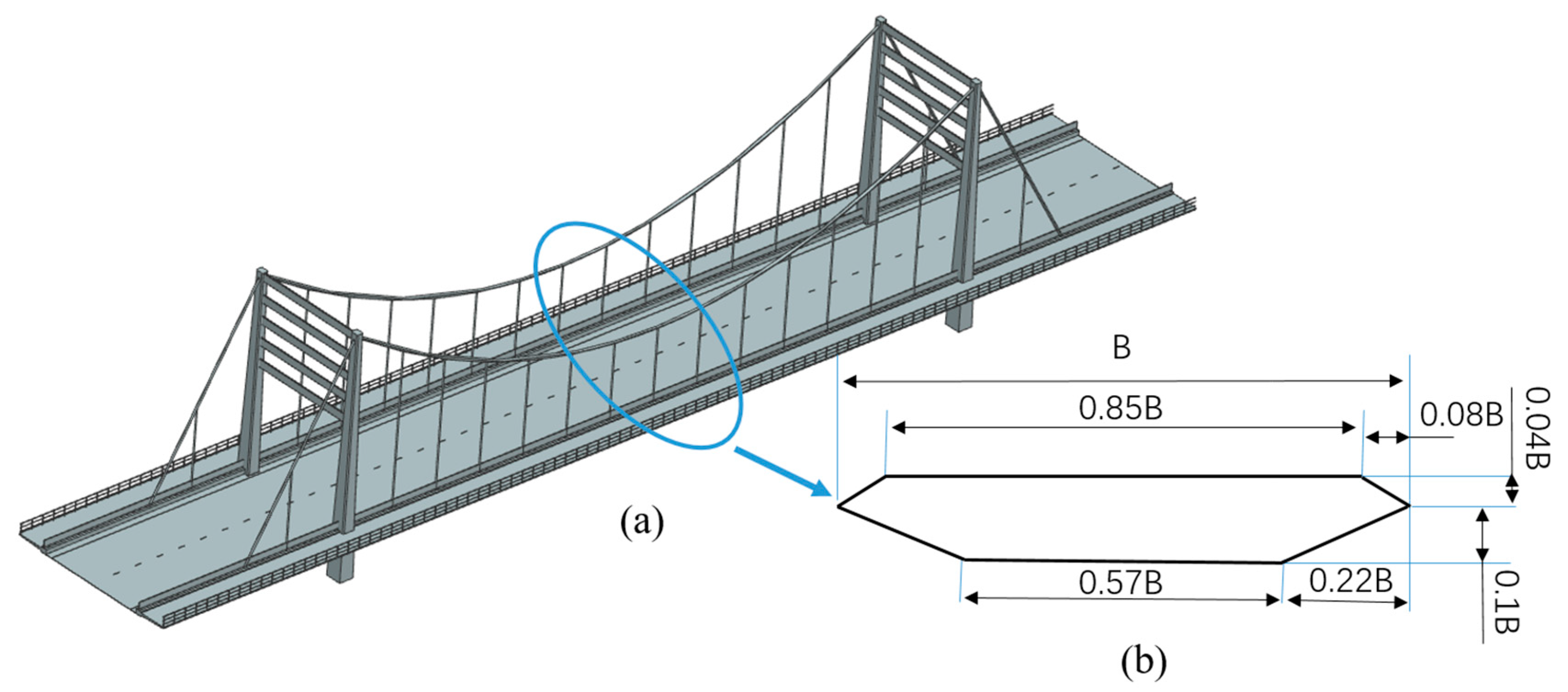
The vortex-induced vibrations of the wind field have the potential to damage bridges, especially long-span bridges [39,40,41]. A typical example is the Humen Bridge in China. Significant vibrations occur in this bridge under the vortex-induced vibration effect. The profile of the bridge deck section has an impact on this effect. Thus, it is necessary to investigate the flow field around the bridge deck section. To examine the effect caused by this wind field, Scanlan et al. [42] studied five generic deck sections, including four block sections and one H-section. As they obtained similar results for all five geometries, only a single geometry is used in the present study. The geometric dimensions considered herein are shown in Figure 2, and the computational domain is shown in Figure 3a.
We use the open-source spectral/hp element solver Nektar++. The mesh distribution, shown in Figure 3b, has refinements in certain areas to obtain more accurate results. The meshing tool used in this study is gmesh. To obtain the determined flow field, the initial and boundary conditions must be given. As Figure 3a shows, the inlet left boundary, outlet right boundary, and top/bottom boundaries are assigned periodic boundary conditions. The geometry is set to have 0-Dirichlet boundary conditions for velocity components and concentration, and 0-Neumann boundary conditions for pressure. The inlet is set to have 1-Dirichlet boundary conditions in the u component and concentration, 0-Dirchlet boundary conditions in the v component, and 0-Neumann boundary conditions in the pressure. The outlet is set to have 0-Neumann boundary conditions in the u and v components and concentration, and 0-Dirichlet boundary conditions in the pressure (here, the 0-Dirichlet/Neumann boundary condition means that the value/gradient of velocity or pressure is 0; the 1-Dirichlet boundary condition is used for the u component at the inlet, which means that UB = 1 at the inlet; that is, if we take the value of both u and B as 1, then the Reynolds number R e = 1 / υ and the Peclet number P e = 1 / λ , and then we can control the Reynolds/Peclet number in our case just by adjusting the viscosity/diffusion coefficient). In the cases studied herein, the global mesh size is 0.075B, with a refined mesh of 0.025B near the deck section and a refined mesh of 0.0375B near the wave zone.
After generating the mesh and setting the boundary conditions, we can obtain the velocity field, pressure field, and concentration field. The concentration field is taken as the input to the PINN while the velocity and pressure fields provide a reference for the PINN output.

4. Results

4.1. Dataset

We simulate 50 dimensionless time units, as defined in Equation (15), for the Re = 1250 case and 30 dimensionless time units for the Re = 5000 case. Increments of Δ T = 0.001 are adopted throughout the simulations.
R e = U B υ
P e = U B λ
T = t U B
where B is the characteristic length (see Figure 2); U is the flow speed of fluid; R e is the Reynolds number; P e is the Peclet number; t is time.
After generating the mesh and setting the boundary conditions, we assign the parameters (see Table 1) and run the CFD solver. The training data are illustrated in Figure 4 and Figure 5. Using 16 CPU cores, the CFD method takes roughly 180 min and 120 min for cases 1 and 2, respectively.

4.2. Flow Field Prediction

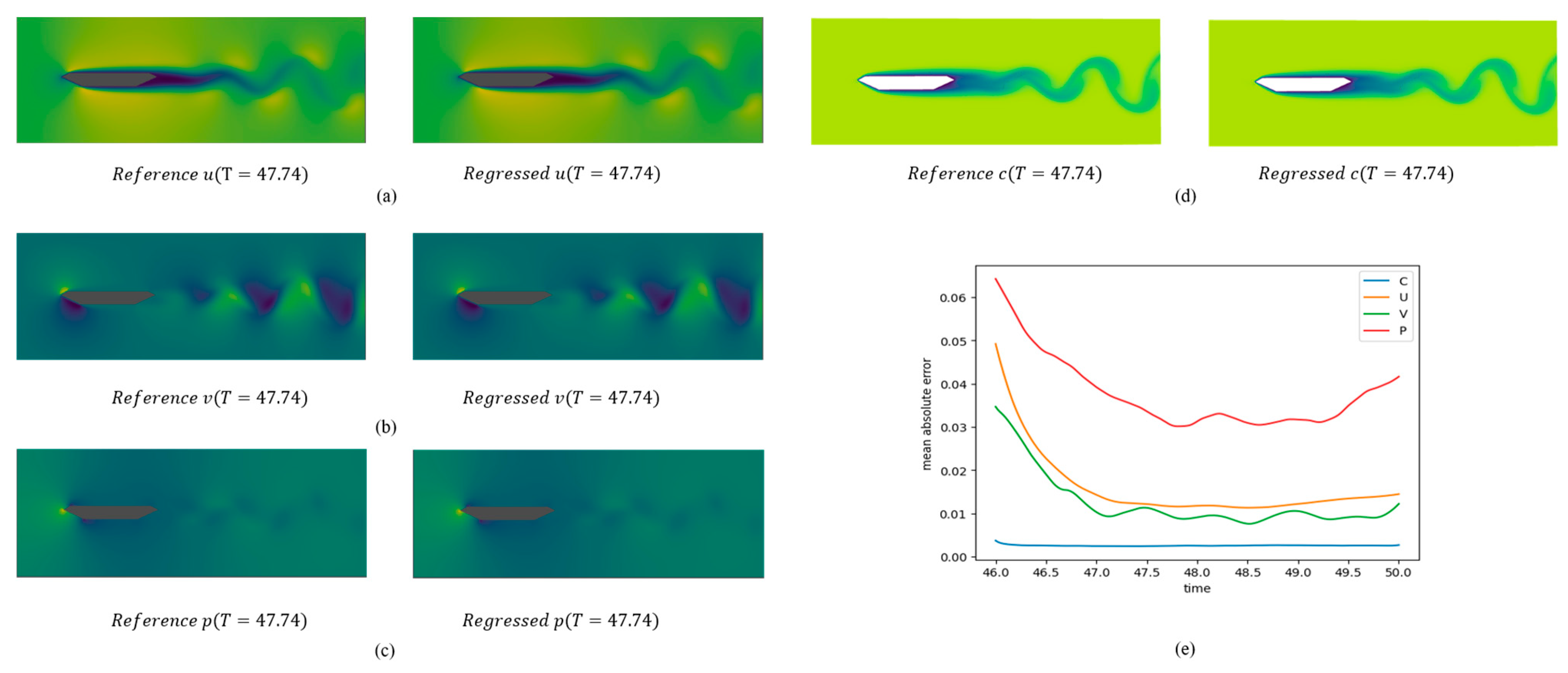
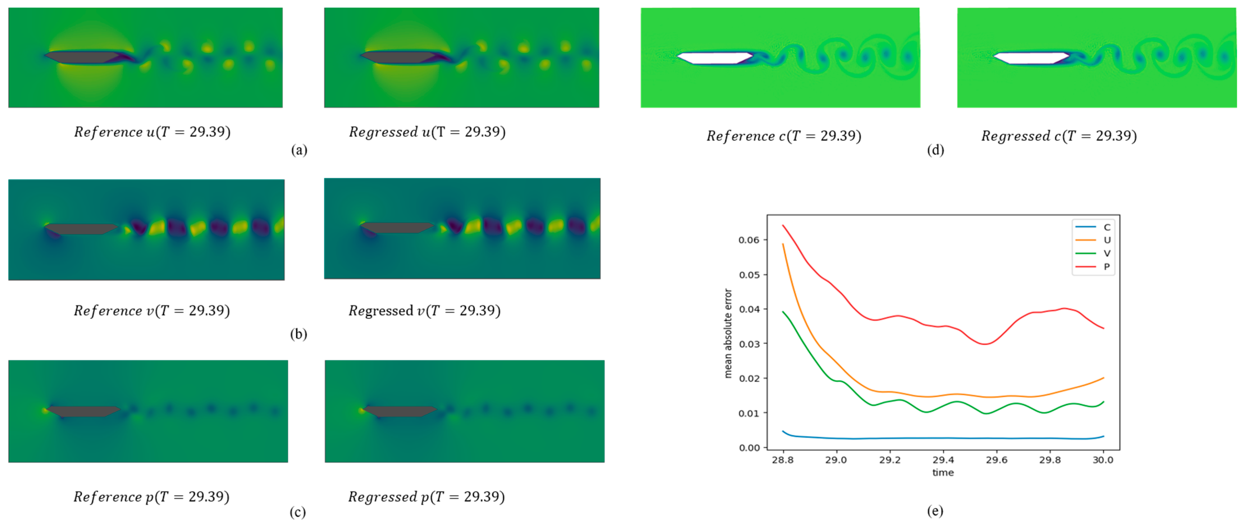
Figure 4 shows the concentration field for Re = 1250. The passive scalar flows from the inlet on the left and flows with the fluid to the outlet on the right at T = 4. However, the concentration field is not stable until T = 25. Thus, the concentration field from T = 46–50 is taken as the training data, as shown in Figure 4a, from which distinct vortices and periodicity can be observed. Similar to Figure 4, Figure 5 shows the concentration field obtained by the CFD solver for Re = 5000. The passive scalar flows to the outlet on the right at T = 4 and reaches a stable state at the same time. The vortex shedding period is roughly double that for the first case. The concentration field from T = 28.8–30 is taken as the training data, as shown in Figure 5a.
The velocity and pressure fields are then learned from the concentration field by the PINN, in which the Adam optimizer is used to train the neural network. After setting the hyperparameters (see Table 2) and training the network, the velocity and pressure fields are predicted based on the concentration field.
To measure the accuracy of the predicted results, we use the MAE (Mean Absolute Error) ϵ , defined as
ϵ = i = 1 N | ξ p , i   -   ξ o , i | N
where ξ denotes the variables u , v , c , p ; ξ p denotes the predicted value by PINN; ξ o denotes the predicted value by CFD.
Figure 6 and Figure 7 compare the predicted data with the reference data at Re = 1250 and Re = 5000, respectively. The datasets are clearly in good agreement, with both the number and shape of the vortices being the same. The MAE between the predicted data and reference data at different Reynolds numbers is given in Figure 6e and Figure 7e. For case one, the max ϵ occurs in p and is 0.0375 (shown in Table 3), and the percentage form is 3.36% (shown in Table 4); for case two, the max ϵ occurs in p and is 0.0394 (shown in Table 3), and the percentage form is 2.76% (shown in Table 5). The max error is no more than 5%, so we can infer that the PINN extracts the velocity and pressure field from the concentration field accurately. Thus, the results obtained by this PINN are good. The comparisons in Figure 6a–c and Figure 7a–c indicate that the PINN accurately reconstructs the velocity and pressure fields, too. Moreover, the error is lower in the middle part and higher at the two ends. This is because of the lack of data before the initial point and after the final point. Thus, this should be taken into consideration when inference is required within a certain time interval.

4.3. Prediction of Drag and Lift Coefficients

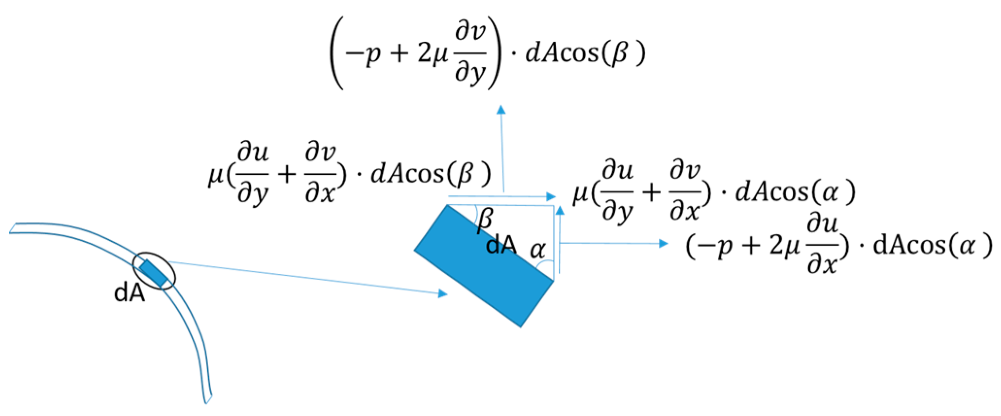
In bridge engineering, we are interested in the drag and lift. On the bridge surface, the aerodynamic forces (lift and drag) contain two main components, one caused by the normal pressure and the other by the tangential viscous force. They can be expressed in terms of a stress tensor σ , which, for the two-dimensional case, contains two normal components and two tangential components, and in the Cartesian coordinate system, the stress tensor is given by
σ = σ x x   σ x y σ y x   σ y y
where the elements in the diagonal σ i i indicate the normal stress; σ i i < 0 means under pressure and σ i i > 0 means under tension. The element σ i j in the non-diagonal line indicates the tangential stress.
To further investigate the composition of the stress, σ can also be split into two parts, as in Equation (18).
σ = - p I + τ
where I is the identity tensor, τ is the viscous stress tensor, and p is the dynamic pressure that occurs in Navier–Stokes equations. It equals the negative value of the average of the three normal stresses, as in Equation (19).
p = 1 2 σ x x + σ y y
For a Newtonian fluid, τ can be expanded into Equation (20).
τ = 2 μ u x + γ · v μ u y + v x μ u y + v x   2 μ u x + γ · v
where γ is the bulk viscosity coefficient, which is usually treated as equal to - ( 2 / 3 ) μ ; · v denotes the divergence of velocity, whose value is equal to 0 for incompressible fluids, so in this paper, τ is given by
τ = 2 μ u x   μ u y + v x μ u y + v x   2 μ u x
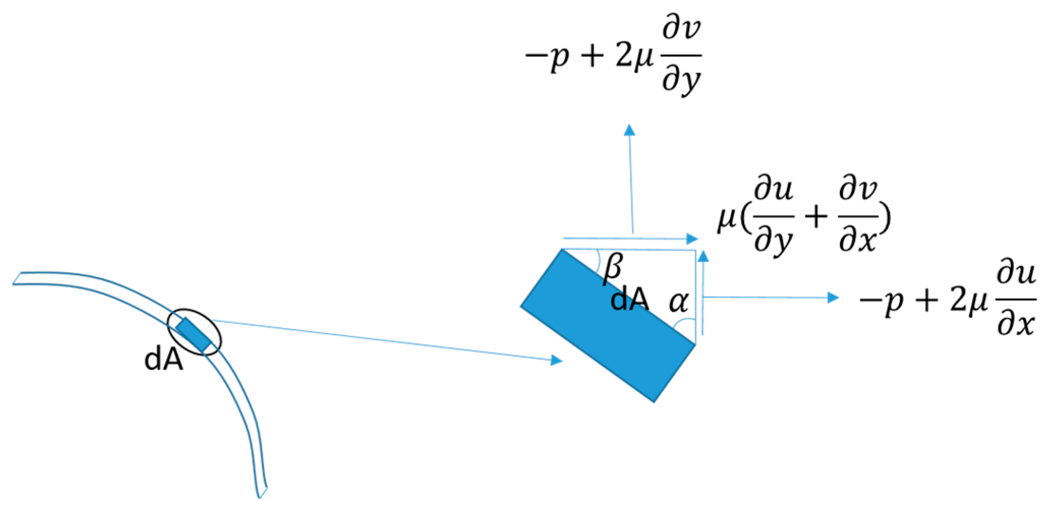
At this point, we can calculate the lift and drag forces, first considering the micro-element as shown in Figure 8.
A micro-element on the surface of the geometry is taken for the analysis in the figure, giving the components of the area of the micro-element in the horizontal and vertical directions, where n denotes the unit normal vector in the surface of the geometry; α and β are the angles between the normal direction and the horizontal and vertical directions, respectively; A denotes the surface geometry.
In order to obtain the lift and drag forces, we also need to know the distribution of the total stresses in the horizontal and vertical directions. So, we next label the total stress given by Equation (18), as shown in Figure 9.
Next, we multiply the stress and the corresponding area of the micro-element to obtain the lift and drag forces on the micro-element, and then integrate them over the entire geometry surface to obtain the lift and drag forces (as Figure 10 and Equations (22) and (23) show).
D = A p + 2 μ u x cos α + μ u y + v x cos β d A
L = A - p + 2 μ v y cos β + μ u y + v x cos α d A
We can obtain the differential values directly from the trained model, but integral values cannot be calculated by a computer directly. So, we have to convert the above equation into a discrete summation over the geometric surface as shown in Equations (24) and (25). Then, the drag coefficient is given by Equation (26) and the lift coefficient is given by Equation (27).
D = i = 0 N e - p i + 2 μ u i x cos α i + μ u i y + v i x cos β i A
L = i = 0 N e - p i + 2 μ v i y cos β i + μ u i y + v i x cos α i A
C d = 2 D ρ U 2 B
C l = 2 L ρ U 2 B
where μ denotes the dynamic viscosity, D denotes the drag, and L denotes the lift.
It is noteworthy that in the calculation of lift and drag, the differential values are obtained by PINNs, while the integral values are solved by discretization of the geometric surface. The former does not involve discrete errors, while the latter involves discrete errors. The results obtained by the PINN method are shown in Figure 11 and Figure 12 and are compared with the results obtained by the CFD method at both Reynolds numbers 1250 and 5000. It can be seen that the results of both agree well, both in terms of amplitude and frequency. Some variations in the error can be observed in Figure 11 and Figure 12. It can be seen that the error is smaller in the middle and larger at the ends, although it is not obvious enough, and this trend is close to the variations in the MAE error in Figure 6 and Figure 7. There are many reasons for the error, probably because the model is stuck at a certain stationary point during training and only finds a local optimal solution, but not the global optimal solution. The error size is not same when using different optimizers or activation functions, the optimizer used in this paper is a combination of Adam and LBFGS, and the activation function is tanh. How different optimizers or activation functions affect the error is unknown and needs to be explored. As for the distribution of errors that are larger in the middle and smaller at the ends, we guess that sufficiently accurate predictions are based on sufficient training data. For example, if we want to predict the velocity and pressure at x = y = t = 1, then we need data within the range of (0, 2) for x, y, and t. That means that if the provided concentration field contains the range of (0, 2) for x, y, and t, then we can obtain a more accurate result, and vice versa, the error will be bigger. For this guess, more research is needed to verify the veracity.

5. Conclusions

This paper has described the use of a PINN to extract the velocity and pressure fields from the concentration field in bridge wind engineering. Two cases are considered, namely fluid flow past a generic bridge deck at Re = Pe = 1250 and Re = Pe = 5000. After training the network, the PINN model successfully reconstructs the flow field of these two cases. The accuracy of the predicted flow field is evaluated in terms of the mean absolute error.
The results obtained in this study indicate that the PINN model can construct and provide a high-fidelity flow field. In particular, the PINN model correctly predicts the drag and lift coefficients. The proposed PINN accurately extracts the velocity and pressure fields from the concentration field and calculates the lift and drag forces. Thus, the results presented in this paper provide a means whereby bridge engineering studies can obtain the flow field through flow visualization. It is believed that similar PINN models could be introduced to solve other bridge engineering problems in the future.

Author Contributions

Conceptualization, H.Y.; methodology, H.Y. and Y.W.; software, H.Y.; formal analysis, H.Y. and Y.W.; investigation, H.Y. and J.C.; resources, H.Y.; data curation, H.Y.; writing—original draft preparation, H.Y.; writing—review and editing, H.Y., Y.W., and J.C.; visualization, H.Y.; supervision, J.C. and Y.Y.; project administration, J.C. and Y.Y.; funding acquisition, J.C. All authors have read and agreed to the published version of the manuscript.

Funding

This study was supported in part by the Zhejiang University/University of Illinois at Urbana-Champaign Institute and the National Natural Science Foundation of China (Grant Nos. 52106060 and 92152202).

Institutional Review Board Statement

Not applicable.

Informed Consent Statement

Not applicable.

Data Availability Statement

The data that support the findings of this study are available from the corresponding author upon reasonable request.

Conflicts of Interest

The authors declare no conflict of interest.

References

  1. Yang, Y.; Fahmy, M.F.; Guan, S.; Pan, Z.; Zhan, Y.; Zhao, T. Properties and applications of FRP cable on long-span cable-supported bridges: A review. Compos. Part B Eng. 2020, 190, 107934. [Google Scholar] [CrossRef]
  2. Liu, Q.K. Aerodynamic and structure design of multifunction boundary-layer wind tunnel. J. Exp. Fluid Mech. 2011, 25, 66. [Google Scholar]
  3. Suzuki, M.; Tanemoto, K.; Maeda, T. Aerodynamic characteristics of train/vehicles under cross winds. J. Wind Eng. Ind. Aerodyn. 2003, 91, 209. [Google Scholar] [CrossRef]
  4. Wu, T.; Kareem, A. Aerodynamics and aeroelasticity of cable-supported bridges: Identification of nonlinear features. J. Eng. Mech. 2013, 139, 1886. [Google Scholar] [CrossRef]
  5. Xin, D.; Li, H.; Wang, L.; Ou, J. Experimental study on static characteristics of the bridge deck section under simultaneous actions of wind and rain. J. Wind Eng. Ind. Aerodyn. 2012, 107, 17. [Google Scholar] [CrossRef]
  6. Kwon, S.D.; Lee, H.; Lee, S.; Kim, J. Mitigating the effects of wind on suspension bridge catwalks. J. Bridge Eng. 2013, 18, 624. [Google Scholar] [CrossRef]
  7. Diana, G.; Rocchi, D.; Belloli, M. Wind tunnel: A fundamental tool for long-span bridge design. Struct. Infrastruct. Eng. 2015, 11, 533. [Google Scholar] [CrossRef]
  8. Hur, N.; Kim, S.R.; Won, C.S.; Choi, C.K. Wind load simulation for high-speed train stations. J. Wind Eng. Ind. Aerodyn. 2008, 96, 2042. [Google Scholar] [CrossRef]
  9. Ding, Y.; Zhou, S.X.; Wei, Y.Q.; Yang, T.L.; Dong, J.L. Influence of wind speed, wind direction and turbulence model for bridge hanger: A case study. Symmetry 2021, 13, 1633. [Google Scholar] [CrossRef]
  10. Zhang, Z.; Zhang, X.; Chen, Z. Status of the application of turbulence models in CFD simulations of bridge aerodynamic load. Eng. Mech. 2016, 33, 1–8. [Google Scholar]
  11. Lagaris, I.; Likas, A.; Fotiadis, D. Artificial neural networks for solving ordinary and partial differential equations. IEEE Trans. Neural Netw. 1998, 9, 987–1000. [Google Scholar] [CrossRef] [PubMed]
  12. Kutz, J.N. Deep learning in fluid dynamics. J. Fluid Mech. 2017, 814, 1–4. [Google Scholar] [CrossRef]
  13. Raissi, M.; Perdikaris, P.; Karniadakis, G. Physics-informed neural networks: A deep learning framework for solving forward and inverse problems involving nonlinear partial differential equations. J. Comput. Phys. 2018, 378, 686–707. [Google Scholar] [CrossRef]
  14. Raissi, M.; Wang, Z.; Triantafyllou, M.S.; Karniadakis, G.E. Deep learning of vortex-induced vibrations. J. Fluid Mech. 2018, 861, 119–137. [Google Scholar] [CrossRef]
  15. Fang, Y.; Wu, G.-Z.; Wang, Y.-Y.; Dai, C.-Q. Data-driven femtosecond optical soliton excitations and parameters discovery of the high-order NLSE using the PINN. Nonlinear Dyn. 2021, 105, 603–616. [Google Scholar] [CrossRef]
  16. Li, J.; Chen, Y. A deep learning method for solving third-order nonlinear evolution equations. Commun. Theor. Phys. 2020, 72, 115003. [Google Scholar] [CrossRef]
  17. Meng, X.; Li, Z.; Zhang, D.; Karniadakis, G.E. PPINN: Parareal physics-informed neural network for time-dependent PDEs. Comput. Methods Appl. Mech. Eng. 2020, 370, 113250. [Google Scholar] [CrossRef]
  18. Jagtap, A.D.; Kharazmi, E.; Karniadakis, G.E. Conservative physics-informed neural networks on discrete domains for conservation laws: Applications to forward and inverse problems. Comput. Methods Appl. Mech. Eng. 2020, 365, 113028. [Google Scholar] [CrossRef]
  19. Kissas, G.; Yang, Y.; Hwuang, E.; Witschey, W.R.; Detre, J.A.; Perdikaris, P. Machine learning in cardiovascular flows modeling: Predicting arterial blood pressure from non-invasive 4D flow MRI data using physics-informed neural networks. Comput. Methods Appl. Mech. Eng. 2020, 358, 112623. [Google Scholar] [CrossRef]
  20. Raissi, M.; Yazdani, A.; Karniadakis, G.E. Hidden fluid mechanics: Learning velocity and pressure fields from flow visualizations. Science 2020, 367, 1026. [Google Scholar] [CrossRef]
  21. Sun, L.; Gao, H.; Pan, S.; Wang, J.X. Surrogate modeling for fluid flows based on physics-constrained deep learning without simulation data. Comput. Methods Appl. Mech. Eng. 2020, 361, 112732. [Google Scholar] [CrossRef]
  22. Zhu, Y.; Zabaras, N.; Koutsourelakis, P.S.; Perdikaris, P. Physics-constrained deep learning for high-dimensional surrogate modeling and uncertainty quantification without labeled data. J. Comput. Phys. 2019, 394, 56. [Google Scholar] [CrossRef]
  23. Rao, C.; Sun, H.; Liu, Y. Physics-informed deep learning for incompressible laminar flows. Theor. Appl. Mech. Lett. 2020, 10, 207. [Google Scholar] [CrossRef]
  24. Fournier, D.A.; Skaug, H.J.; Ancheta, J.; Ianelli, J.; Magnusson, A.; Maunder, M.N.; Nielsen, A.; Sibert, J. AD Model Builder: Using automatic differentiation for statistical inference of highly parameterized complex nonlinear models. Optim. Methods Softw. 2012, 27, 233. [Google Scholar] [CrossRef]
  25. Jin-Guo, L.; Kai-Lai, X. Automatic differentiation and its applications in physics simulation. Acta Phys. Sin. 2021, 70, 149402. [Google Scholar] [CrossRef]
  26. Masserey, A.; Poirier, J.-R. Optimal control of an induction heating process using automatic differentiation. Int. J. Numer. Methods Eng. 2005, 62, 1721. [Google Scholar] [CrossRef]
  27. Kingma, D.P.; Ba, J. Adam: A method for stochastic optimization. arXiv 2014, arXiv:1412.6980. [Google Scholar]
  28. Zhu, C.; Byrd, R.H.; Lu, P.; Nocedal, J. Algorithm 778: L-BFGS-B: Fortran subroutines for large-scale bound-constrained optimization. ACM Trans. Math. Softw. (TOMS) 1997, 23, 550. [Google Scholar] [CrossRef]
  29. Bottou, L. Large-Scale Machine Learning with Stochastic Gradient Descent. In Proceedings of the COMPSTAT’2010 19th International Conference on Computational Statistics, Paris, France, 22–27 August 2010; pp. 177–186. [Google Scholar]
  30. Abadi, M.; Barham, P.; Chen, J.; Chen, Z.; Davis, A.; Dean, J.; Zheng, X. TensorFlow: A System for Large-Scale Machine learning. In Proceedings of the 12th USENIX Symposium on Operating Systems Design and Implementation, OSDI 16, Savannah, GA, USA, 2–4 November 2016; pp. 265–283. [Google Scholar]
  31. Paszke, A.; Gross, S.; Massa, F.; Lerer, A.; Bradbury, J.; Chanan, G.; Chintala, S. Pytorch: An imperative style, high-performance deep learning library. Adv. Neural Inf. Process. Syst. 2019, 32. [Google Scholar]
  32. Goldstein, R. Fluid Mechanics Measurements, 2nd ed.; Taylor & Francis: Philadelphia, PA, USA, 2017. [Google Scholar] [CrossRef]
  33. Samimy, M.; Breuer, K.S.; Leal, L.G.; Steen, P.H. (Eds.) A Gallery of Fluid Motion; Cambridge University Press: Cambridge, UK, 2004. [Google Scholar] [CrossRef]
  34. Settles, G.S. Schlieren and Shadowgraph Techniques: Visualizing Phenomena in Transparent Media; Springer Science & Business Media: Berlin/Heidelberg, Germany, 2001. [Google Scholar] [CrossRef]
  35. Kirby, R.M.; Sherwin, S.J. Stabilisation of spectral/hp element methods through spectral vanishing viscosity: Application to fluid mechanics modelling. Comput. Methods Appl. Mech. Eng. 2006, 195, 3128. [Google Scholar] [CrossRef]
  36. Mengaldo, G.; De Grazia, D.; Moxey, D.; Vincent, P.E.; Sherwin, S.J. Dealiasing techniques for high-order spectral element methods on regular and irregular grids. J. Comput. Phys. 2015, 299, 56. [Google Scholar] [CrossRef]
  37. Bolis, A.; Cantwell, C.D.; Moxey, D.; Serson, D.; Sherwin, S.J. An adaptable parallel algorithm for the direct numerical simulation of incompressible turbulent flows using a Fourier spectral/hp element method and MPI virtual topologies. Comput. Phys. Commun. 2016, 206, 17. [Google Scholar] [CrossRef] [PubMed]
  38. Baek, H.; Karniadakis, G.E. A convergence study of a new partitioned fluid–structure interaction algorithm based on fictitious mass and damping. J. Comput. Phys. 2012, 231, 629. [Google Scholar] [CrossRef]
  39. Fujino, Y.; Yoshida, Y. Wind-induced vibration and control of Trans-Tokyo Bay crossing bridge. J. Struct. Eng. 2002, 128, 1012. [Google Scholar] [CrossRef]
  40. Ehsan, F.; Scanlan, R.H. Vortex-induced vibrations of flexible bridges. J. Eng. Mech. 1990, 116, 1392. [Google Scholar] [CrossRef]
  41. Li, H.; Laima, S.; Ou, J.; Zhao, X.; Zhou, W.; Yu, Y.; Liu, Z. Investigation of vortex-induced vibration of a suspension bridge with two separated steel box girders based on field measurements. Eng. Struct. 2011, 33, 1894. [Google Scholar] [CrossRef]
  42. Scanlan, R.; Tomko, J.J. Airfoil and bridge deck flutter derivatives. J. Eng. Mech. Div. 1971, 97, 1717–1737. [Google Scholar] [CrossRef]
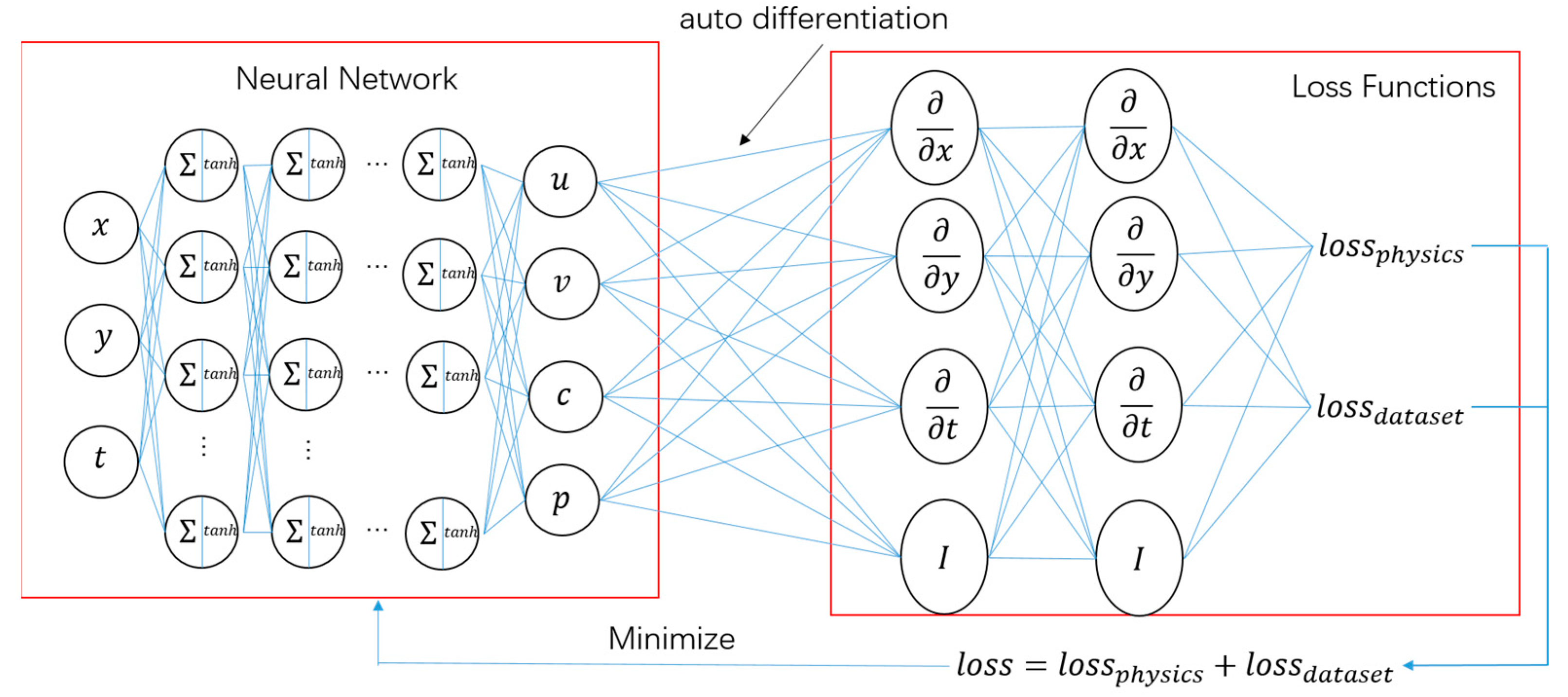
Figure 1. Architecture of the physics-informed neural network for fluid dynamics (note that the concentration field is the only observable).
Atmosphere 14 00759 g001
Figure 2. Schematic of bridge and geometric dimensions of bridge deck section: (a) Schematic of bridge; (b) bridge deck section.
Atmosphere 14 00759 g002
Figure 3. Geometric dimensions of fluid flow past a generic bridge deck section: (a) Geometric dimensions; (b) Mesh distribution.
Atmosphere 14 00759 g003
Figure 4. Training data for Re = 1250: (a) Concentration field for Re = 1250 at T = 46–50; (b) Concentration field for Re = 1250 at T = 46.
Atmosphere 14 00759 g004
Figure 5. Training data for Re = 5000: (a) Concentration field for Re = 5000 at T = 28.8–30; (b) Concentration field for Re = 5000 at T = 28.8.
Atmosphere 14 00759 g005
Figure 6. Comparison between predicted data and CFD data for Re = Pe = 1250: (a) u component; (b) v component; (c) p; (d) c; (e) mean absolute error.
Atmosphere 14 00759 g006
Figure 7. Comparison between predicted data and CFD data for Re = 5000: (a) u component; (b) v component; (c) p; (d) c; (e) mean absolute error.
Atmosphere 14 00759 g007
Figure 8. A micro-element taken on the surface of the geometry.
Atmosphere 14 00759 g008
Figure 9. The total stress on the micro-element, including two normal stresses as well as two identical tangential stresses.
Atmosphere 14 00759 g009
Figure 10. Lift and drag forces on micro-elements.
Atmosphere 14 00759 g010
Figure 11. Reference aero force and predicted aero force at Re = 1250: (a) drag coefficient; (b) lift coefficient.
Atmosphere 14 00759 g011
Figure 12. Reference aero force and predicted aero force at Re = 5000: (a) drag coefficient; (b) lift coefficient.
Atmosphere 14 00759 g012
Table 1. Parameters for different cases.
R e P e ν λ ρ T U B
125012501/12501/125015011
500050001/50001/500013011
Table 2. Hyperparameters in PINN model.
LnNnHBcLrBsIBs
1064TanhIbc0.00110,0002000
Table 3. Mean ϵ for u, v, and p separately and together.
  ϵ u ϵ v ϵ p ϵ
Re = Pe = 12500.01570.01230.03750.0218
Re = Pe = 50000.01960.01500.03940.0247
Table 4. The percentage form of error in Re = Pe = 1250.
Re = Pe = 1250MaxMin ϵ ϵ p e r
u1.3001−0.07850.01571.14%
v0.4747−0.41820.01231.38%
p0.5175−0.59920.03753.36%
Table 5. The percentage form of error in Re = Pe = 5000.
Re = Pe = 5000MaxMine ϵ p e r
u1.4644−0.33970.01961.09%
v0.6161−0.59940.01501.23%
p0.5512−0.87680.03942.76%
Disclaimer/Publisher’s Note: The statements, opinions and data contained in all publications are solely those of the individual author(s) and contributor(s) and not of MDPI and/or the editor(s). MDPI and/or the editor(s) disclaim responsibility for any injury to people or property resulting from any ideas, methods, instructions or products referred to in the content.