Abstract
The emission of black carbon (BC) particles, which cause atmospheric warming by affecting radiation budget in the atmosphere, is the result of an incomplete combustion process of organic materials. The recent wildfire event during the summer 2019–2020 in south-eastern Australia was unprecedented in scale. The wildfires lasted for nearly 3 months over large areas of the two most populated states of New South Wales and Victoria. This study on the emission and dispersion of BC emitted from the biomass burnings of the wildfires using the Weather Research Forecast–Chemistry (WRF–Chem) model aims to determine the extent of BC spatial dispersion and ground concentration distribution and the effect of BC on air quality and radiative transfer at the top of the atmosphere, the atmosphere and on the ground. The predicted aerosol concentration and AOD are compared with the observed data using the New South Wales Department of Planning and Environment (DPE) aethalometer and air quality network and remote sensing data. The BC concentration as predicted from the WRF–Chem model, is in general, less than the observed data as measured using the aethalometer monitoring network, but the spatial pattern corresponds well, and the correlation is relatively high. The total BC emission into the atmosphere during the event and the effect on radiation budget were also estimated. This study shows that the summer 2019–2020 wildfires affect not only the air quality and health impact on the east coast of Australia but also short-term weather in the region via aerosol interactions with radiation and clouds.
1. Introduction
Black carbon (BC) is produced from the incomplete combustion of organic materials and is strongly related to elemental carbon (EC). They absorb light at various wavelengths from visible to near-infrared spectra. Brown carbon (BrC) mostly consists of organic carbon (OC) aerosols emitted from combustion sources such as biomass burnings and fossil fuel combustion and absorbs light from near-ultraviolet to visible range. The total carbonaceous aerosol light absorption consists of BC and BrC contributions in which BC light absorption dominates the total absorption. Feng et al. 2013 [1], in their global simulation study on the radiative effect of total carbonaceous aerosols, showed that BrC absorption can introduce a warming effect up to 0.11 W·m−2 at the top of the atmosphere (TOA), which is about one-quarter of that by BC absorption at the TOA. Pani et al., 2021 [2], in their study of BrC over an urban site in Chiang Mai, northern Thailand, found that BrC light absorption during the biomass burnings in peninsular Southeast Asia at the end of the dry season in 2016 was significant in five measurement channels of the aethalometer.
Reducing BC emissions has co-beneficial effects, as this reduces its harmful effect on air quality and health and also mitigates warming climate change. As a component of PM2.5, BC has a harmful effect on the exposed population. Anenberg et al., 2011 [3] used the global chemical transport model, called the Model for Ozone and Related Chemical Tracers (MOZART-4), to simulate PM2.5 concentrations and to calculate premature cardiopulmonary and lung cancer deaths. They showed that halving global anthropogenic BC emissions will reduce the outdoor population-weighted average of PM2.5 by 0.542 μg m−3 (1.8%), hence avoiding 157,000 annual premature deaths globally.
Compared to sulphate aerosols that scatter light and have a cooling effect, a reduction in sulphate aerosols instead results in a warmer climate. To determine the changes in temperature and precipitation to each perturbation of climate-forcing agents such as methane (CH4), carbon dioxide (CO2), black carbon (BC), sulphate (SO4) and solar insolation, the Precipitation Driver Response Model Intercomparison Project (PDRMIP) was established to drive identical perturbation inputs of forcing agents to different models based on the standard PDRMIP protocol [4]. Stjern et al., 2017 [5] studied climate response to increased concentrations of BC as part of the PDRMIP. They reported a weak surface temperature response to increased BC concentrations compared to other forcing agents and an even tenfold increase in BC, simulated by nine global coupled climate models, only produced a model median effective radiative forcing of 0.82 (ranging from 0.41 to 2.91) W·m−2, and a warming of 0.67 (0.16 to 1.66) K globally. Takemura and Suzuki 2019 [6], using climate simulation, also showed that BC’s positive effect on surface temperature is only one-eighth that of sulphate aerosols, which have cooling effect on the climate. However, Lou et al. 2019 [7] used a simulation of the global model, the community Earth system model (CESM) with the four-mode modal aerosol module (MAM4) and the aging processes of primary carbonaceous aerosols, which showed that an increase in BC emissions can increase the frequency of El Niño–Southern Oscillation (ENSO) extreme events.
The BC impacts on climate are through aerosol–radiation and aerosol–cloud interactions and the BC snow–albedo effect on top of land and sea ice. In addition to the effect of aerosol interaction with radiation changing the energy budget (direct effect), aerosol–cloud interactions (indirect effect), and heating the air and changing the boundary layer height (semi-direct), the change in cloud formation from aerosols, in turn, change the pattern of incoming and outgoing radiation (indirect effect). The aerosol layers can affect cloud formation in various ways depending on they are over land or sea and on the vertical distribution of aerosols. Aerosols act as cloud condensation nuclei (CCN) and the addition of aerosol particles affects cloud formation. A small increase in CCN in deep convective clean clouds causes more droplets to reach supercooled levels, increasing the amount of latent heat release and invigorating convection. However, greater CCN levels, above a critical concentration of 0.4% supersaturation, causes direct radiative effects dominating, cooling the surface and inhibiting convection [8]. Forkel et al. 2012 [9], using WRF–Chem, studied the direct, semi-direct and indirect effect of aerosols over central Europe. They showed that the inclusion of an indirect effect due to cloud cover and water content changes affects not only the precipitation change but also the concentration of air pollutants such as PM10.
As for precipitation effect, using model for interdisciplinary research on climate (MIROC5.2), a global climate model, Zhao and Suzuki 2019 [10] showed that BC causes a decrease in global annual mean precipitation, consisting of a large negative tendency of a fast precipitation response while SO4 also causes a decrease in global annual mean precipitation, which is dominated by a slow precipitation response.
The summer 2019–2020 wildfires in south-eastern Australia were the most extensive wildfires in Australia in terms of duration and spatial coverage. The wildfires started in late October 2019 in northern New South Wales (NSW); then, further wildfires occurred in the Blue Mountains and along the NSW south coast to Victoria. The burned areas mostly covered the forest in the national parks of NSW and Victoria, remote bushlands and areas surrounding some urban areas. As BC is a global warming agent and affects the health of the exposed population, it is important to estimate the amount of BC emissions into the atmosphere and the fate of BC from emissions to transport and deposition from the summer wildfires 2019–2020 in south-eastern Australia. Emission estimates from wildfires and an atmospheric model, i.e., WRF–Chem, are used to achieve this aim by analysing the output and the wildfires’ effect on BC transport and air quality across NSW and radiation budget. In addition, the Department of Planning, Industry and Environment (DPIE) of NSW has a network of aethalometers measuring the equivalence BC (eBC), providing valuable data for analysis and comparison. A previous study [11] showed that ground level diurnal BC concentration is strongly influenced seasonally and its composition in PM2.5 varies depending on urban and nonurban area where biomass burning is more dominant than fossil fuel combustion sources. As the wildfires were widespread and intense on a monthly scale, it is also an ideal situation to study aerosol interaction with radiation and cloud, as their signals were strong enough to be modelled.
The impact of aerosols from biomass burnings on weather and climate have been examined in several studies [8,12,13]. The short-term effects of aerosols during the wildfires have been known to impact local meteorological conditions, especially clouds and precipitation. WRF–Chem was used in these studies to include aerosol feedback or aerosol interactions with radiation and clouds. Chen et al. 2012 [13] showed that using moderate resolution imaging spectroradiometer (MODIS) satellite aerosol optical depth (AOD) assimilation in WRF–Chem improved the prediction of PM2.5 and OC, and in the fire downwind region, scattering aerosols cooled layers both above and below the aerosol layer and suppressed convection and cloud formation. This led to an average of 2% precipitation decrease during the wildfires of 13–18 August 2012 in the U.S. Archer-Nicholls et al. 2016 [8], in particular, applied WRF–Chem to wildfires during the 2012 fire season in Brazil to study the direct, semi-direct and indirect effect of aerosols on radiation, clouds and meteorology. This study also studies aerosol feedback using WRF–Chem during the 2019–2020 summer wildfires in southeast Australia.
The aim of this study is to determine the effect of the Black Summer 2019/2020 wildfires in south-eastern coast of Australia in terms of emissions, dispersion and transport of black carbon, its impact on air quality and radiation effect in the atmosphere using simulation with the WRF–Chem model.
2. Data and Methods
The WRF–Chem atmospheric model has recently been used by various authors in simulation studies of aerosols including BC emissions from natural events such as dust storms and wildfires or anthropogenic emissions from biomass burnings and combustion sources [14,15,16,17,18]. With respect to the east coast of Australia, previous studies [19,20] used WRF–Chem to predict the effect of the February 2019 dust storm and the 2019–2020 wildfires in south-eastern Australia on air quality and health impact. The predicted PM2.5 concentration allowed the impact on health of the population to be estimated. In this study, the same WRF–Chem model is used, but the focus is on BC. BC is an important pollutant emitted from the combustion process not only because of its harmful effect on health but its effect on radiation budget due to its solar and infrared radiation absorption property and hence climate effect.
The BC emission data from the wildfires were obtained from the Fire Emission Inventory from the NCAR (FINN) database. The FINN database provides the estimated emission of many pollutants including BC for use in WRF–Chem on a daily basis with 1 h time resolution and approximately 1 km2 spatial resolution globally. The dataset is available for three different air chemistry mechanisms: GEOS-CHEM (Goddard Earth Observing System Atmospheric Chemistry), MOZART-4 (Model for Ozone and Related Chemical Tracers 4) and SAPRC99 (State-Wide Air Pollution Research Center, Version 1999). In this study, the FINN dataset for the MOZART chemical mechanism is used in WRF–Chem to study the dispersion and concentration of BC during the 2019–2020 Black Summer wildfires. Figure 1 summarises the total aggregated of hourly estimated emissions of BC across the southeast Australia domain (Figure 2b) during the period from 1 November 2019 to 7 January 2020 of wildfires. This pattern of BC emission across the domain is comparable to that of PM2.5 concentration and health effect (such as mortality) as shown by Nguyen et al. 2021 [20] during this period. Overall, the total BC emission during the wildfire period from 1 November 2019 to 7 January 2020 in southeast Australia is approximately 92,000 tons of BC.
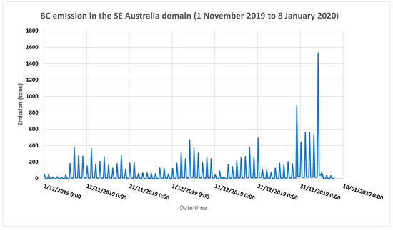
Figure 1.
BC hourly emissions as estimated from FINN during the period from 1 November 2019 to 7 January 2020 of wildfires in southeast Australia. Date and time are in GMT.
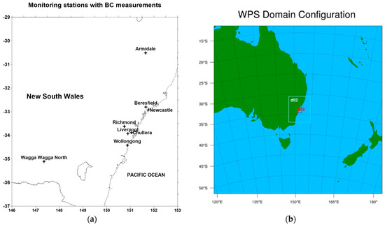
Figure 2.
(a) Aethalometer network in NSW operated by DPIE. (b) WRF–Chem domain configuration with domain d02 covering most of eastern NSW and domain d03 covering the greater metropolitan region (GMR) of Sydney.
The BC concentration prediction from WRF–Chem is evaluated against the observed equivalent BC (eBC) as measured using the aethalometer network of the DPIE of New South Wales (NSW) as shown in Figure 2. The aethalometers at the monitoring stations are the seven-channel aethalometer model AE33 from Magee Scientific. The details of this aethalometer network of stations and measurements was provided in a previous study [11]. The method of measurement of absorption or attenuation of light at different wavelengths to obtain equivalent BC (eBC) from wood burning and fossil fuel in AE33 is based on the work of Sandradewi et al. 2008 [21]. The AE33 aethalometer model uses the absorption Ångström exponent (AAE) in the λ−α spectral dependency as α = 1 for fossil fuel and α = 2 for wood burning. These AAE values for the sources are also dependent on emission characteristics at the location and seasonal period when measurements are made. Tobler et al. 2021 [22] calibrated the AE33 aethalometer using measurements made in Krakow, Poland to select the suitable values of α = 0.89 for traffic (fossil fuel combustion) and α = 1.9 for solid fuel sources (wood burning and coal burning). In NSW, domestic coal burning is mostly non-existent, while the remaining 2 coal-fired power stations are being phased out. In our study, the standard AE33 aethalometer model is used with AAE as 1 for traffic (fossil fuel) and 2 for wood burning (or biomass burning). The AAE can be calculated from the light absorption coefficients at different wavelengths used in the AE33 aethalometer. These real-time values of AAE reflect the BC composition in the air measured at the time. The time series of AAE hourly values during the wildfire period from 1 November to 31 December 2019 are summarized in the histogram for each of the aethalometer monitoring sites and are shown in Appendix A.
The reanalysis products from NASA Modern-Era Retrospective Analysis for Research and Applications, Version 2 (MERRA-2) and observed aerosol optical depth (AOD) from remote sensing MODIS Terra/Aqua satellites are used to compare and validate the modelled aerosols, including BC, as predicted using WRF–Chem. The 3 km aerosol products MYD04-3k (Aqua) and MOD04-3k (Terra) provide AOD over ocean and land. In addition, AOD from AERONET ground lidar stations at Lidcombe station, located in Sydney, is used to compare with the predicted AOD.
The modelling domain covers the eastern half of Australia including the southeast coastal areas where the wildfires occurred and is based on Lambert projection with 386 × 386 grid points at resolution 12 km × 12 km as shown in Figure 2b. There are 32 model vertical sigma levels with the centre of the domain coordinate at 150.994° longitude and −33.921° latitude.
The configuration of WRF–Chem V4.2 in this study used the following science options: land surface based on the Noah land surface model (a unified NCEP/NCAR/AFWA scheme with soil temperature and moisture in four layers), the Monin–Obukhov similarity method for surface layer physics, the Yonsei University (YSU) scheme for planetary boundary layer (PBL), microphysics based on double-moment Morrison parameterisation (mp_physics = 10) for modelling indirect effect on radiation due to aerosol cloud interaction, the rapid radiative transfer model (RRTMG) with aerosol feedback for shortwave and longwave radiation, gaseous MOZART-4 chemistry and the model for simulating aerosol interactions and chemistry (MOSAIC) aerosol model (chem_opt = 202), Maxwell–Garnet method for aerosol extinction coefficient approximation, the Goddard Chemistry Aerosol Radiation and Transport–Air Force Weather Agency (GOCART–AFWA) dust emission scheme, and the Kain–Fritsch scheme for the cumulus cloud model. In addition, wet scavenging and cloud chemistry options are turned on (wetscav_onoff = 1; cldchem_onoff = 1) and the prognostic number density option is set (progn = 1) so that particle microphysics with double moment can be activated. A summary of the science options used in WRF–Chem for this study is provided in Table 1.

Table 1.
WRF–Chem configuration with science options in this study.
Anthropogenic emission is obtained from the global 2005 anthropogenic Emission Database for Global Atmospheric Research (EDGAR) version 4 compiled for the Task Force on Hemispheric Transport of Air Pollution (TF-HTAP). Inline MEGAN biogenic emissions and sea salt emissions were chosen in this study. In a previous study, the MOZART gaseous chemistry and aerosols GOCART chemistry (MOZCART) was used. In this study, MOZART/MOSAIC is used as the aerosol MOSAIC module accounts for optical properties of different aerosols and its aqueous chemistry treatment can better represent the interactions among aerosols, chemistry and clouds for determining aerosol indirect effect on radiation. The MOSAIC aerosol module in WRF–Chem also computes quickly and efficiently [23].
As BC has hygroscopic properties or the ability to absorb moisture from air, in WRF–Chem simulation using MOZCART chemical mechanism, there are two types of BC: hydrophobic and hydrophilic BC. The BC aging process from fresh hydrophobic BC emissions to hydrophilic BC involves water uptake. BC from fresh emissions from biomass combustion is hydrophobic BC, which then undergoes accumulation of gases, water vapour and particle formation process and mainly becomes hydrophilic BC. The model predicts both hydrophobic and hydrophilic BC. In MOZART-4 and MOZCART models, the BC input emission into the models is initially split into 80% hydrophobic BC (BC1) and 20% hydrophilic BC (BC2). It is assumed that freshly emitted BC1 is transformed into BC2 with a fixed ageing rate of 2.5 days. BC2 is then considered as an aged pollutant transported from non-local emission sources [15]. BC modelling is based on MOZART-4/GOCART option in WRF–Chem.
In a study on long-range transport of BC to the Pacific Ocean from different global emission sources and its dependence on aging timescale, Zhang et al. 2015 [24] used the lifetime, which is related to aging timescale, of BC emitted from Australia as 5.3 days, optimised with observed data, which is higher than the average of all sources.
There are two methods of calculating direct radiative forcing (DRF) by aerosols, one is running a control model run without aerosols (no emission input) and one with aerosols. This was used in Chaibou et al. 2020 [14] for dust DRF in dust storms over Africa. The other method is using a diagnostic procedure in WRF–Chem as performed in several studies [17,18,25]. The diagnostic procedure is simpler and less time consuming. This method, first proposed by Zhao et al. 2013 [17], for calculating the DRF (and AOD) for each aerosol type, involves the calculation of aerosol radiative transfer and optical properties to be performed multiple times with the mass of one aerosol species and its associated water aerosol mass removed from the calculation each time. Then, after this diagnostic iteration procedure, the DRF for an individual aerosol species is estimated by subtracting the DRF from the diagnostic iterations from those estimated following the standard procedure for all the aerosol species (Appendix C).
In this study, the first method is adopted, as it is simpler. To determine the BC aerosol’s direct, semi-direct and indirect effects on radiation, the following two WRF–Chem runs were performed: BASE scenario, with all emissions and aerosol-radiative interactions on and the NOEMISS scenario, with the emission source of interest removed. Another method that can be used to achieve the same end is to make two runs. Run 1 is the same as “BASE” above while, in Run 2, the absorption profile of BC is modified to exclude it in the RF calculation. In WRF–Chem, the code is changed with ref_index_bc = cmplx (1.85, 0.71) being replaced by ref_index_bc = cmplx (0, 0).
To determine the direct SW radiative forcing (SWDIRECT), defined as the difference in upwelling SW radiation between the FE (fire emission) and nFE (no fire emission) scenarios (the downwelling is the same in both scenarios), we follow the equations used in a previous study [26]
after adjusting for the radiative effects of water vapour to be removed by subtracting the clean-sky value (the second term on the right-hand side of the above equation). The aerosol radiation forcing (RF), as specified in Equation (1) above, describes the perturbation in flux in the atmosphere caused by the presence of the aerosol layers in relation to that calculated under clear-sky conditions [27]. SWDIRECT Radiation Forcing (RF) is sometimes denoted as RFSW, DIRECT. The net RF is the sum of short-wave RF and long-wave RF
SWNET = SWDIRECT + LWDIRECT
Similarly, the indirect effect is calculated with no aerosol radiative interactions (nARI) as
This requires another run with fire emission on, but the aerosol radiative feedback is off (aer_ra_feedback = 0 in WRF_Chem namelist.input)
The semi-direct effect is obtained after subtracting the direct and indirect effects from the change in upwelling SW radiation at the TOA:
To validate the meteorology component of the model, in addition to surface meteorological observed data such as wind speed, wind direction and temperature, ideally, we can also use the observed mixing level height as measured by radiosonde data from a number of sites. As the WRF–Chem simulation in this study used the YSU PBL scheme, the bulk Richardson number method was used to calculate the PBL height (PBLH). DPIE also has the Vaisala lidar ceilometers CL51 providing PBLH. As the ceilometers were installed after the Black Summer Wildfires of 2019–2020, the PBLH prediction cannot be validated. However, in our previous study [28], the predicted PBLH was compared with CL51 boundary layer height measurement and the YSU PBL scheme in the current WRF–Chem setup model provided good results.
3. Results and Discussion
3.1. Ground Concentration and Spatial Pattern of BC during the Wildfires
BC measurements from AE33 aethalometers at DPIE monitoring sites from 1 November to 15 January 2020 showed a high concentration of BC due to biomass burning or wood burning (BCwb) as compared with BCff concentration. According to the aethalometer model used in AE33, BC concentration measurements consist of BC from wood burning and BC from fossil fuel combustion and these BC components can be derived using different light absorption characteristics of BC from wood burning and fossil fuel combustion at the 470 nm wavelength (near-UV) channel and 950 nm wavelength (near IR) channel. By analysing different channels of aethalometer measurements, the BCff (from fossil fuel) and BCwb (from wood burning or biomass burnings) or BCbb (percentage of biomass burnings) can be estimated.
Figure 3 shows the concentration of BC components BCwb and BCff during the wildfires period at all aethalometer measuring sites: Liverpool, Chullora, Wagga Wagga North, Armidale, Wollongong and Richmond during December 2019.
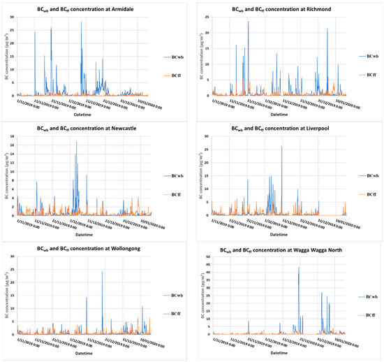
Figure 3.
Observed BCwb and BCff hourly concentration at Armidale, Richmond, Newcastle, Liverpool, Wollongong and Wagga Wagga North during the wildfire period 1 November 2019 to 15 January 2020.
The time series of BC concentration at various sites reflects the progress of the Black Summer 2019–2020 wildfires in southeast Australia during this period. Fires started in early November 2019 in northern NSW and the Gospers Mountain in the Blue Mountains, northwest of Sydney, which then spread to most of the Blue Mountains, west of Sydney, and lasted for most of December 2019. Then, fires occurred in the Southern Highland, the South Coast, south of Sydney, to the border region of Victoria in late November 2019 until 7 January 2020 when fires subsided. From 8 January 2020, no more wildfires occurred in NSW but still occurred in northeast Victoria until the middle of January. Remote sensing data of hot spots from MODIS Terra/Aqua satellites as shown in Figure 4 show the progress and extent of the wildfires. Wildfires began in northern NSW and the Blue Mountains in early November 2019 (Figure 4a). BCwb concentrations were high in November at Armidale in northern NSW, Richmond and Liverpool in the northwest and west of Sydney, especially on 21 November 2019, when smoke covered most of northern NSW and smoke from fires in the Gospers Mountain of the Blue Mountains drifted to the west of Sydney (Figure 4b). By early December 2019, wildfires started occurring at the NWS and Victoria border near the coast (Figure 4c). High concentrations of BCwb were detected on 11 December 2019 at Newcastle, Liverpool and Wollongong when fires in the Blue Mountains, Southern Highlands were intense. On this day, fires in the South Coast also affected Canberra (Australian Capital Territory), as shown in Figure 4d. High concentrations of BCwb also occurred in Wollongong, Wagga Wagga and Richmond, Liverpool in Sydney on 21 and 30 December 2019 when fires in the Blue Mountains, Southern Highland and South Coast covered most of NSW with smoke (Figure 4e,f).
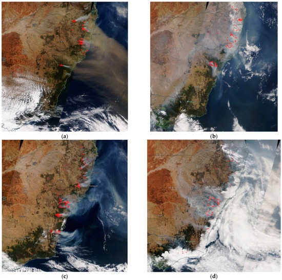
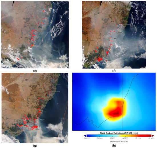
Figure 4.
MODIS Terra/Aqua satellite image and hot spots over southeast Australia on 7 November 2019 (a), 21 November 2019 (b), 5 December 2019 (c), 11 December 2019 (d), 21 December 2019 (e), 30 December 2019 (f), and 4 January 2020 (g). Average BC extinction AOT at 550 nm for March 2020 as predicted by MERRA-2 (h) (Source: NASA Worldview and NASA https://giovanni.gsfc.nasa.gov/, accessed on 11 April 2022).
Simulation of BC emissions from wildfires and dispersion of emitted pollutants using the WRF–Chem model was performed for the period from 1 November 2019 to 8 January 2020. As in a previous study [20], the prediction of surface meteorological variables was compared with observation at the monitoring stations and the meteorological performance is shown in Figure A2 of the Appendix B. The simulation allows us to understand the spatial pattern of BC concentration due to wildfires across NSW. The predicted total ground concentration of BC was compared with BC, as measured using an aethalometer at the sites in the DPIE network. Figure 5 shows the predicted daily BC concentration as compared with observations at Armidale, Richmond, Newcastle, Liverpool, Wollongong and Wagga Wagga North. The predicted BC is underestimated at most of the sites as compared with observations, but most of the patterns of daily BC change are similar. This is due either to the emission from FINN, or the meteorological prediction’s inaccuracy. As the meteorological variables such as the wind have been shown to be performed well, it is more likely that the emission from FINN was underestimated.
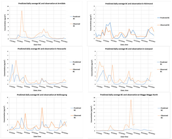
Figure 5.
Predicted daily total BC and observed BC in micrograms/m3, as measured using aethalometers at Armidale, Richmond, Newcastle, Liverpool, Wollongong and Wagga Wagga North during December 2019 period. Correlation coefficients of predicted and observed data at these sites are 0.41, 0.61, 0.58, 0.60, 0.24, 0.78, respectively.
Underprediction of BC concentration was also reported in a WRF–Chem simulation based on CB05 and aerosol modules in previous research [29]. In their study of sensitivity of simulated chemical concentration and aerosol–meteorology interactions to aerosol treatments and biogenic organic emissions, they used WRF–Chem with CB05 (Carbon Bond v.5) for gas-phase chemistry and three different aerosol modules: the modal aerosol dynamics model for Europe/secondary organic aerosol model (MADE/SORGAM), the model for simulating aerosol interactions and chemistry (MOSAIC), and the model of aerosol dynamics, reaction, ionization and dissolution (MADRID) to simulate aerosols over continental U.S. for January and July 2001 from anthropogenic and biogenic emission sources. For BC prediction, they reported all simulations showing large underpredictions in BC at the SEARCH sites; moderate underpredictions only occurred at the IMPROVE sites from the simulation with MADE/SORGAM. Such underpredictions were attributed mainly to the underestimation in BC emissions. They suggested the difference in WRF–Chem performance using different aerosol modules was likely due to different PBL meteorology from different gas and aerosol predictions providing different feedbacks to meteorology and different dry deposition fluxes resulting from different aerosol size representations and methods for solving coagulation and gas/particle partitioning processes that affect the growth of aerosols between MADE/SORGAM and the two other aerosol modules.
However, as compared to the MERRA-2 BC prediction, the WRF–Chem BC prediction is closer to observation. Figure 6 shows the predicted time series of MERRA-2 and WRF–Chem as compared to that of the observation at the monitoring sites.
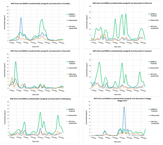
Figure 6.
WRF–Chem and MERRA-2 prediction of daily average BC concentration for December 2019 as compared to BC measured at monitoring sites (Armidale, Richmond, Newcastle, Liverpool, Wollongong and Wagga Wagga North).
Spatial distribution of BC surface concentration as predicted using WRF–Chem can also be compared with MERRA-2 reanalysis hourly 2D model prediction (MERRA-2 tavg1_2d_aer_Nx, Single-Level, Assimilation, Aerosol Diagnostics) at 0.5° (lat) and 0.625° (lon). Figure 7 shows the BC concentration contour as predicted from MERRA-2 and WRF–Chem on 5 December 2019 13:00 local time or AEST (Australian Eastern Standard Time) and 21 December 2019 13:00 AEST. The spatial patterns are similar but, the magnitude of the predicted concentrations of BC are mostly smaller than those of MERRA-2. WRF–Chem predictions at various sites are closer to observation as compared to the MERRA-2 prediction.
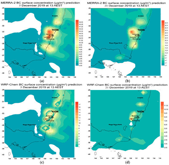
Figure 7.
MERRA-2 reanalysis model prediction of surface BC on 5 December 2019 13 AEST (a) and on 21 December 2019 13 AEST (b). WRF–Chem prediction of BC on 5 December 2019 13 AEST (c) and 21 December 2019 13 AEST (d).
The WRF–Chem BC prediction is lower as compared to predictions from MERRA-2, as shown in Figure 6. This is expected, as MERRA-2’s output is at coarse resolution at 0.5° by 0.625° (lat–lon, ~50 km and ~60 km) while WRF–Chem is at 12 km by 12 km resolution. MERRA-2 is a reanalysis modelling system that considered and assimilated observed data from ground and remote sensing data from satellites. At some of the monitoring sites, the predicted time series of BC as derived from the grid point in MERRA-2 and WRF–Chem provides different results. The MERRA-2 grid cells encompassing the fire sources provided high concentrations as compared to those based on the grid cells in WRF–Chẹm.
Zhao et al. 2014 [18] conducted a simulation and measurement study of BC, dust and their radiative forcing over North China using WRF–Chem, as in our study. They found that the simulated spatial variability of BC and dust mass concentrations in the top snow layer are consistent with observations. However, the model, in general, moderately underestimated BC on the snow layer in the clean regions but significantly overestimated BC in some polluted regions. As Curci et al. 2015 [30] showed in their study of chemical and dynamical processes leading to the formation of aerosol layers in the upper planetary boundary layer (PBL) and above it, the vertical mixing and entrainment into the PBL from these layers can contribute to the ground-level particulate levels. The 2019–2020 wildfires produced significant layers of aerosols in the atmosphere including the layers above the PBL. The WRF–Chem model simulated the chemical and dynamical processes within the PBL but the dynamic interaction process between upper level above PBL in the stratosphere and the top of PBL is not captured. Figure 8 shows the difference in BC surface mass concentration and column mass density, which takes into account BC layers above ground and above PBL.
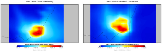
Figure 8.
Spatial pattern of monthly average BC column mass density and BC surface mass concentration in March 2020 as predicted by MERRA-2.
3.2. Vertical Distribution and Transport of BC
The dispersion of the BC plume from the summer 2019–2020 wildfires into the atmosphere and its advective transport was extensive across the Tasman Sea to New Zealand and at time to South America as reported in a previous study [20]. Figure 9 shows the BC plume at 850 mb (~1450 m) reached the North Island of New Zealand on 5 December 2019 from wildfires in northern NSW, the Blue Mountains and the South Coast of NSW. BC aerosol plumes at 700 mb (~3000 m) above sea level were predicted above the Tasman Sea off the coast of NSW.
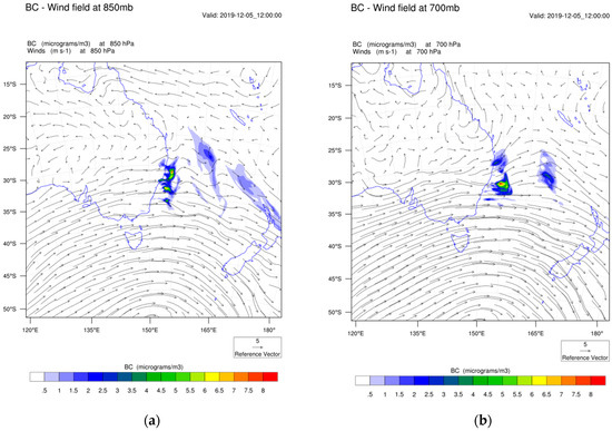
Figure 9.
BC concentration and wind field at 850mb (~1450 m) (a) and 700 mb (~3000 m) (b) on 5 December 2019 12:00 UTC (5 December 2019 22:00 AEST).
Singh et al. 2020 [15] used WRF–Chem and FINN biomass emission data to study the BC transport from the lower PBLH to higher altitudes in the troposphere above South Asia during active convection periods in 2013. They reported that the free troposphere BC concentration is higher in the monsoon season compared to in the winter season at the same elevation and the presence of a persistent BC plume from 500 hPa. The transport of air pollutants in the upper air depends on accurate modelling of the PBL. There are other schemes in the WRF model for calculating the PBLH such as one based on turbulent kinetic energy or the use of observed profile data from radiosonde to estimate the PBLH as discussed by Shi et al. 2020 [31].
With denser monitoring data from the deployment of some low-cost PM2.5, such as used in Armidale, NSW [32], large spatial variation in PM2.5 can be captured, better modelling and estimation of health impact can be achieved. As the aethalometer network is very sparse, modelling of BC emissions and dispersion to predict the BC concentration is required to provide high resolution spatial BC distribution. Future instalment of micro-aethalometer BC sensors can improve the observed coverage and provide better validation of the model, especially in the western NSW region.
For a future modelling study of BC, we will also use the recent data from the two new ceilometers installed in the Sydney region and in the northwest of Sydney to better understand the evolution of PBLH and its relationship with ground BC concentration as well as to validate the PBLH estimate in the WRF–Chem model [28].
3.3. Radiative Forcing
Singh et al. 2020 [16] used WRF–Chem to simulate the dispersion and transport of carbonaceous carbon (BC and OC) from biomass burning in South Asia with emission data from FINN for 2013. They reported radiative forcing of up to −6.14 W·m−2 and −0.50 W·m−2, −42.76 W·m−2 and −1.91 W·m−2 at the surface and at the top of the atmosphere over Punjab and Myanmar, respectively, and that the surface temperature decreased by 2 K.
Lin et al. 2014 [25], in their study of aerosol transport to Taiwan from biomass burnings in Southeast Asia using WRF–Chem during the period 15–18 March 2008 reported that 34% of the AOD was attributed to OC over Indochina, while the contribution of BC to AOD was about 4%. Biomass-burning aerosols over Indochina also had a net negative effect (−26.85 W·m−2) at ground surface, a positive effect (22.11 W·m−2) in the atmosphere and a negative forcing (−4.74 W·m−2) at the top of atmosphere (TOA). Aerosol plumes stretching from southern China to Taiwan caused a reduction in shortwave radiation of about 20 W·m−2 at ground surface.
Papanikolaou et al. 2022 [27], in their study of the optical properties and radiation forcing of the particles in the troposphere and stratosphere originated from the Australian wildfires 2019/2020 using CALIPSO satellite data, found that aerosol smoke particles in the stratosphere are mainly fine and ultrafine particles while coarser particles in the troposphere over the region bounded between the longitude range from 140° E to 20° W and latitude range from 20° to 60° S (from the east coast of Australia to South America). In terms of radiative forcing, they found that the tropospheric smoke layers had a negative mean radiative effect, ranging from −12.83 W/m2 at the TOA, to −32.22 W/m2 on the surface (SRF), while the radiative effect of the stratospheric smoke was estimated between −7.36 at the TOA and −18.51 W/m2 at the SRF.
In addition to aerosols, clouds and water vapour have an important role in the reflection and absorption of incoming solar radiation. Their effect is determined in the study of aerosol effect by using clear sky simulation to exclude their effects, then comparing the results with those when full clouds and water vapor are included. An example of cloud reflection and hence reducing net radiation from the results of simulation of the December 2019–2020 wildfires study is shown in Figure 10 for the simulated day of 1 December 2019 with MODIS observed and hot spots from fires. This day was cloudy with a cumulus cloud band from northern Australia and northern NSW to New Zealand. The simulation of shortwave (SW) downward and upwelling radiation at the TOA essentially captured the cloud reflection.
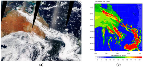
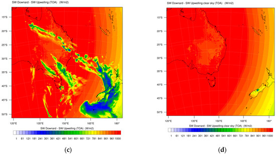
Figure 10.
MODIS observation on 1 December 2019 with red spots as fires (a) upwelling SW radiation at the TOA, (b) downward SW minus upwelling SW at TOA (c), and downward SW minus upwelling SW at TOA in clear sky situation (d), as simulated without fires on 1 December 2019 at 04 UTC.
Figure A3 in Appendix B shows the WRF–Chem simulation results of radiation at TOA on 1 December 2019 with wildfires taken into account. To visualise the difference in TOA SW radiation budget between wildfires and without wildfires and the effect of water vapour on downward and upwelling radiation, the SW differences at TOA simulated without and with wildfires and under vapour and without vapour scenarios are shown in Figure 11 for upwelling radiation. The water vapour can scatter and absorb radiation and its presence in the atmosphere do not change the radiation pattern much, with the net effect as noise over the main reflection and absorption pattern due to clouds and aerosols.
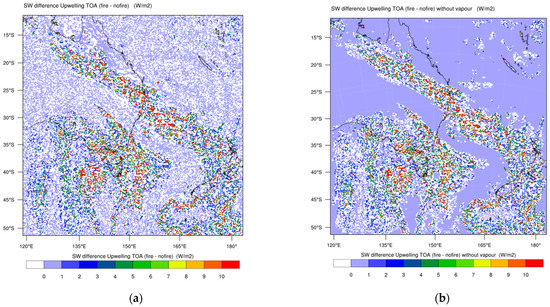
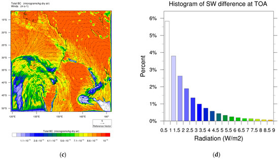
Figure 11.
Predicted difference in upwelling SW radiation between fire and no fire simulation with vapour (a) and without vapour (b) and predicted surface BC concentration with surface wind field (c) on 1 December 2019 04 UTC. Off the coast of NSW and eastern Australia, there were high BC concentrations from wildfires. The histogram of negative forcing values at TOA over the domain (d).
Figure 11 shows the difference in SW upwelling at TOA between wildfire and no wildfire simulation on 1 December 2019 and the surface BC concentration. It can be seen that the areas where low predicted concentration of BC also mostly corresponded with those covered by clouds and high concentration occurred where there were no clouds. The strong upwelling radiation was due to reflecting radiation from clouds and the low upwelling due to absorption of downwelling radiation occurred in areas with a higher concentration of BC.
The difference In SW radiation at the top of atmosphere (TOA) due to wildfires on 1 December 2019 is approximately −1.46 W/m2 on average over the modelling domain. The negative forcing at the TOA is mostly due to radiation cloud reflection. After adjusting for the radiative effects of water vapour (cloud) to be removed (−0.04 W/m2), the SW direct effect is about −1.42 W/m2 as specified in Equation (1). Figure 11d shows the distribution of TOA negative forcing values over the domain. At the surface, SW negative forcing due to wildfires on this day also occurred and is approximately −1.45 W/m2 (after removing the cloud effect) while the figure for LW is −0.55 W/m2. Hence, the net radiation forcing as provided in Equation (2) is RFNET = −2.0 W/m2. Figure A4 in Appendix B shows the predicted difference in upwelling SW radiation at the surface between the fire and no fire simulation. The simulated surface temperature at 2 m above ground (T2) as well as the PBL height on average over the domain is lower in the wildfire case than those in the no wildfire simulation.
The results can be compared with the Global Land Data Assimilation System (GLDAS) Catchment Land Surface (CLS) Model L4 V2.2 daily data at 0.25 × 0.25 degrees resolution as shown in Figure 12.
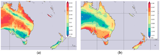
Figure 12.
Net short-wave (a) and long-wave radiation flux (b) on 1 December 2019 daily 0.25 deg. (GLDAS Model GLDAS_CLSM025_DA1_D v2.2). Unit measurement is in W/m2.
Archers-Nicholls et al. 2016 [8], in their study of biomass burnings in Brazil during September 2012 using WRF–Chem with nested domains at 5 km and 1 km horizontal resolution, reported that direct interactions between aerosols from biomass burning and radiation resulted in a net cooling effect. The average shortwave direct effect is −4.08 ± 1.53 W/m2. However, about 21.7 W/m2 is absorbed by aerosols in the atmospheric column, warming the atmosphere at the aerosol layer height, stabilising the column, inhibiting convection, and reducing cloud cover and precipitation. The semi-direct effects, from changes to clouds due to radiatively absorbing aerosols, increase the net short-wave radiation reaching the surface by reducing cloud cover, producing a secondary warming effect that counters the direct cooling. The shortwave semi-direct effect was sensitive to model resolution and convective parameterisation varying from 6.06 ± 1.46 W/m−2 with convective parameterisation to 3.61 ± 0.86 W/m−2 without convective parameterisation. The aerosols acted as CCN, increasing the droplet number concentration of clouds but had negligible impact on the net radiative balance. They also reported that the sensitivity to the uncertainties relating to the semi-direct effect was greater than any other observable indirect effects.
Curci et al. 2015 [30] noted that the assessment of the direct, semi-direct and direct effects of atmospheric aerosols is still characterized by large uncertainties. The confidence interval terms of radiation effects in the studies mentioned above are still large. Fierce et al. 2020 [33] showed that large discrepancies between observed and predicted radiation absorbed by BC in many studies are the results of two factors: first, the assumption of a spherical BC core shell generally led to the overestimation of BC absorption; and secondly, lower-than-expected absorption resulted largely from increases in particle-to-particle heterogeneity in which various BC particles accumulated or coalesced with others differently while the assumption of homogeneous particle within each mass class in the model caused higher absorption.
In addition to the physics and microphysics options, their uncertainties and feedback in the meteorological and air quality model, there are a number of other uncertainties regarding BC modelling using the MOZART/MOSAIC (or GOCART) chemistry option in WRF–Chem. One of the uncertainties is that the BC aging process is not fully captured. This process is a complex one in which the morphology, hygroscopicity and optical properties of BC are changed by coating it with other materials. BC aging leads to an increase in water uptake, change in morphology from fractal aggregate to sphere and increase in both absorption and scattering in the shortwave radiation [34,35]. The aging timescale is critical in the study of the long-range transport of BC, and its uncertainty was evaluated with observation in some studies such as Zhang et al. (2015) [24]. Wang et al. 2018 [35] suggested some constraints on the aging timescale, used in the community atmospheric model (CAM), based on environmental chamber measurements.
Another uncertainty is the estimation of BC emissions from the FINN database, which relies on satellite measurements of hotspots, and their radiative power with various types of vegetation during the wildfires. Underestimation of BC emissions as compared with other wildfire emission datasets such as GFED has been reported by Desservettaz et al. 2022 [36].
4. Conclusions
This study has used the WRF–Chem air quality model to study the emission and transport of BC during the Black Summer 2019–2020 wildfires in south-eastern Australia based on the fire emission inventory data from NCAR (FINN) and NCEP global meteorological data. The model, using the MOZART/MOSAIC chemical mechanism, can capture the spatial and temporal pattern of BC ground concentration corresponding closely with BC measurements from the aethalometer network in NSW and satellite and global MERRA-2 model data. The prediction of daily BC concentration from WRF–Chem is closer to the observation as compared to the MERRA-2-assimilated global product. This is mainly due to the higher spatial resolution used in WRF–Chem. MERRA-2 overpredicted while WRF–Chem underpredicted the BC concentration. The results of this study and other studies suggest that the emission from FINN is underestimated.
The 2019–2020 wildfires provided an ideal situation for studying BC emissions, transport and concentration at ground- and higher levels in the atmosphere. At the ground level, the predicted daily concentration of BC during the wildfire periods corresponds with the observation measurements from the DPE aethalometer monitoring network, and considering the uncertainties in the emission, meteorology and model in numerical modelling, the WRF–Chem model performed reasonably well in this respect. At higher altitude, above 1500 m, the BC pollutants as emitted from the wildfires were transported across the Taman Sea and reached New Zealand, as predicted from the model. This widespread transport of BC and aerosol clouds shows the extent of the effect of the 2019–2020 wildfires.
The WRF–Chem model also provides information on the radiation effect of aerosols including BC and other pollutants during the wildfire period. The BC and aerosol interaction with radiation and clouds via the direct, semidirect and indirect effect, as implemented in WRF–Chem, showed negative forcing at TOA and allowed for an understanding of the short-term effect of wildfire emissions of BC and aerosols on climate.
There are some limitations in this study, such as the underestimation of the BC emission from FINN and the uncertainties in the meteorological NCEP input data as well as the WRF–Chem model itself. Our future work will be focused on the improvement of emission data from wildfires by comparing different global emission datasets such as FINN and GFED and their refinements to provide better ground level prediction of BC using WRF–Chem.
Supplementary Materials
The following supporting information can be downloaded at: https://www.mdpi.com/article/10.3390/atmos14040699/s1, Excel of model data files to produce Figure 5, Figure 6 and Figure A2.
Author Contributions
Conceptualization, H.N.D., M.A., Y.Z. and M.R.; methodology, H.N.D., Y.Z., D.S. and S.W.; data procurement, J.K., D.S., T.T., J.C., G.G. and J.H.; formal analysis, H.N.D., Y.Z. and D.S.; investigation, H.N.D., Y.Z. and S.W.; writing—original draft preparation, H.N.D., L.T.-C.C. and K.M.; visualization, T.T. and H.N.D.; supervision, H.N.D., M.A. and M.R.; and project administration, H.N.D., M.A. and M.R. All authors have read and agreed to the published version of the manuscript.
Funding
Y.Z.’s time in this collaboration was supported by the U.S. NOAA Office of Climate AC4 Program (NA20OAR4310293).
Institutional Review Board Statement
Not applicable.
Informed Consent Statement
Not applicable.
Data Availability Statement
Data available upon request to the corresponding author. Analysis data are provided in the Supplementary Materials. WRF–Chem output NetCDF data is available upon request to the corresponding author.
Acknowledgments
The following data sources are gratefully acknowledged: the CALIPSO satellite products from the NASA Langley Research Center (Calipso Lidar Browse Images. Available online: http://www-calipso.larc.nasa.gov/products/lidar/browse_images/production//, accessed on 27 March 2021), the FINN fire emission datasets from the NCAR, U.S. (available online: http://www.acom.ucar.edu/acresp/MODELING/finn_emis_txt/; accessed on 27 March 2021), MODIS Aqua/Terra satellite hot spots data from the NASA, U.S., final analysis (FNL) reanalysis data from the National Center for Environmental Prediction (NCEP), U.S. The MERRA-2 data used in this study/project were provided by the Global Modeling and Assimilation Office (GMAO) at NASA Goddard Space Flight Center. Analyses and visualisations, where they are indicated in the paper, were produced with the Giovanni online data system, developed and maintained by the NASA GES DISC. Y.Z. acknowledged the support by the University of Wollongong (UOW) Vice Chancellors Visiting International Scholar Award (VISA), the University Global Partnership Network (UGPN) at North Carolina State University, U.S.A. and Australia’s National Environmental Science Program through the Clean Air and Urban Landscapes hub at University of Wollongong, Australia, that facilitated this collaboration.
Conflicts of Interest
The authors declare no conflict of interest.
Appendix A
The absorption Ångström exponent (AAE) of wavelength-dependent light attenuation is calculated at each aethalometer monitoring site for each hour during the wildfire period using the two wavelengths (470 nm and 950 nm) method.
First the light absorption coefficient at wavelength 470 nm is obtained as
where eBC is the equivalent BC as measured by the aethalometer and MAC is the mass absorption cross-section (MAC) at wavelength 470 nm. The MAC at 470 nm wavelength is factory set at the value of 14.54 as specified in the AE33 manual.
babs (470 nm) = eBC (470 nm) × MAC (470 nm)
Similarly, for wavelength 950 nm:
with MAC at 950 nm set as 7.19.
babs (950 nm) = eBC (950 nm) × MAC (950 nm)
The AAE of light attenuation is then determined as follows:
AAE = −ln((babs (470)/babs (950))/ln(470/950)
Figure A1 shows the histograms of AAE hourly values at four urban sites (Richmond, Liverpool, Wollongong, Newcastle) and two regional sites (Wagga Wagga and Armidale). At Armidale, the BC composition is mostly from biomass burning while other urban sites show some influence of fossil fuel combustion in the BC contribution.


Figure A1.
Histograms of hourly AAE for the period of 1 November to 31 December 2019 at Richmond, Liverpool, Wollongong, Newcastle (urban sites), Wagga Wagga and Armidale (regional sites).
Appendix B
Appendix B.1. Surface Meteorological Prediction and Observation at Bringelly and Newcastle
Correlation coefficients and index of agreement (IOA) for temperature and wind speed are 0.81 (r), 0.73 (IOA) and 0.68 (r), 0.64 (IOA), respectively, for Bringelly. For Newcastle, the figures are 0.78 (r), 0.63 (IOA) and 0.41 (r), 0.55 (IOA). Other sites are included in Supplementary Materials.


Figure A2.
Predicted temperature, wind speed and direction and observation at Bringelly and Newcastle.
Appendix B.2. Top of the Atmosphere (TOA) Shortwave Radiation with Wildfire Simulation

Figure A3.
Upwelling SW radiation at the TOA (a) downward minus upwelling SW at TOA (b) and downward minus upwelling SW at TOA in clear sky situation (c) as simulated with fires on 1 December 2019 at 04 UTC.
Appendix B.3. Difference in Surface SW Radiation with No Wildfires and Wildfires Simulation

Figure A4.
Predicted difference in upwelling SW radiation and downwelling with no fire simulation at the surface (a), with no fire simulation and under clear sky conditions (b), with wildfire simulation (c) and negative forcing at the surface (d) (difference between (a,c)).
Appendix C
In WRF–Chem, the rapid radiative transfer model for global application (RRTMG) diagnostic variables as defined in the registry and the following relevant variables are used for calculating radiative fluxes in the top of the atmosphere (TOA) and on the surface. The code in WRF–Chem for the RRTMG was developed by the Atmospheric and Environmental Research (AER), which also provided other radiative models, in which the solar spectrum is divided into many spectral bands absorbed by different chemicals (line by line radiative transfer models, LBLRTM), used in many applications such as regional models (WRF), global models (GFS, ERA-40), and climate models (ECHAM5).
- (1)
- RRTMG variables (in W.m−2)
package rrtmg_lwscheme ra_lw_physics==4
ozmixm: mth01, mth02, mth03, mth04, mth05, mth06, mth07, mth08, mth09, mth10, mth11, mth12; state: aclwupt, aclwuptc, aclwdnt, aclwdntc, aclwupb, aclwupbc, aclwdnb, aclwdnbc, lwupt, lwuptc, lwdnt, lwdntc, lwupb, lwupbc, lwdnb, lwdnbc, o3rad
package rrtmg_swscheme ra_sw_physics==4
ozmixm: mth01, mth02, mth03, mth04, mth05, mth06, mth07, mth08, mth09, mth10, mth11, mth12; state: acswupt, acswuptc, acswdnt, acswdntc, acswupb, acswupbc, acswdnb, acswdnbc, swupt, swuptc, swdnt, swdntc, swupb, swupbc, swdnb, swdnbc, o3rad; aerod: ocarbon, seasalt, dust, bcarbon, sulfate, upperaer
swdown = downward shortwave flux at ground surface;
swnorm = normal shortwave flux at ground surface (slope-dependent);
glw = downward longwave flux at ground surface;
gsw = net shortwave flux at ground surface;
olr = top of atmosphere outgoing long wave;
rlwtoa = upward longwave at top of atmosphere;
rswtoa = upward shortwave at top of atmosphere;
aclwupt = accumulated upwelling longwave flux at top;
aclwdnt = accumulated downwelling longwave flux at top;
aclwupb = accumulated upwelling longwave flux at bottom;
aclwdnb = accumulated downwelling longwave at bottom;
acswupt = accumulated upwelling shortwave flux at top;
acswdnt = accumulated downwelling shortwave flux at top;
acswupb = accumulated upwelling shortwave flux at bottom;
aclwdnb = accumulated downwelling longwave flux at bottom;
lwupt = instantaneous upwelling longwave flux at top;
lwdnt = instantaneous downwelling longwave flux at top;
lwupb = instantaneous upwelling longwave flux at bottom;
lwdnb = instantaneous downwelling longwave flux at bottom;
swupt = instantaneous upwelling shortwave flux at top;
swdnt = instantaneous downwelling shortwave flux at top;
swupb = instantaneous upwelling shortwave flux at bottom;
swdnb = instantaneous downwelling shortwave flux at bottom;
o3rad = radiation 3D ozone
aerod = aerosol optical depth
ocarbon = organic carbon
bcarbon = black carbon
upperaer = volcanic ash
- (2)
- Other WRF–Chem variables
grdflx = ground heat flux;
acgrdflx = accumulated ground heat flux;
hfx = upward heat flux at the surface;
lh = latent heat flux at the surface;
achfx = accumulated upward heat flux at the surface;
aclhf = accumulated upward latent heat flux at the surface;
albedo = albedo.
To calculate the net radiative flux (downward minus upward) due to BC at the top, surface and in the atmosphere after model runs without BC and with all aerosols (normal situation), the following formula are used (Chaibou et al. 2020) [14].
At the top of the atmosphere (TOA), for shortwave and longwave radiation, the net radiative flux equation is
Net radiative flux due to BC = net radiative Flux (normal full aerosols) − net radiative Flux (without BC)
Additionally, at the surface, the same formula is used, but sensible heat flux, latent heat flux and ground flux have to be taken into account.
where SH (sensible heat flux), LH (latent heat flux) are heat loss from the earth surface to the atmosphere (positive upward) associated with heat transfer and evaporation. Additionally, GH (ground heat flux) is the energy loss by heat conduction to the lower boundary atmosphere.
Q = net radiative flux (longwave) + (1 − albedo) × (shortwave downward flux) − (SH + LH + GH)
The option aero_diag_opt is set to 1 in the namelist.input file to produce extra aerosol variables available for output.
References
- Feng, Y.; Ramanathan, V.; Kotamarthi, V.R. Brown carbon: A significant atmospheric absorber of solar radiation? Atmos. Chem. Phys. 2013, 13, 8607–8621. [Google Scholar] [CrossRef]
- Pani, S.K.; Lin, N.-H.; Griffith, S.M.; Chantara, S.; Lee, C.-T.; Thepnuan, D.; Tsai, Y.I. Brown carbon light absorption over an urban environment in northern peninsular Southeast Asia. Environ. Pollut. 2021, 276, 116735. [Google Scholar] [CrossRef]
- Anenberg, S.C.; Talgo, K.; Arunachalam, S.; Dolwick, P.; Jang, C.; West, J.J. Impacts of global, regional, and sectoral black carbon emission reductions on surface air quality and human mortality. Atmos. Chem. Phys. 2011, 11, 7253–7267. [Google Scholar] [CrossRef]
- Samset, B.H.; Myhre, G.; Forster, P.M.; Hodnebrog, Ø.; Andrews, T.; Faluvegi, G.; Fläschner, D.; Kasoar, M.; Kharin, V.; Kirkevåg, A.; et al. Fast and slow precipitation responses to individual climate forcers: A PDRMIP multimodel study. Geophys. Res. Lett. 2016, 43, 2782–2791. [Google Scholar] [CrossRef]
- Stjern, C.W.; Samset, B.H.; Myhre, G.; Forster, P.M.; Hodnebrog, Ø.; Andrews, T.; Boucher, O.; Faluvegi, G.; Iversen, T.; Kasoar, M.; et al. Rapid Adjustments Cause Weak Surface Temperature Response to Increased Black Carbon Concentrations. J. Geophys. Res. Atmos. 2017, 122, 11462–11481. [Google Scholar] [CrossRef] [PubMed]
- Takemura, T.; Suzuki, K. Weak global warming mitigation by reducing black carbon emissions. Sci. Rep. 2019, 9, 4419. [Google Scholar] [CrossRef]
- Lou, S.; Yang, Y.; Wang, H.; Lu, J.; Smith, S.; Liu, F.; Rasch, P.J. Black Carbon Increases Frequency of Extreme ENSO Events. J. Clim. 2019, 32, 8323–8333. [Google Scholar] [CrossRef]
- Archer-Nicholls, S.; Lowe, D.; Schultz, D.M.; McFiggans, G. Aerosol–radiation–cloud interactions in a regional coupled model: The effects of convective parameterisation and resolution. Atmos. Meas. Tech. 2016, 16, 5573–5594. [Google Scholar] [CrossRef]
- Forkel, R.; Werhahn, J.; Hansen, A.B.; McKeen, S.; Peckham, S.; Grell, G.; Suppan, P. Effect of aerosol-radiation feedback on regional air quality—A case study with WRF/Chem. Atmos. Environ. 2012, 53, 202–211. [Google Scholar] [CrossRef]
- Zhao, S.; Suzuki, K. Differing Impacts of Black Carbon and Sulfate Aerosols on Global Precipitation and the ITCZ Location via Atmosphere and Ocean Energy Perturbations. J. Clim. 2019, 32, 5567–5582. [Google Scholar] [CrossRef]
- Duc, H.N.; Shingles, K.; White, S.; Salter, D.; Chang, L.T.-C.; Gunashanhar, G.; Riley, M.; Trieu, T.; Dutt, U.; Azzi, M.; et al. Spatial-Temporal Pattern of Black Carbon (BC) Emission from Biomass Burning and Anthropogenic Sources in New South Wales and the Greater Metropolitan Region of Sydney, Australia. Atmosphere 2020, 11, 570. [Google Scholar] [CrossRef]
- Grell, G.; Baklanov, A. Integrated modelling for forecasting weather and air quality: A call for fully coupled approaches. Atmos. Environ. 2011, 45, 6845–6851. [Google Scholar] [CrossRef]
- Chen, D.; Liu, Z.; Schwartz, C.S.; Lin, H.-C.; Cetola, J.D.; Gu, Y.; Xue, L. The impact of aerosol optical depth assimilation on aerosol forecasts and radiative effects during a wild fire event over the United States. Geosci. Model Dev. 2014, 7, 2709–2715. [Google Scholar] [CrossRef]
- Chaibou, A.A.S.; Ma, X.; Sha, T. Dust radiative forcing and its impact on surface energy budget over West Africa. Sci. Rep. 2020, 10, 12236. [Google Scholar] [CrossRef] [PubMed]
- Singh, P.; Sarawade, P.; Adhikary, B. Transport of black carbon from planetary boundary layer to free troposphere during the summer monsoon over South Asia. Atmos. Res. 2019, 235, 104761. [Google Scholar] [CrossRef]
- Singh, P.; Sarawade, P.; Adhikary, B. Carbonaceous Aerosol from Open Burning and its Impact on Regional Weather in South Asia. Aerosol Air Qual. Res. 2020, 20, 419–431. [Google Scholar] [CrossRef]
- Zhao, C.; Leung, L.R.; Easter, R.C.; Hand, J.; Avise, J. Characterization of speciated aerosol direct radiative forcing over California. J. Geophys. Res. Atmos. 2013, 118, 2372–2388. [Google Scholar] [CrossRef]
- Zhao, C.; Hu, Z.; Qian, Y.; Leung, L.R.; Huang, J.; Huang, M.; Jin, J.; Flanner, M.G.; Zhang, R.; Wang, H.; et al. Simulating black carbon and dust and their radiative forcing in seasonal snow: A case study over North China with field campaign measurements. Atmos. Chem. Phys. 2014, 14, 11475–11491. [Google Scholar] [CrossRef]
- Aragnou, E.; Watt, S.; Duc, H.; Cheeseman, C.; Riley, M.; Leys, J.; White, S.; Salter, D.; Azzi, M.; Chang, L.; et al. Dust Transport from Inland Australia and Its Impact on Air Quality and Health on the Eastern Coast of Australia during the February 2019 Dust Storm. Atmosphere 2021, 12, 141. [Google Scholar] [CrossRef]
- Nguyen, H.; Azzi, M.; White, S.; Salter, D.; Trieu, T.; Morgan, G.; Rahman, M.; Watt, S.; Riley, M.; Chang, L.; et al. The Summer 2019–2020 Wildfires in East Coast Australia and Their Impacts on Air Quality and Health in New South Wales, Australia. Int. J. Environ. Res. Public Health 2021, 18, 3538. [Google Scholar] [CrossRef]
- Sandradewi, J.; Prévôt, A.S.H.; Szidat, S.; Perron, N.; Alfarra, M.R.; Lanz, V.A.; Weingartner, E.; Baltensperger, U. Using Aerosol Light Absorption Measurements for the Quantitative Determination of Wood Burning and Traffic Emission Contributions to Particulate Matter. Environ. Sci. Technol. 2008, 42, 3316–3323. [Google Scholar] [CrossRef] [PubMed]
- Tobler, A.K.; Skiba, A.; Canonaco, F.; Močnik, G.; Rai, P.; Chen, G.; Bartyzel, J.; Zimnoch, M.; Styszko, K.; Nęcki, J.; et al. Characterization of non-refractory (NR) PM1 and source apportionment of organic aerosol in Kraków, Poland. Atmos. Chem. Phys. 2021, 21, 14893–14906. [Google Scholar] [CrossRef]
- Zaveri, R.A.; Easter, R.C.; Fast, J.D.; Peters, L.K. Model for Simulating Aerosol Interactions and Chemistry (MOSAIC). J. Geophys. Res. Atmos. 2008, 113, D13204. [Google Scholar] [CrossRef]
- Zhang, J.; Liu, J.; Tao, S.; Ban-Weiss, G.A. Long-range transport of black carbon to the Pacific Ocean and its dependence on aging timescale. Atmos. Chem. Phys. 2015, 15, 11521–11535. [Google Scholar] [CrossRef]
- Lin, C.-Y.; Zhao, C.; Liu, X.; Lin, N.-H.; Chen, W.-N. Modelling of long-range transport of Southeast Asia biomass-burning aerosols to Taiwan and their radiative forcings over East Asia. Tellus B Chem. Phys. Meteorol. 2014, 66, 23733. [Google Scholar] [CrossRef]
- Archer-Nicholls, S. Evaluated Developments in the WRF-Chem Model: Comparison with Observations and Evaluation of Impacts. Ph.D. Thesis, School of Earth Atmospheric and Environmental Sciences, University of Manchester, Manchester, UK, 2014. Available online: https://www.research.manchester.ac.uk/portal/files/54558550/FULL_TEXT.PDF (accessed on 16 April 2021).
- Papanikolaou, C.-A.; Kokkalis, P.; Soupiona, O.; Solomos, S.; Papayannis, A.; Mylonaki, M.; Anagnou, D.; Foskinis, R.; Gidarakou, M. Australian Bushfires (2019–2020): Aerosol Optical Properties and Radiative Forcing. Atmosphere 2022, 13, 867. [Google Scholar] [CrossRef]
- Duc, H.N.; Rahman, M.; Trieu, T.; Azzi, M.; Riley, M.; Koh, T.; Liu, S.; Bandara, K.; Krishnan, V.; Yang, Y.; et al. Study of Planetary Boundary Layer, Air Pollution, Air Quality Models and Aerosol Transport Using Ceilometers in New South Wales (NSW), Australia. Atmosphere 2022, 13, 176. [Google Scholar] [CrossRef]
- Zhang, Y.; He, J.; Zhu, S.; Gantt, B. Sensitivity of simulated chemical concentrations and aerosol-meteorology interactions to aerosol treatments and biogenic organic emissions in WRF/Chem. J. Geophys. Res. Atmos. 2016, 121, 6014–6048. [Google Scholar] [CrossRef]
- Curci, G.; Ferrero, L.; Tuccella, P.; Barnaba, F.; Angelini, F.; Bolzacchini, E.; Carbone, C.; van der Gon, H.A.C.D.; Facchini, M.C.; Gobbi, G.P.; et al. How much is particulate matter near the ground influenced by upper-level processes within and above the PBL? A summertime case study in Milan (Italy) evidences the distinctive role of nitrate. Atmos. Chem. Phys. 2015, 15, 2629–2649. [Google Scholar] [CrossRef]
- Shi, Y.; Hu, F.; Xiao, Z.; Fan, G.; Zhang, Z. Comparison of four different types of planetary boundary layer heights during a haze episode in Beijing. Sci. Total Environ. 2019, 711, 134928. [Google Scholar] [CrossRef]
- Robinson, D.L. Accurate, Low Cost PM2.5 Measurements Demonstrate the Large Spatial Variation in Wood Smoke Pollution in Regional Australia and Improve Modeling and Estimates of Health Costs. Atmosphere 2020, 11, 856. [Google Scholar] [CrossRef]
- Fierce, L.; Onasch, T.B.; Cappa, C.D.; Mazzoleni, C.; China, S.; Bhandari, J.; Davidovits, P.; Al Fischer, D.; Helgestad, T.; Lambe, A.T.; et al. Radiative absorption enhancements by black carbon controlled by particle-to-particle heterogeneity in composition. Proc. Natl. Acad. Sci. USA 2020, 117, 5196–5203. [Google Scholar] [CrossRef] [PubMed]
- Liu, D.; Whitehead, J.; Alfarra, M.R.; Reyes-Villegas, E.; Spracklen, D.V.; Reddington, C.L.; Kong, S.; Williams, P.I.; Ting, Y.-C.; Haslett, S.; et al. Black-carbon absorption enhancement in the atmosphere determined by particle mixing state. Nat. Geosci. 2017, 10, 184–188. [Google Scholar] [CrossRef]
- Wang, Y.; Ma, P.; Peng, J.; Zhang, R.; Jiang, J.H.; Easter, R.C.; Yung, Y.L. Constraining Aging Processes of Black Carbon in the Community Atmosphere Model Using Environmental Chamber Measurements. J. Adv. Model. Earth Syst. 2018, 10, 2514–2526. [Google Scholar] [CrossRef] [PubMed]
- Desservettaz, M.J.; Fisher, J.A.; Luhar, A.K.; Woodhouse, M.T.; Bukosa, B.; Buchholz, R.R.; Wiedinmyer, C.; Griffith, D.W.T.; Krummel, P.B.; Jones, N.B.; et al. Australian Fire Emissions of Carbon Monoxide Estimated by Global Biomass Burning Inventories: Variability and Observational Constraints. J. Geophys. Res. Atmos. 2022, 127, e2021JD035925. [Google Scholar] [CrossRef]
Disclaimer/Publisher’s Note: The statements, opinions and data contained in all publications are solely those of the individual author(s) and contributor(s) and not of MDPI and/or the editor(s). MDPI and/or the editor(s) disclaim responsibility for any injury to people or property resulting from any ideas, methods, instructions or products referred to in the content. |
© 2023 by the authors. Licensee MDPI, Basel, Switzerland. This article is an open access article distributed under the terms and conditions of the Creative Commons Attribution (CC BY) license (https://creativecommons.org/licenses/by/4.0/).