Improving Intra-Urban Prediction of Atmospheric Fine Particles Using a Hybrid Deep Learning Approach

Abstract

Growing evidence links intra-urban gradients in atmospheric fine particles (PM_2.5), a complex and variable cocktail of toxic chemicals, to adverse health outcomes. Here, we propose an improved hierarchical deep learning model framework to estimate the hourly variation of PM_2.5 mass concentration at the street level. By using a full-year monitoring data (including meteorological parameters, hourly concentrations of PM_2.5, and gaseous precursors) from multiple stations in Shanghai, the largest city in China, as a training dataset, we first apply a convolutional neural network to obtain cross-domain and time-series features so that the inherent features of air quality and meteorological data associated with PM_2.5 can be effectively extracted. Next, a Gaussian weight calculation layer is used to determine the potential interaction effects between different regions and neighboring stations. Finally, a long and short-term memory model layer is used to efficiently extract the temporal evolution characteristics of PM_2.5 concentrations from the previous output layer. Further comparative analysis reveals that our proposed model framework significantly outperforms previous benchmark methods in terms of the stability and accuracy of PM_2.5 prediction, which has important implications for the intra-urban health assessment of PM_2.5-related pollution exposures.

1. Introduction

O₃, NO_x, SO₂, CO, and PM_2.5 are major pollutants in the urban atmosphere that have been shown to directly or indirectly cause cardiovascular and respiratory disease, and even premature death. Among these air pollutants, fine particles (PM_2.5 or particulate matter with an aerodynamic diameter no larger than 2.5 microns) are of particular concern [1]. They are complex and variable cocktails of toxic chemicals, including carcinogenic polycyclic aromatic hydrocarbons and dozens of heavy metals, which can suspend in the atmosphere and accumulate over time by penetrating deep into the lungs through human respiration [2,3]. Fuel combustion, such as motor vehicles, is the main source of PM_2.5 in the urban atmosphere, with significant spatial heterogeneity within cities. There is growing evidence that intra-urban gradients in PM_2.5 exposures are associated with different health outcomes [4,5]. The live monitoring of air contaminants and public disclosure of current air quality data have both been crucial strategies for reducing the impact [6]. To track and forecast air pollution, numerous air quality monitoring stations have been constructed. However, the observed data provided by these observation stations cannot accurately depict the regional air pollution’s real-time geographical distribution, and have difficulty capturing the spatial variability of PM_2.5 at the urban street scale, which is of tremendous practical value for thorough spatial analysis and time-series prediction [7,8].

Historically, statistical and physical methods have been developed and used to predict air pollution at regional and even global scales [9,10,11,12,13]. Chemical transport models (CTMs) are arguably the most reliable prediction tool in the air quality community. However, CTMs are still not ideal for simulating high-resolution intra-urban PM_2.5 distribution due to the high uncertainty of local emission inventories and complex urban street canyon effects. In addition, CTMs are usually highly specialized and expensive to run in terms of time and computational cost, making them difficult to be easily adopted by policy makers and epidemiologists. In the past few years, artificial intelligence (AI) and machine learning (ML) have been rapidly evolving to extract the nonlinear features of historical data effectively, thus leading to more competitive prediction performance than statistical and physical methods. They are now increasingly used in areas such as biology (e.g., protein structure prediction), chemistry (e.g., chemical reaction mechanisms), pharmacology (e.g., drug screening), computational graphics [14], and speech recognition, since they do not need to consider the complex mechanisms within the system when predicting, and are therefore also applicable to the prediction of atmospheric pollutants.

Deep learning-based methods are at the forefront of artificial intelligence, and are well suited for big data mining and prediction [15]. Among them, long short-term memory (LSTM) is particularly popular because of its significant advantages in understanding and processing time series data [10,16,17,18]. This method only considers time correlation, which is obviously insufficient to reflect the spatial and temporal coupling of air pollution. Recently, the convolutional neural network (CNN) has been shown to compensate for the shortcomings of LSTM in spatial analysis, leading to studies combining the two for air quality prediction [19,20,21,22]. Nevertheless, accurately mapping air quality requires a deeper understanding of the associations between air pollutants in time, space, and across-domain levels. For example, for PM_2.5 at a given monitoring station at a given time, its concentration level is correlated with historical PM_2.5 concentration levels at that station, PM_2.5 concentration levels at neighboring stations, and other meteorological parameters and gaseous precursors, all of which can hardly be addressed by simply merging LSTM and CNN.

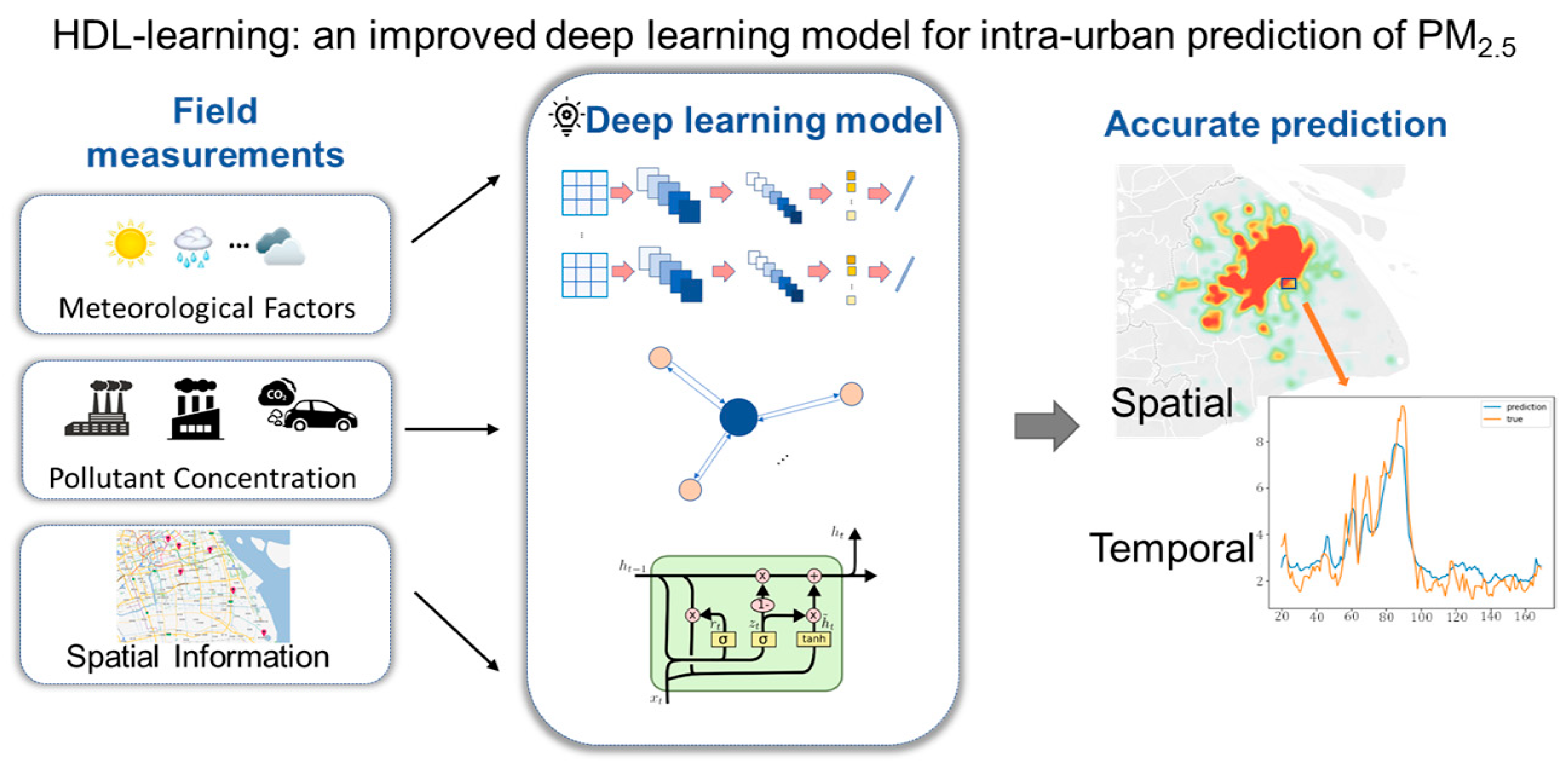
In this study, we propose a hybrid deep learning (HDL) framework (termed as HDL-learning) based on CNN-LSTM to improve the prediction of the intra-urban PM_2.5 concentration (Figure 1). The framework differs from previous studies in that, firstly, a two-dimensional CNN (2D-CNN) was applied to matrices with dimensions of data types and time series for a given station to extract nonlinear correlations of the cross-domain information and timing patterns. Subsequently, a Gaussian function was incorporated to extract the distance-based correlation of air pollutant concentrations from the given station and other stations. Finally, LSTM was designed to fully analyze and extract the long-term historical features of the input time series data to yield time series prediction data. We tested the efficiency and validity of our proposed method in the megacity of Shanghai.

2. Materials and Methods

2.1. HDL-Learning

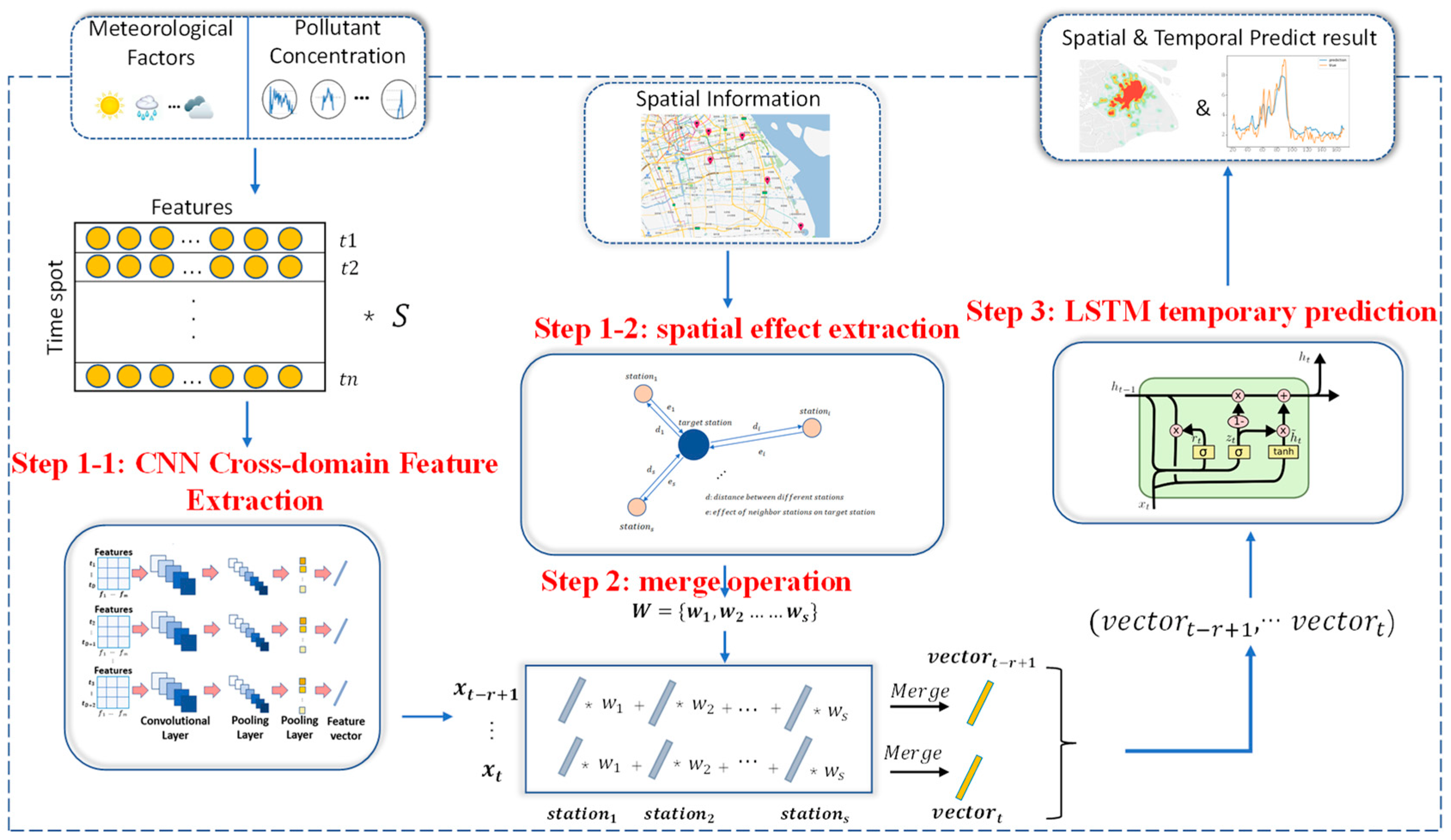
A hybrid deep learning framework called HDL-learning was developed here to predict the intra-urban variability of PM_2.5 concentrations. The overall structure of the proposed framework is illustrated in Figure 2. In the model we consider that the local PM_2.5 concentration at a given moment is influenced by three main factors: the cross-domain characteristics represented by various other environmental and weather parameters at the area, the spatial characteristics of environmental and weather parameters in the surrounding area, and the time-series characteristics generated by historical environmental parameters. For this reason, the model proposed in this study contains three components that effectively represent and integrate these three interactions. Firstly, our model uses a two-dimensional CNN network to compress and extract the cross-domain features and short-term time-dependent features of the input data (see description below) to obtain the feature vector. Meanwhile, in order to fully extract the spatial features, we calculate the weights based on the distances between other stations and the target station using a Gaussian function as a representation of the extent of environmental pollution conditions in the surrounding area on the target station. Finally, after the vector weighting calculation, the set of vectors was imported into the LSTM prediction model for time series prediction to obtain the results. The model consists of three main components: the CNN feature extraction layer, the Gaussian weight calculation layer, and the LSTM series prediction model.

2.2. CNN Feature Extraction Layer

The CNN model is one of the most researched and widely used models in the field of deep learning in recent years [23,24]. It uses local connectivity and shared weights to obtain effective representations directly from the original data by alternating between convolutional and pooling layers, automatically extracting local features of the data and building dense, complete eigenvectors.

In a CNN network, the convolution layer extracts local features of the sample data by controlling the size of the convolution kernel. The pooling layer is generally in the layer below the convolution layer and is mainly used for feature selection, reducing the feature dimension of the original data and preventing overfitting. The fully-connected layer is responsible for integrating the local features extracted earlier, and then outputting the final result. The formula for calculating each element in the feature map is:

$$x_i^{out}=f_{cov}({\displaystyle \sum _{n=0}^k{w}_n{x}_{i+n}^{in}n+b})$$

(1)

In the formula, $x_i^{out}$ is the output value and $x_{i+n}^{in}$ is the input vector; $f_{cov}\left(·\right)$ is for the activation function; $w_n$ is the weight value at position $n$; and $b$ is the bias in every calculation process.

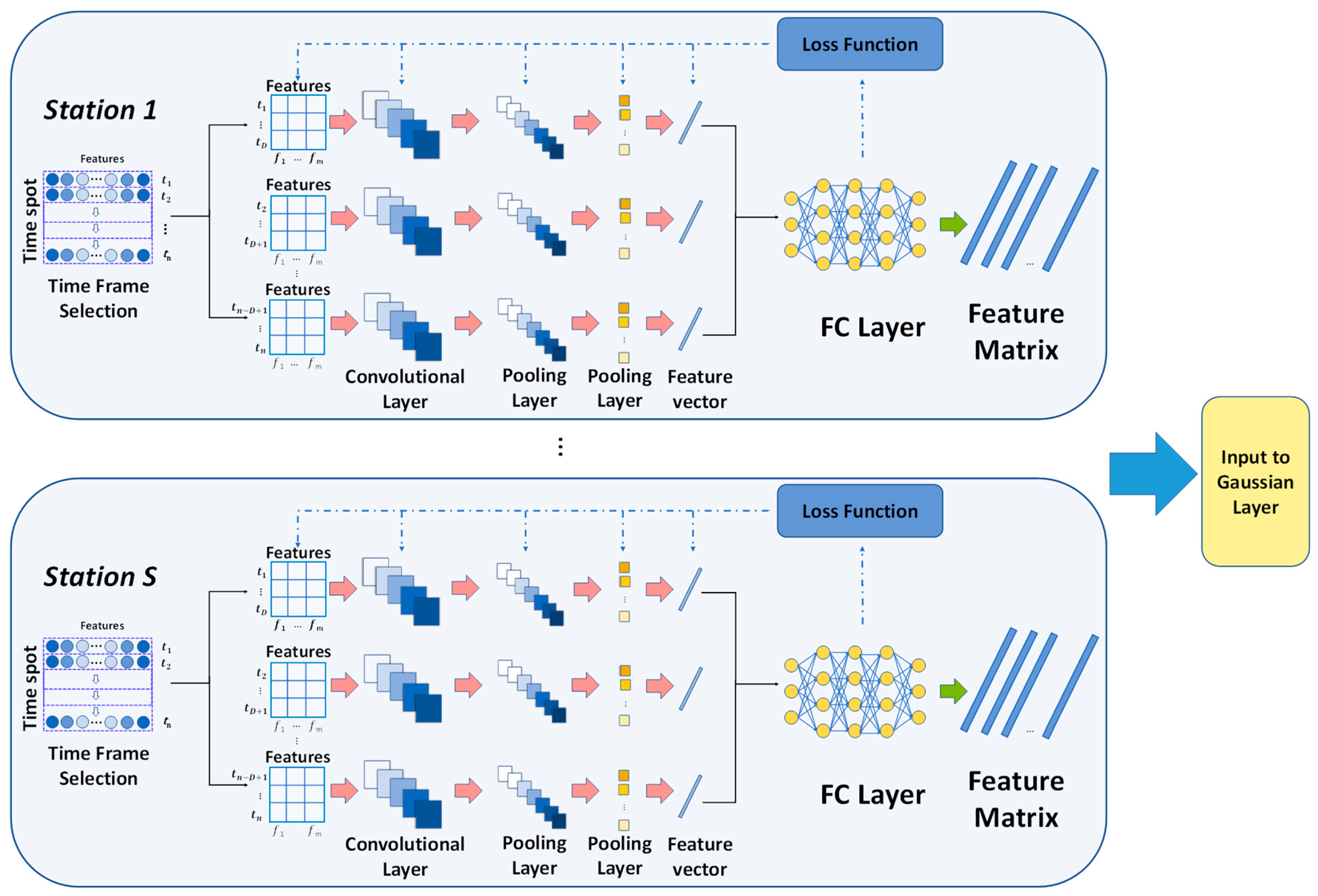
For the ability to extract data features, we use it to extract temporal features and cross-domain features for each station. We pre-set a time window of length $D$. For each moment in a time span of length $n$, m-dimensional data containing air quality and meteorological information in a time period of length $D$ centered at moment $t$ are extracted. In other words, at each moment in time $t$ in a single station, we obtain a matrix of $D\ast m$ representing the temporal and cross-domain features. Those matrixes are input into CNN for feature extraction. After convolution and pooling layers the extracted features were flattened into a 1-D array. Finally, the feature map containing the meteorological and air pollutant information of each station in every time spot was generated through the fully connected output layers, and the above steps were then applied to all stations. The structure diagram of this part is shown in Figure 3.

2.3. Gaussian Weight Calculation Layer

In each time spot, the output of the CNN layer is $s$ high dimension vectors, in which s is the number of air quality monitoring stations. Each output of $s$ vectors is calculated individually by CNN; therefore, it can precisely represent the information of low-dimension inputs.

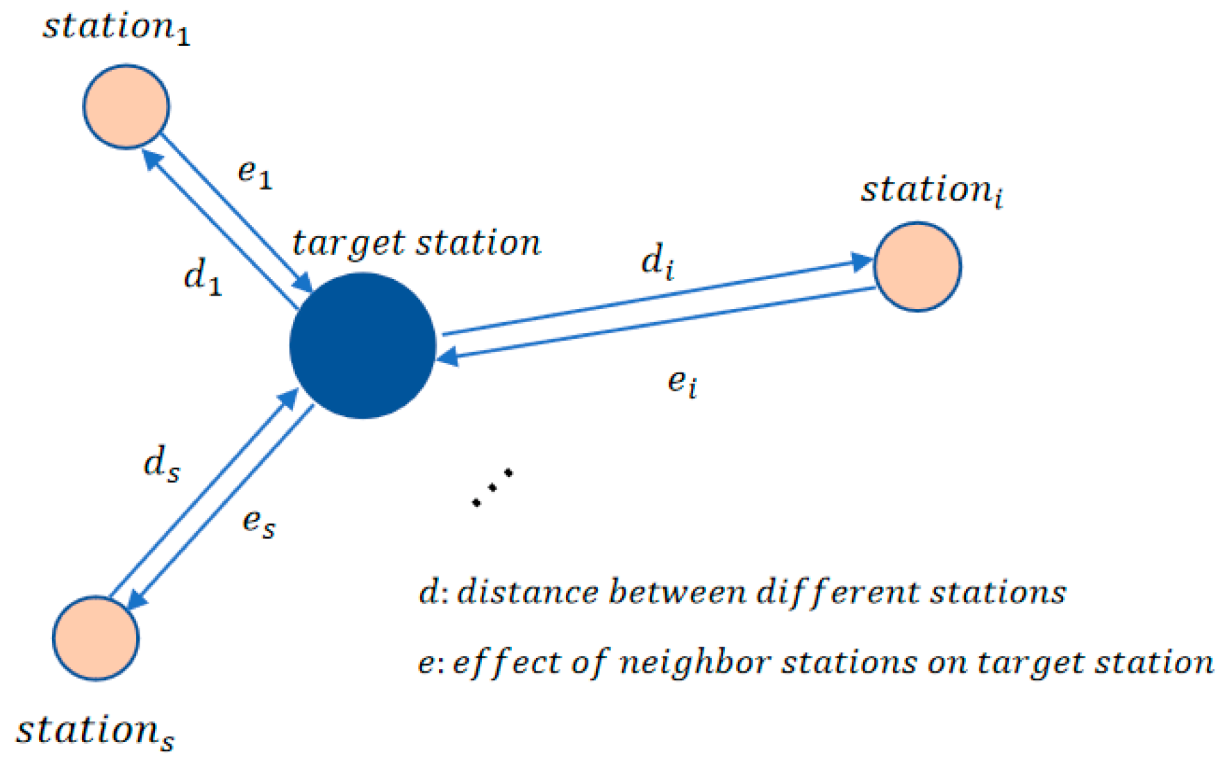
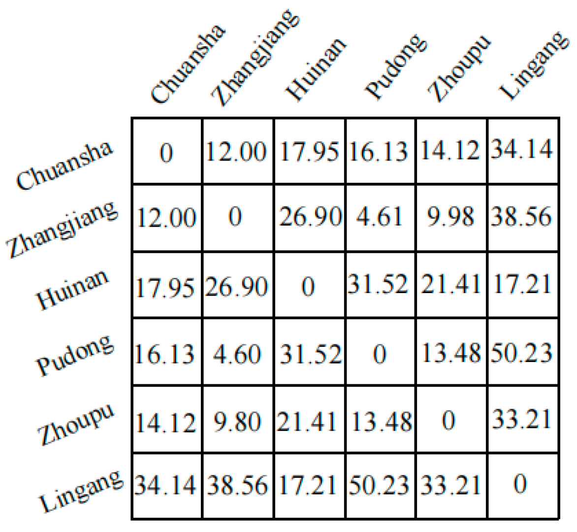
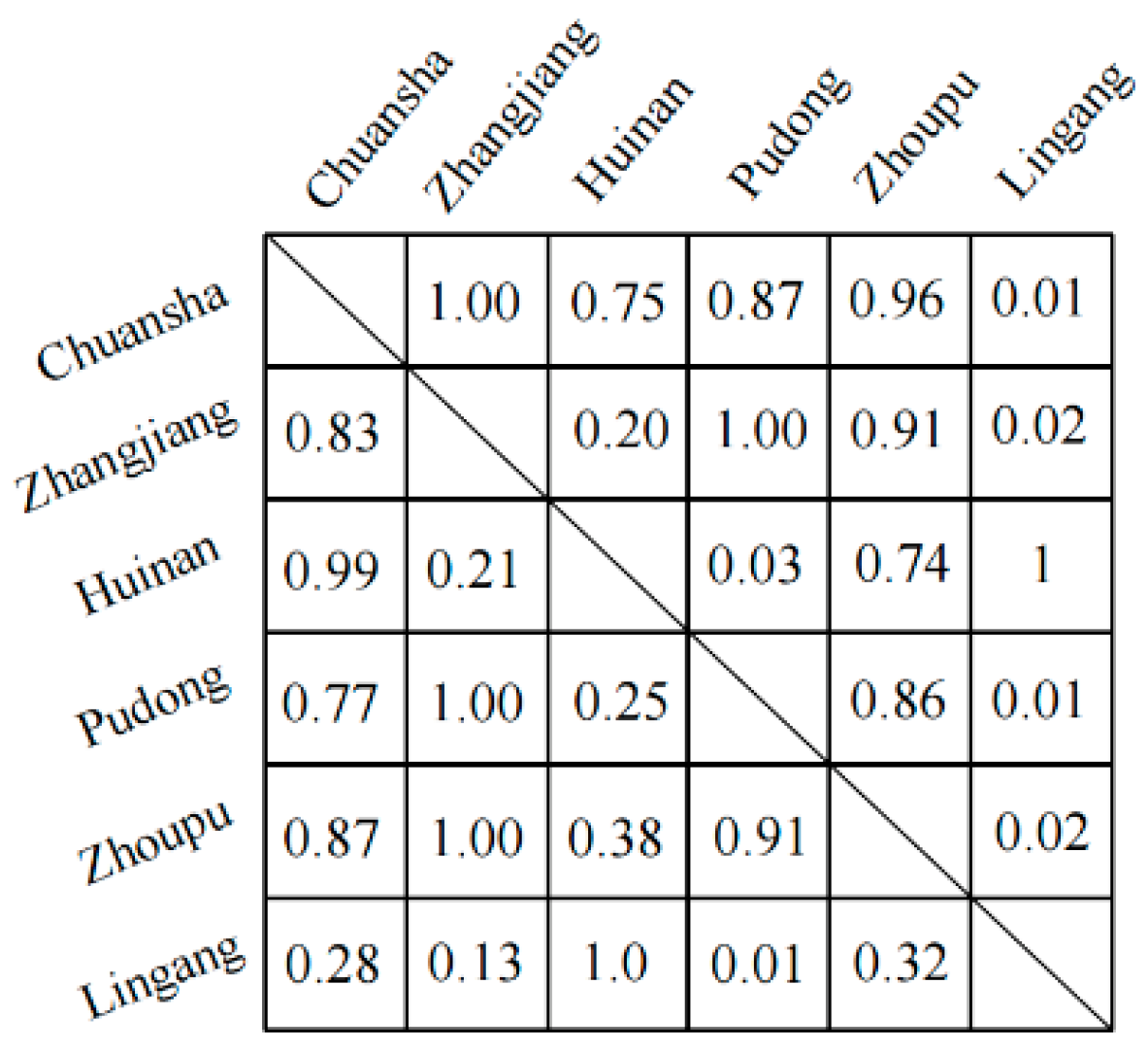
Since pollutant concentrations are affected by the spatial relationship, and the impact of pollutant concentrations in different areas on the target area follows the principle that the closer the distance, the greater the influence, we used the Gaussian model to calculate the effective degree of each neighbor station based on distance (Figure 4). 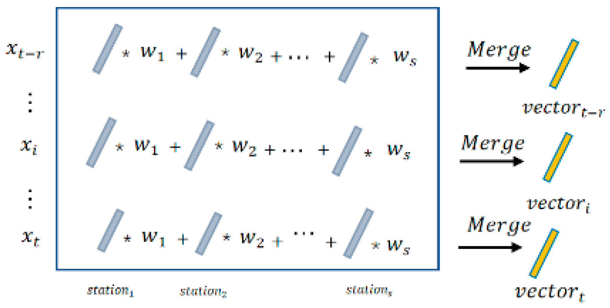In the Gaussian weight calculation layer, the station expected to be predicted is considered as target station, and distances between the other station and the target station are fed into a Gaussian function with pre-set parameters to calculate the corresponding weights which represent the spatial influence from other regions on the PM_2.5 concentration at the target station. The output of CNN for the s stations at one moment was merged into one-dimensional vectors in a time series before being inputted to LSTM.

s one-dimensional vectors were outputted during the time period ($t-r\dots , i, \dots , t$) to calculate the effective weights for each station based on its distance between target stations. The Gaussian function has the special feature that the weight is 1 when the distance between two points is the shortest among all neighbors, and tends to 0 as the distance increases. The effective weights are calculated as Equations (2) and (3).

$$w_s=A^2\times e^{-B}$$

(2)

$$A=\frac{1}{\sigma \sqrt{2\pi }},B=\frac{{(d_s-\mu )}^2}{2{\sigma }^2}$$

(3)

where $d_s$ is the geographical distance between station $s$ and the target station. The merging operation process is shown in Figure 5. In this operation, for each moment, the feature vectors of each station around the target station are multiplied and summed by the corresponding weights to obtain the merged vector. The fused vectors are then fed into the LSTM for temporal prediction.

2.4. LSTM Prediction Model

The output vector of the merge operation is then inputted to the LSTM layer. Value of $vecto{r}_{\left(t-r, \dots , t\right)}$ for $r$ hours before time $t$ are the input of LSTM time series prediction model, and the prediction target is the hourly PM_2.5 concentration value for time $t+1$. $x$ is the input and represents the dynamic time series. $W$ is for the weight matrix. C is for the memory unit. h is the hidden layer information and $b$ is the bias. The training process for LSTM is as follows:

i. The LSTM first selectively forgets some past PM_2.5 data information and other factors and we choose the σ (sigmoid) function as the activation function of the forget gate LSTM.

The value of the forget gate $f_t$ is limited between 0 to 1. As shown in Equation (4), by multiplying $f_t$ and in Equation (5), the memory unit of time t − 1 $C_{t-1}$, if the element value of $f_t$ tends to 0, it means the corresponding feature information in $C_t$ is forgotten, and if the element value of $f_t$ tends to 1, it means that the corresponding feature information is saved.

$$f_t=\sigma (W_f[h_{t-1},x_t]+b_f)$$

(4)

$$C_t^{\prime }=f_t\times C_{t-1}$$

(5)

ii. determine the new information to be stored in the storage unit.

The new information consists of two parts. The output gate $i_t$ determines the updated information and the initial updated value ${\tilde{C}}_t$ is the new candidate value vector. Equations (6) and (7) are their calculation process. By multiplying ${\tilde{C}}_t$ and $i_t$, the important feature information updated value ${\tilde{C}}_t$ is selected and stored in the memory unit.

$$i_t=\sigma (W_i[h_{t-1},x_t]+b_i)$$

(6)

$${\tilde{C}}_t=tanh(W_{\tilde{C}}[h_{t-1},x_t]+b_{\tilde{C}})$$

(7)

iii. Update the state of memory unit:

$${\tilde{C}}_t=C_t^{\prime }+i_t\times {\tilde{C}}_t$$

(8)

iv. Finally determine the prediction output information:

$$o_t=\sigma (W_o[h_{t-1},x_t]+b_o)$$

(9)

$$h_t=o_t\times tanh(C_t)$$

(10)

$h_t$ is obtained from the output gate $o_t$ and the memory unit status $C_{t }$, where the calculation method of $o_t$ is the same as that of $f_t$ and $i_t$. After that, the entire model is fine-tuned via stochastic gradient descent to attain global optimization.

LSTM adds the temporal prediction function to the model. Its inputs are one-dimensional vectors representing the real data features. Therefore, complicated and redundant calculations are avoided and reliance of the data on the temporal dimension is considered.

2.5. Experiment Setting

2.5.1. Dataset Preparation and Model Setting

China took less than a decade to establish the world’s largest air pollution monitoring network after severe haze pollution events in 2013. As of 2020, there were ~1630 state-controlled monitoring sites that required data to be released publicly. In this study, historical air quality and meteorological data (past L-hour) were used to train the model to predict hourly PM_2.5 mass concentrations (future n-hour) at a given site. To this end, we focused on Shanghai and considered air quality (including PM_2.5, PM₁₀, SO₂, NO₂, CO, and O₃; in μg m⁻³) and meteorological data (including temperature, relative humidity, wind direction, and wind speed) measured at six stations (i.e., Pudong, Zhoupu, Huinan, Chuansha, Zhangjiang, and Lingang). In total, 52,705 hourly data points were successfully obtained throughout the year 2020, in which 200-day and 166-day datasets were used for the training (adjusting relevant parameters in our models) and validation (to test the performance of our model) of our method, respectively. Details of the data we used in the study are shown in Text S1, Table S1, and Figure S1 in the Supplementary Materials. For missing data, linear spline imputation was used to interpolate and thus reconstruct a continuous and reliable dataset (For details, refer to Text S2 of the Supplementary Materials). To elucidate the correlation between pollutants and each weather variable, we did a correlation analysis of each variable prior to the formal experiment, and as a result, we found various positive and negative correlations between and within the pollutant data and weather data, with details in Text S2 and Figure S2 of the Supplementary Materials. After that, air quality and data were normalized in the range of [−1, 1] as an input to the CNN model, and wind speed/direction data were encoded and normalized as input to the subsequent network. The hyperparameters of the proposed model are contained in Text S3 of the Supplementary Materials.

The problem is formed as follows: given air pollutant data ${\left\{A{P}_s^t\right\}}_{t=1}^T$, meteorological data ${\left\{M_s^t\right\}}_{t=1}^T$, where S is the set of air quality monitoring stations $\left\{S_1, S_2, S_3,\dots ,S_n\right\}$, and T is the current timestamp, we aim to predict the AQI over the next K hours for ${\left\{PM{2.5}_S^{T+K}\right\}}_{k=1}^K$ from former air pollutant and meteorological data.

2.5.2. Inter-Comparison Parameters of Model Performance

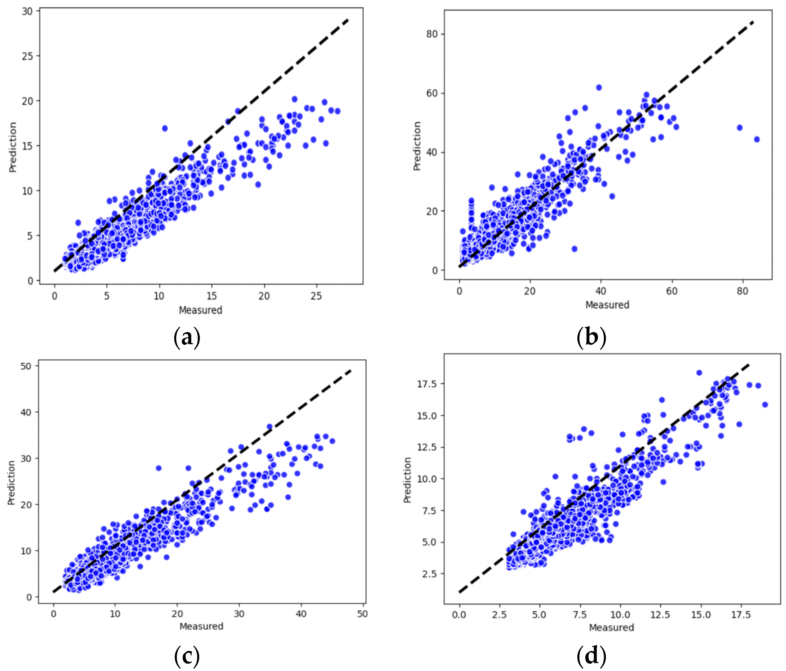
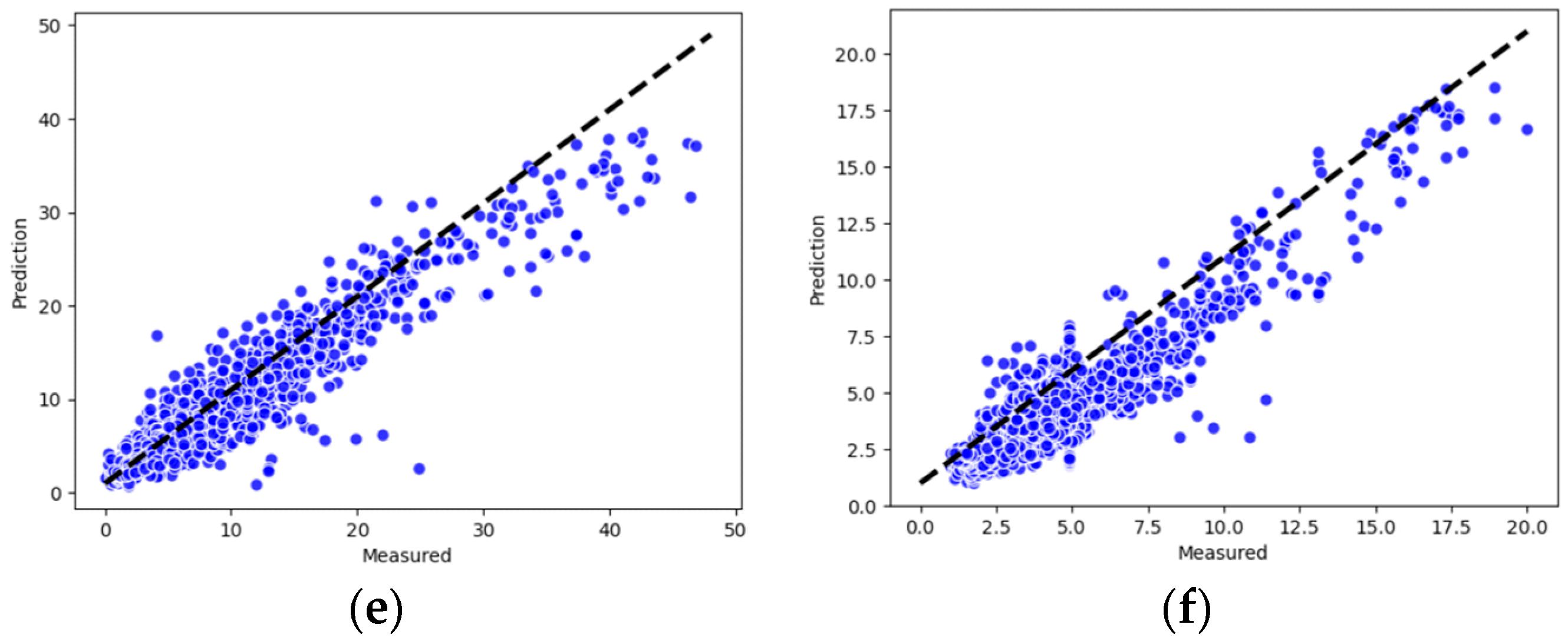
Using the same dataset as the model input, the performance of the new model proposed in this study was compared with benchmark methods used previously. Three inter-comparison parameters were used to quantitatively evaluate their performance in terms of PM_2.5 prediction.

Root mean square error (RMSE). RMSE quantifies the deviation between the predicted data and the actual data. A low value of RMSE indicates precise prediction.

Mean absolute error (MAE). MAE is the average value of absolute error, which can better reflect the actual situation of prediction error.

Determination coefficient (R²). The R² score measures how well a statistical model predicts an outcome by calculating the proportion of variance in the dependent variable that is predicted by the statistical model.

RMSE and MAE are negatively oriented, which means that lower scores imply the better performance of models, while the R² scores are positively oriented.

3. Results and Discussion

3.1. Temporal Prediction of Single Station

In this section, we first measure the performance of our method on the single station time series prediction task in order to examine the effect of temporal feature cross-domain feature extraction of HDL-learning. pollutant and meteorological data from a single station over the past 1 and 3h are input to the model to predict the pollutant PM_2.5 concentration in the next time periods. We compared our model with the widely used models LSTM, ARIMA, and SVR [25] on the prediction performance in a certain station. Figure 6 shows the fitting trends of different models, and the results are shown in

Table 1. Performance comparison of different models in a single station task.

Model	RMSE	MAE	MAAPE	R2	RWI
LSTM	1.88	1.25	27.34	0.87	0.82
ARIMA	12.26	11.92	30.67	0.77	0.71
SVR	9.30	10.35	19.43	0.81	0.78
HDL-learning	1.78	1.18	18.43	0.91	0.88

.

As can be seen from Figure 5, our model not only accurately predicts the peak, but also fits the trend of PM_2.5 concentrations more accurately. Due to the violent fluctuations in the true values, there is some error between the predicted and true values from our model, but this is generally within tolerable limits.

Compared with other methods, the proposed model has lower values in RMSE and MAE. The reduction of RMSE and MAE values indicates the reliability of our model in time-series prediction tasks.

3.2. Spatiotemporal Prediction

After evaluating the prediction performance of the proposed model in a single station, we further validate the spatiotemporal prediction efficiency of the proposed model under equal geographical weight, which means that the spatial and temporal influence of the surrounding sites on the target site are considered equally. We use the data from five stations around the target site at previous times as input and predict the PM_2.5 concentration of the target site at the next time from the perspective. This test demonstrated that by considering the spatial influence of the surrounding area, the accuracy of prediction has been improved significantly. The results are shown in Figure 7. According to the figure, our model predicted the PM_2.5 concentrations in Chuansha, Huinan, Pudong and Zhoupu with relative precision, while the fitting errors in Zhangjiang and Lingang are larger. The large fitting error for Zhangjiang may be due to data fluctuations, while the large fitting error for Lingang is due to the fact that the other stations are too far apart to learn valid spatial information.

Table 2. Performance comparison of different models on RMSE.

	Chuansha	Zhangjiang	Huinan	Pudong	Zhoupu	Lingang	Average
CNN-LSTM	1.88	3.19	2.19	0.70	1.97	2.88	2.13
CNN	21.45	12.51	10.59	6.93	35.72	11.12	16.39
ARIMA	28.20	29.42	29.95	27.01	32.62	30.25	29.57
FDN-learningW	1.80	3.18	1.79	0.69	2.15	0.82	1.73
Our model	1.78	3.17	1.25	0.70	1.94	0.84	1.61

,

Table 3. Performance comparison of different models on MAE.

	Chuansha	Zhangjiang	Huinan	Pudong	Zhoupu	Lingang	Average
CNN-LSTM	1.25	2.25	1.25	0.46	1.25	2.34	1.44
CNN	16.22	9.76	6.86	4.84	39.44	8.33	14.24
ARIMA	17.29	17.47	16.35	16.70	17.15	17.57	17.09
FDN-learningW	1.23	2.14	1.03	0.43	1.27	1.25	1.22
Our model	1.18	2.13	0.83	0.46	1.26	1.29	1.19

,

Table 4. Performance comparison of different models on R².

	Chuansha	Zhangjiang	Huinan	Pudong	Zhoupu	Lingang	Average
CNN-LSTM	0.86	0.94	0.83	0.83	0.90	0.84	0.87
CNN	0.78	0.85	0.70	0.88	0.84	0.7	0.81
ARIMA	0.65	0.70	0.69	0.73	0.76	0.672	0.70
FDN-learningW	0.95	0.89	0.93	0.86	0.91	0.87	0.90
Our model	0.98	0.95	0.99	0.94	0.94	0.91	0.95

,

Table 5. Performance comparison of different models on MAAPE.

	Chuansha	Zhangjiang	Huinan	Pudong	Zhoupu	Lingang	Average
CNN-LSTM	18.71	19.23	18.48	20.58	18.54	18.65	19.03
CNN	27.87	22.32	21.64	23.73	19.66	22.62	22.97
ARIMA	25.24	24.56	24.71	23.27	24.56	21.96	24.05
FDN-learningW	17.74	18.63	18.90	17.89	16.51	16.73	17.73
Our model	15.36	16.25	15.18	14.63	15.92	16.26	15.6

and

Table 6. Performance comparison of different models on RWI.

	Chuansha	Zhangjiang	Huinan	Pudong	Zhoupu	Lingang	Average
CNN-LSTM	0.81	0.92	0.78	0.75	0.85	0.79	0.82
CNN	0.72	0.84	0.66	0.82	0.83	0.68	0.76
ARIMA	0.64	0.67	0.66	0.72	0.74	0.62	0.68
FDN-learningW	0.92	0.84	0.89	0.81	0.86	0.82	0.86
Our model	0.92	0.91	0.93	0.90	0.89	0.85	0.9

separately present the RMSE, MAE and other comparisons of our method with baseline spatiotemporal prediction approaches including CNN-LSTM [10], CNN, ARIMA, and FDN-learningW. According to the results, on individual station prediction tasks (Pudong, Lingang), HDL-learning has slightly poorer prediction accuracy compared to FDN-learning [26], which is caused by the limitation of the CNN cross-domain information extraction layer in learning the full picture of the intrinsic relationships between pollutants. HDL-learning in general still performs huge advantages over RMSE, MAE and R² value.

The results also demonstrate that our model, with the contribution of a CNN time-series cross-domain feature extraction, achieves promising results in a geographically unweighted prediction task, and that the atmospheric dynamic and temporal patterns are well represented.

Performance of Gaussian Function Layer

Next, the Gaussian function was added in the calculation of the effective degree of each neighbor station based on distance. The distance matrix and weight matrix is indicated in Figure 8 and Figure 9.

To prove the efficiency of the Gaussian weight calculation layer on the accuracy of the PM_2.5 concentration prediction in the target station, the weighted model was compared with two other models: one is the unweighted HDL-learning measured in the previous experiment, and the other is the FDN-learning model, which also contains the geographically weighted mechanism. The results are shown in

Table 7. Performance comparison of weighted and unweighted models.

Station	HDL-Learning Unweighted		FDN-Learning		HDL-Learning Weighted
	RMSE	MAE	RMSE	MAE	RMSE	MAE
Chuansha	1.78	1.18	1.74	1.14	1.55	0.96
Zhangjiang	3.17	2.34	2.85	2.17	2.45	1.96
Huinan	1.26	0.84	1.07	0.97	1.21	0.81
Pudong	0.71	0.46	0.70	0.44	0.69	0.44
Zhoupu	1.94	1.27	1.83	1.11	1.72	1.01
Lingang	0.84	1.30	0.78	1.12	0.76	1.12
Average	1.62	1.23	1.52	1.10	1.39	1.06

.

Compared with the unweighted HDL-learning model, the results show that error metrics significantly decrease by 16% on RMSE and 15% on MAE with the incorporation of the Gaussian weight framework. Compared with FDN-learning, the performance of our model also showed advantages. The results demonstrate that with the addition of a geographical weighting layer, the prediction competence of our model was enhanced in terms of extracting geographical features between different datasets and achieving more accurate predictions, and the excellent performance of the CNN feature extraction module ensures that our model is more accurate than comparable geographic weighted models.

The actual versus predicted values of the model in the form of a scatter plot are shown in Figure 10. The plots show that most of the data points are close to the regression line and have remarkably high correlation values, indicating the good fit of our model. Therefore, the extraction of features by CNN networks and the practice of Gaussian functions to handle geolocation information are reasonable in this work.

4. Conclusions

Operating a reliable air quality forecasting model in an urban area is one of the most important tools for health protection. The accurate prediction of air quality requires accurate modelling of temporal patterns in air quality data as well as the precise analysis of interactions between pollutants and meteorological data from the cross-domain aspect. We proposed a deep learning method to accomplish this by putting together the newly designed CNN, Gaussian weight layer, and LSTM in a hierarchical architecture. The main contributions of our model are as follows:

To take spatial and temporal factors which influence the PM_2.5 concentration at station level into consideration, we leveraged data from multiple sources, including air pollutants and meteorological data from six sites covering the main area of the Pudong district. A huge improvement over previous studies was the utilization of high-frequency meteorological data and pollutant data from an official source.

We calculated weights by Gaussian function and applied them to different site data, which fully considers the spatial and temporal influence of surrounding sites on the target site. Our method can be extended to predict PM_2.5 concentration in any area.

Our innovative use of CNNs to extract cross-domain features and time-dependent features for different dimensional inputs in a single site has been shown to be accurate and efficient in experiments, with the memory function of the LSTM network explaining the dependence of the data on the time dimension. This improves the accuracy of the model’s time series prediction results.

The application of the dataset in Shanghai demonstrates the improved performance of the proposed method over classic models for next-hour air quality prediction.

The HDL-learning model was trained and validated for forecasting the air quality of six counties in Pudong, Shanghai. When compared with the baseline geographically unweighted approaches, our method showed huge improved accuracy, and it reduced the error by at least 15%. Furthermore, our model showed consistent performance in predicting instances among all counties. Therefore, the proposed method can be utilized to provide valuable support to the city administration and to trigger early warnings for adverse air quality events. Our model also has some limitations, including that the CNN network is still limited in extracting deeper variable associations and the Gaussian function is still crude in modelling the influence of the geographical location between sites. In the future, ensemble-based approaches will be explored and incorporated along with the proposed model for further improvement in the prediction performance of the proposed framework.

References

1. Yang, T.; Liu, W. Does air pollution affect public health and health inequality? Empirical evidence from China. J. Clean. Prod. 2018, 203, 43–52. [Google Scholar] [CrossRef]
2. Brauer, M.; Amann, M.; Burnett, R.T.; Cohen, A.; Dentener, F.; Ezzati, M.; Henderson, S.B.; Krzyzanowski, M.; Martin, R.V.; Van Dingenen, R.; et al. Exposure Assessment for Estimation of the Global Burden of Disease Attributable to Outdoor Air Pollution. Environ. Sci. Technol. 2012, 46, 652–660. [Google Scholar] [CrossRef] [PubMed] [Green Version]
3. Bartell, S.M.; Longhurst, J.; Tjoa, T.; Sioutas, C.; Delfino, R.J. Particulate Air Pollution, Ambulatory Heart Rate Variability, and Cardiac Arrhythmia in Retirement Community Residents with Coronary Artery Disease. Environ. Health Perspect. 2013, 121, 1135–1141. [Google Scholar] [CrossRef] [PubMed]
4. Shou, Y.K.; Huang, Y.L.; Zhu, X.Z.; Liu, C.Q.; Hu, Y.; Wang, H.H. A review of the possible associations between ambient PM2.5 exposures and the development of Alzheimer’s disease. Ecotoxicol. Environ. Saf. 2019, 174, 344–352. [Google Scholar] [CrossRef] [PubMed]
5. Fu, P.F.; Guo, X.B.; Cheung, F.M.H.; Yung, K.K.L. The association between PM2.5 exposure and neurological disorders: A systematic review and meta-analysis. Sci. Total Environ. 2019, 655, 1240–1248. [Google Scholar] [CrossRef]
6. Athira, V.; Geetha, P.; Vinayakumar, R.; Soman, K. Deepairnet: Applying recurrent networks for air quality prediction. Procedia Comput. Sci. 2018, 132, 1394–1403. [Google Scholar]
7. Ma, J.; Ding, Y.; Cheng, J.C.; Jiang, F.; Wan, Z. A temporal-spatial interpolation and extrapolation method based on geographic Long Short-Term Memory neural network for PM2.5. J. Clean. Prod. 2019, 237, 117729. [Google Scholar] [CrossRef]
8. Tong, Y.; Yu, Y.; Hu, X.; He, L. Performance analysis of different kriging interpolation methods based on air quality index in wuhan. In Proceedings of the 2015 Sixth International Conference on Intelligent Control and Information Processing (ICICIP), Wuhan, China, 26–28 November 2015; pp. 331–335. [Google Scholar]
9. Zhou, G.Q.; Xu, J.M.; Xie, Y.; Chang, L.Y.; Gao, W.; Gu, Y.X.; Zhou, J. Numerical air quality forecasting over eastern China: An operational application of WRF-Chem. Atmos. Environ. 2017, 153, 94–108. [Google Scholar] [CrossRef]
10. Wu, Q.; Lin, H. A novel optimal-hybrid model for daily air quality index prediction considering air pollutant factors. Sci. Total Environ. 2019, 683, 808–821. [Google Scholar] [CrossRef]
11. Kim, Y.; Fu, J.S.; Miller, T.L. Improving ozone modeling in complex terrain at a fine grid resolution: Part I—Examination of analysis nudging and all PBL schemes associated with LSMs in meteorological model. Atmos. Environ. 2010, 44, 523–532. [Google Scholar] [CrossRef]
12. Bray, C.D.; Battye, W.; Aneja, V.P.; Tong, D.; Lee, P.; Tang, Y.H.; Nowak, J.B. Evaluating ammonia (NH3) predictions in the NOAA National Air Quality Forecast Capability (NAQFC) using in-situ aircraft and satellite measurements from the CalNex2010 campaign. Atmos. Environ. 2017, 163, 65–76. [Google Scholar] [CrossRef]
13. Baklanov, A.; Mestayer, P.G.; Clappier, A.; Zilitinkevich, S.; Joffre, S.; Mahura, A.; Nielsen, N.W. Towards improving the simulation of meteorological fields in urban areas through updated/advanced surface fluxes description. Atmos. Chem. Phys. 2008, 8, 523–543. [Google Scholar] [CrossRef] [Green Version]
14. Dong, C.; Loy, C.C.; He, K.; Tang, X. Image Super-Resolution Using Deep Convolutional Networks. IEEE Trans. Pattern Anal. Mach. Intell. 2016, 38, 295–307. [Google Scholar] [CrossRef] [Green Version]
15. Hao, X.; Zhang, G.; Ma, S. Deep Learning. Int. J. Semant. Comput. 2016, 10, 417–439. [Google Scholar] [CrossRef] [Green Version]
16. Ong, B.T.; Sugiura, K.; Zettsu, K. Dynamically pre-trained deep recurrent neural networks using environmental monitoring data for predicting PM2.5. Neural Comput. Appl. 2016, 27, 1553–1566. [Google Scholar] [CrossRef] [Green Version]
17. Li, X.L.; Luo, A.R.; Li, J.G.; Li, Y. Air Pollutant Concentration Forecast Based on Support Vector Regression and Quantum-Behaved Particle Swarm Optimization. Environ. Model. Assess. 2019, 24, 205–222. [Google Scholar] [CrossRef]
18. Kuremoto, T.; Kimura, S.; Kobayashi, K.; Obayashi, M. Time series forecasting using a deep belief network with restricted Boltzmann machines. Neurocomputing 2014, 137, 47–56. [Google Scholar] [CrossRef]
19. Quang, D.; Xie, X.H. DanQ: A hybrid convolutional and recurrent deep neural network for quantifying the function of DNA sequences. Nucleic Acids Res. 2016, 44, 6. [Google Scholar] [CrossRef] [Green Version]
20. Pak, U.; Kim, C.; Ryu, U.; Sok, K.; Pak, S. A hybrid model based on convolutional neural networks and long short-term memory for ozone concentration prediction. Air Qual. Atmos. Health 2018, 11, 883–895. [Google Scholar] [CrossRef]
21. Karim, F.; Majumdar, S.; Darabi, H.; Chen, S. LSTM Fully Convolutional Networks for Time Series Classification. IEEE Access 2018, 6, 1662–1669. [Google Scholar] [CrossRef]
22. Huang, C.J.; Kuo, P.H. A Deep CNN-LSTM Model for Particulate Matter (PM2.5) Forecasting in Smart Cities. Sensors 2018, 18, 22. [Google Scholar] [CrossRef] [PubMed] [Green Version]
23. Sun, Y.; Wang, X.G.; Tang, X. Deep Learning Face Representation from Predicting 10,000 Classes. In Proceedings of the 27th IEEE Conference on Computer Vision and Pattern Recognition (CVPR), Columbus, OH, USA, 23–28 June 2014; pp. 1891–1898. [Google Scholar]
24. Krizhevsky, A.; Sutskever, I.; Hinton, G.E. ImageNet classification with deep convolutional neural networks. Commun. ACM 2017, 60, 84–90. [Google Scholar] [CrossRef] [Green Version]
25. Murillo-Escobar, J.; Sepulveda-Suescun, J.P.; Correa, M.A.; Orrego-Metaute, D. Forecasting concentrations of air pollutants using support vector regression improved with particle swarm optimization: Case study in Aburra Valley, Colombia. Urban Clim. 2019, 29, 100473. [Google Scholar] [CrossRef]
26. Zou, G.J.; Zhang, B.; Yong, R.H.; Qin, D.M.; Zhao, Q. FDN-learning: Urban PM2.5-concentration Spatial Correlation Prediction Model Based on Fusion Deep Neural Network. Big Data Res. 2021, 26, 100269. [Google Scholar] [CrossRef]
Figure 1. TOC art.
Atmosphere 14 00599 g001
Figure 2. Architecture overview of the HDL-learning framework.
Atmosphere 14 00599 g002
Figure 3. CNN structure of the model.
Atmosphere 14 00599 g003
Figure 4. Spatial effect of neighbors.
Atmosphere 14 00599 g004
Figure 5. Vector merge operation.
Atmosphere 14 00599 g005
Figure 6. Fitting trends of the different models. (a) LSTM; (b) ARIMA; (c) SVR; (d) HDL-learning.
Atmosphere 14 00599 g006
Figure 7. Fitting trends of different stations: (a) Chaunsha; (b) Zhangjiang; (c) Huinan; (d) Pudong; (e) Zhoupu; (f) Lingang.
Atmosphere 14 00599 g007aAtmosphere 14 00599 g007b
Figure 8. The distance matrix of six counties.
Atmosphere 14 00599 g008
Figure 9. The weight matrix of six counties.
Atmosphere 14 00599 g009
Figure 10. Scatter plot showing the model performance over several locations in Shanghai. (a) Chuansha corr = 0.873; (b) Zhangjiang corr = 0.891; (c) Huinan corr = 0.954; (d) Pudong corr = 0.965; (e) Zhoupu corr = 0.948; (f) Lingang corr = 0.932.
Atmosphere 14 00599 g010aAtmosphere 14 00599 g010b