Article

Air Quality Impact Estimation Due to Uncontrolled Emissions from Capuava Petrochemical Complex in the Metropolitan Area of São Paulo (MASP), Brazil

by
Monique Silva Coelho
*,
Daniel Constantino Zacharias
,
Tayná Silva de Paulo
,
Rita Yuri Ynoue
and
Adalgiza Fornaro
Departamento de Ciências Atmosféricas (DCA), Instituto de Astronomia, Geofísica e Ciências Atmosféricas, Universidade de São Paulo (IAG-USP), Sao Paulo 05508-090, Brazil
*
Author to whom correspondence should be addressed.
Atmosphere 2023, 14(3), 577; https://doi.org/10.3390/atmos14030577
Submission received: 29 January 2023 / Revised: 7 March 2023 / Accepted: 10 March 2023 / Published: 17 March 2023
(This article belongs to the Special Issue Urban Air Quality Modelling)

Abstract

:
In the second quarter of 2021, the companies at the Capuava Petrochemical Complex (CPC, Santo André, Brazil) carried out a 50-day scheduled shutdown for the maintenance and installation of new industrial equipment. This process resulted in severe uncontrolled emissions of particulate matter (PM) and volatile organic compounds (VOCs) in a densely populated residential area (~3400 inhabitants/km2). VOCs can be emitted directly into the atmosphere in urban areas by vehicle exhausts, fuel evaporation, solvent use, emissions of natural gas, and industrial processes. PM is emitted by vehicle exhausts, mainly those powered by diesel, industrial processes, and re-suspended soil dust, in addition to that produced in the atmosphere by photochemical reactions. Our statistical analyses compared the previous (2017–2020) and subsequent (2021–2022) periods from this episode (April–May 2021) from the official air quality monitoring network of the PM10, benzene, and toluene hourly data to improve the proportion of this period of uncontrolled emissions. Near-field simulations were also performed to evaluate the dispersion of pollutants of industrial origin, applying the Gaussian plume model AERMOD (steady-state plume model), estimating the concentrations of VOC and particulate matter (PM10) in which the population was exposed in the region surrounding the CPC. The results comparing the four previous years showed an increase in the mean concentrations by a factor of 2 for PM10, benzene, and toluene, reaching maximum values during the episode of 174 µg m−3 (PM10), 79.1 µg m−3 (benzene), and 58.7 µg m−3 (toluene). Meanwhile, these higher concentrations continued to be observed after the episode, but their variation cannot be fully explained yet. However, it is worth highlighting that this corresponds to the post-pandemic period and the 2022 data also correspond to the period from January to June, that is, they do not represent the annual variation. A linear correlation indicated that CPC could have been responsible for more than 60% of benzene measured at the Capuava Air Quality Station (AQS). However, the PM10 behavior was not fully explained by the model. AERMOD showed that the VOC plume had the potential to reach a large part of Mauá and Santo André municipalities, with the potential to affect the health of more than 1 million inhabitants.

1. Introduction

The metropolitan area of São Paulo (MASP) is among the largest urban agglomerations in the world with more than 22 million inhabitants. The official inventory of air pollutant sources showed that more than 7 million vehicles were responsible for the emission of 24.9 (72.8%), 48.3 (64.9%), and 1.22 (40%) kton per year of hydrocarbons (HC) and particulate matter (PM), respectively, in 2020 [1]. On the other hand, despite being less intense, industrial sources and fuel-based storage were responsible for the emission of 9.3 (27.2%) and 3.6 (10%) kton per year of HC and PM, respectively [1]. In the southeast region of MASP there are seven important municipalities, known as the ABC region, with more than 2.8 million inhabitants; this is where Capuava Petrochemical Complex (CPC), the most important industrial complex of MASP, is located.
The CPC (lat. −23.6404, lon. −46.4843, Figure 1, in ABC region) stands out among the industrial emissions, contributing to the deterioration of air quality in that region [2,3,4]. The CPC is composed of the Capuava Oil Refinery (RECAP), Braskem S.A. and other industries, in a range of ~8.5 km2 inside a densely populated (~3400 inhabitants/km2) urban area.
This complex produces gasoline, diesel (S-10), liquefied petroleum gas (LPG) ethylene, propylene, and polyethylene from the distillation of naphtha, as well as fertilizers and various intermediates with the capacity to process about 53,000 barrels of oil per day [4,5]. Braskem S.A. and RECAP are close (~1.0 km) to the Capuava Air Quality Station (AQS) (Figure 1) that has been monitoring benzene and toluene since 2017, and they are representative of the urban air measurement, including the presence of the CPC [6].
On 14 April 2021, the Environmental Agency of São Paulo State (CETESB) announced that the companies Braskem S.A. and Capuava Refinery (RECAP), located inside the CPC, were fined for improper emissions that reached several neighborhoods, causing discomfort and hundreds of public complaints [1]. This was a consequence of general maintenance; for instance, the flare had been turned off for cleanup during April and May 2021 (approximately 50 days), causing the most acute period of odorous substance emission from 4 to 11 April 2021 [7]. The effects registered, such as headaches and nausea, reported by residents correspond to the classical knowledge of exposure to VOCs [8,9].
VOCs can be emitted directly into the atmosphere, in urban areas, by vehicle exhausts, fuel evaporation, solvent use, emissions of natural gas, and industrial processes. PM is emitted by vehicle exhausts, mainly those powered by diesel, industrial processes, and re-suspended soil dust, in addition to that produced in the atmosphere by photochemical reactions [2,10]. VOCs have been widely studied around the world, both to assess their role in the formation of secondary pollutants, such as ozone (O3) and secondary organic aerosol (SOA), and to determine health and environmental risks, due to their toxicity [10,11,12,13,14,15,16]. PM10 and PM2.5 concentrations higher than those of the World Health Organization (WHO) guidelines have been observed worldwide, as well as in MASP. Additionally, the human exposure to these particles has been evaluated as one of the top ten environmental health risk factors [17,18,19].
A recent study has provided a detailed analysis of 35 non-methane hydrocarbons (NMHC) measured near the CPC area [2], including alkanes (C6-C11), aromatics (C6-C10), and alkenes (cis/trans-2-hexene). The field campaign, which took place from 2016 to 2017, depicted the most abundant compounds near CPC as being toluene (1.5 ± 1.1 ppbv), cis-2-hexene (1.4 ± 1.9 ppbv), benzene (0.55 ± 0.66 ppbv), and m+p-xylene (0.58 ± 0.3 ppbv). Furthermore, the observations showed higher NMHC concentrations (by a factor of 2) at the site near the industrial complex when compared to the one located at the University Federal of the ABC (UFABC), where vehicular traffic dominates the pollutant emissions. The aromatics were the most abundant, reaching 56–58% among the evaluated hydrocarbons [2]. The evaluation of correlations and ratios of benzene, toluene, ethylbenzene, and xylenes (BTEX), all aromatic hydrocarbons that represent a significant fraction of VOCs [20], showed that in addition to the industrial influence around CPC, vehicular contributions were also observed [2]. The comparison with other industrial areas worldwide showed a similar NMHC profile as that in Japan and the United States of America (USA), suggesting the presence of similar emission sources [2,21,22].
The lifetime cancer risk for Capuava was estimated by comparing the risk among BTEX compounds. Benzene presented the highest probability of cancer risk, six times higher than the value recommended by the United States Environmental Protection Agency (US EPA) for people who spend most of their time at work or who live in Santo André and Mauá, especially in the CPC’s vicinity [2].
The biomonitoring of air pollution in Santo André city has evidenced the highest concentrations of pollutants in the vicinity of CPC, in comparison to the areas which are not under the influence of the industries [4]. In the same place, one study identified statistically significant effects between PM10 levels and hospitalizations of elderly patients associated with congestive heart failure [3]. Another study investigated the air pollution relationship with blood pressure alterations and concluded that traffic controllers working outdoor shifts in Santo André presented higher blood pressure during exposure to local pollutants [23]. In addition, atmospheric pollutants in the CPC area seem to be the highest risk factor for primary hypothyroidism in children and adults, but a considerable increase in the incidence of this disease was observed in residents in the proximity of CPC [24,25,26].
Since the 1990s, the CETESB AQS has been monitoring O3, nitrogen dioxide (NO2), sulfur dioxide (SO2), inhalable particles (PM10), fine particulate matter (PM2.5), and carbon monoxide (CO) concentrations in MASP. Frequent exceedances of WHO guidelines [19] for O3 and PM2.5 have been reported in the CPC area. In 2017, CETESB began the automatic hourly monitoring of benzene and toluene at Capuava AQS, which is the only station that monitors these compounds in this area, representing the influence of industrial emissions in the region.
Capuava had the highest annual average concentrations for benzene when compared with the CETESB AQS in the other large industrial areas such as the cities of Cubatão and Paulinia. The benzene annual averages in recent years were as follows: 2017: 2.8 µg m−3; 2018: 1.6 µg m−3; 2019: 2.8 µg m−3; and 2020: 2.6 µg m−3, and toluene annual averages were as follows: 2017: 5.7 µg m−3; 2018: 5.0 µg m−3; 2019: 5.0 µg m−3; and 2020: 3.9 µg m−3 at Capuava AQS [6]. At the same station, for 2020, aldehydes were also monitored. The averages observed for formaldehyde and acetaldehyde were 4.3 and 3.2 µg m−3, respectively, and their maximum values were 21.9 and 15.3 µg m−3, respectively [6].
The health effects caused by the presence of industrial emissions in the region have already been demonstrated in previous studies [3,4,23,24,25,26], and air quality stations have been showing that pollutant concentrations constantly exceed the Brazilian air quality standards [6]. In MASP, where vehicular emissions have been decreasing in recent decades [17], it is necessary to evaluate other sources of air pollution, such as industrial emissions and their implications in air quality degradation, mainly in acute episodes, as we discuss in the present study.
Despite the few studies developed in the great ABC region, the evidence of the air pollution health effects, and the fact that local industrial emissions are an additional source of VOCs in MASP, little is known about CPC emissions that result in odor and soot episodes denounced by the media in that neighborhood. In this paper, we provide a detailed analysis of the benzene, toluene, and PM10 concentrations measured in the Capuava AQS from 2017 to 2022. We provide statistical analyses from these Capuava AQS hourly data and near-field plume modeling (AERMOD) results, improving the knowledge about the contribution of uncontrolled emissions from CPC during the episode and their environmental impacts.

2. Materials and Methods

2.1. Gaussian Plume Model (AERMOD)

In the state of the art of regulatory models, AERMOD (steady-state plume model) is recommended for short-range impact, <50 km [27]. On the other hand, CALPUFF (California Puff: non-steady-state puff dispersion model) [28] and FLEXPART (flexible particle dispersion model) [29] are suggested for longer ranges (>50 km), while CMAQ (community multiscale air quality) [30] is developed for photochemistry modeling, and HYSPLIT (hybrid single-particle Lagrangian integrated trajectory) is designed for complex dispersion and deposition simulation [31].
AERMOD is a Gaussian plume model used to simulate near-field pollutant dispersion from industrial sources. It is based on the planetary boundary layer turbulence structure from Monin–Obukhov similarity theory, and it includes the treatment of both surface and elevated sources, as well as simple and complex terrain [32]. AERMOD has been tested in several arrangements: industrial and agricultural facilities, with high-resolution land use modeling episodes, or multiple years spent conducting environmental impact assessments. It has been estimating the levels of exposure to gases and PM of the population living close to the installations [33,34,35,36,37,38,39,40]. In the regulatory applications as environmental impact assessments (EIAs), AERMOD simulations cover the most recent 5-year period of atmospheric data. A worst-case scenario was applied, estimating the highest concentrations that can be found in an area, with five years of recurrence [35].
Different studies have been developed using this model, such as the dispersion of pollutants from thermal power plants [33] and the evaluation of atmospheric vehicle pollution [34]; atmospheric dispersion and the deposition of ammonia [35]; laboratory dispersion experiments to improve dispersion model performance [36]; modeling CO2 and NO2 emission from an industrial stack [37], and oil refinery odor emission rates estimated via reverse dispersion modeling [40].
The substantial simulation period (five years) helps to ensure the inclusion of the worst-case scenario in the modeling period [35]. However, situations with loss of emission control, as occurred in Capuava in 2021, are not provided in the EIAs and can generate higher concentrations, causing harmful acute effects among the population health.
The Lakes Environmental © AERMOD v. 10.0.1 was used to model the dispersion of CPC emission of pollutants (VOC and PM) for the episode period to predict ground-level pollutant concentrations in the stable boundary layer (SBL) and in a horizontal direction in the convective boundary layer (CBL) [39]. AERMOD requires source data (source geometry, pollutant emission rates, emitted gas stream temperature, and flow rate (Table S2)), topographical data for sources and receptors, and meteorological data (Table S3) as inputs and outputs of ambient pollutant concentrations at receptors. Two preprocessors called AERMAP and AERMET convert raw topographical and meteorological data to the readable format for AERMOD through two separate runs before dispersion modeling runs [40,41].
The terrain was pre-processed using AERMAP and SRTM1/SRTM3 data. The Shuttle Radar Topography Mission (SRTM, [41]) digital elevation data are part of an international research effort that obtained digital elevation models on a near-global scale, provided by National Aeronautics and Space Administration (NASA) at a resolution of 1 arc-second (approximately 30 m). The land use was pre-processed using NLCD 2001–2016 land use codes (National Land Cover Database, Wickham et al., 2021) with 1 km GLCC data (global land cover characterization). GLCC is a series of global land cover classification datasets that are based primarily on the unsupervised classification of 1 km AVHRR (advanced very-high-resolution radiometer) and 10-day NDVI (normalized difference vegetation index) composites (USGS, 2021). GLCC data were post-processed using 2021 Google Earth satellite images and WebLakes Land User Creator to increase the horizontal resolution until 1 arc-second (approximately 30 m).
Emission rates, buildings, stacks, and industrial maps were obtained via the EIA and environmental licenses from CETESB (Braskem process number 16/01562/04, license 16011156, dated 15 March 2021, and RECAP process number 16/01566/04, license 16011084, dated 4 January 2021) due to the law on access to information, privacy, and health research in Brazil (Federal Law n. 12.527/2011). In addition, using the industrial map, we visually identified the tanks in order to insert an estimation of fugitive emissions. We made the following considerations: height and diameter of each tank and VOC flow rate of 0.5 m s−1. Braskem and RECAP’s EIA were used in the industrial tridimensional modeling (Figure 2, KML data are also available in the Supplementary Material).

2.2. Air Quality Data Analysis

The available data of hourly pollutants (PM10, benzene, and toluene), wind direction, and wind speed from Capuava AQS (https://cetesb.sp.gov.br/ar/qualar/, accessed on 10 January 2023) were analyzed from 2017 to 2022. Statistical analyses of data were performed using R statistical software—open-air package (https://www.r-project.org/, accessed on 18 June 2022 [42])—which has been used extensively in different studies, such as elements inside PM2.5 in urban areas [43], the analysis of air pollution on a roadside [44], air pollution and biomass burning [45], and the study of different VOC sources [10,46,47].
The normalization in the diurnal profiles enables the comparison among variables on contrasting scales. The variables were divided by their mean values, which helped compare the diurnal trends for the compounds evaluated in the present study [43,48]. Additionally, pollutant concentrations with values higher than (mean + 3 × (standard deviation)) were considered to be outliers in the data validation and were excluded from boxplot analyses. To identify potential contributions from the sources, we used the polar annulus function, which is a graphical resource that provides temporal variation in concentrations for each compound according to wind direction. The code and major information are available in the open-air package manual [42].
The Pearson correlation coefficient between modeled data (AERMOD) and Capuava AQS data was analyzed to provide a statistical evaluation for the AERMOD performance [48]. The Pearson correlation is normally used to reflect the linear correlation and it demonstrates the contribution from similar emission sources [12,49].

3. Results and Discussions

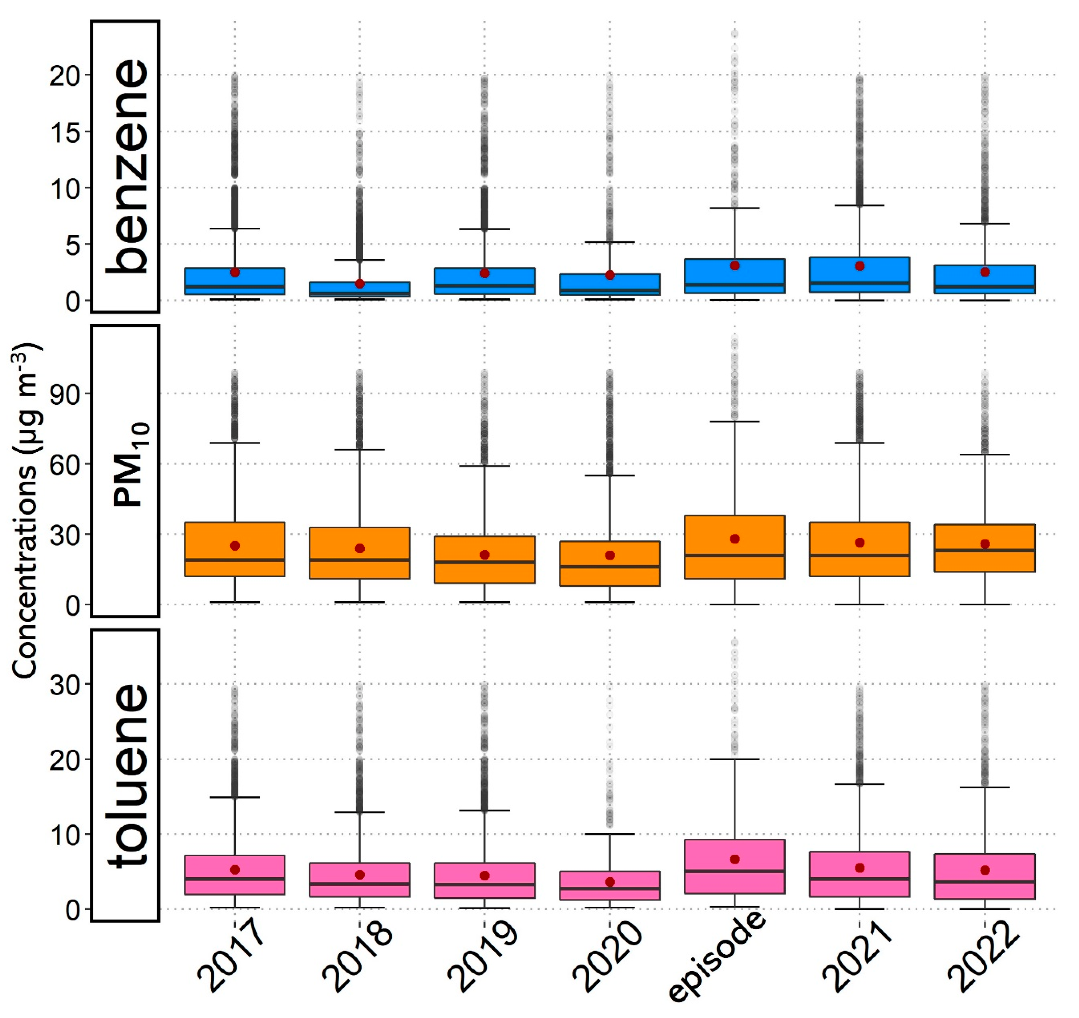
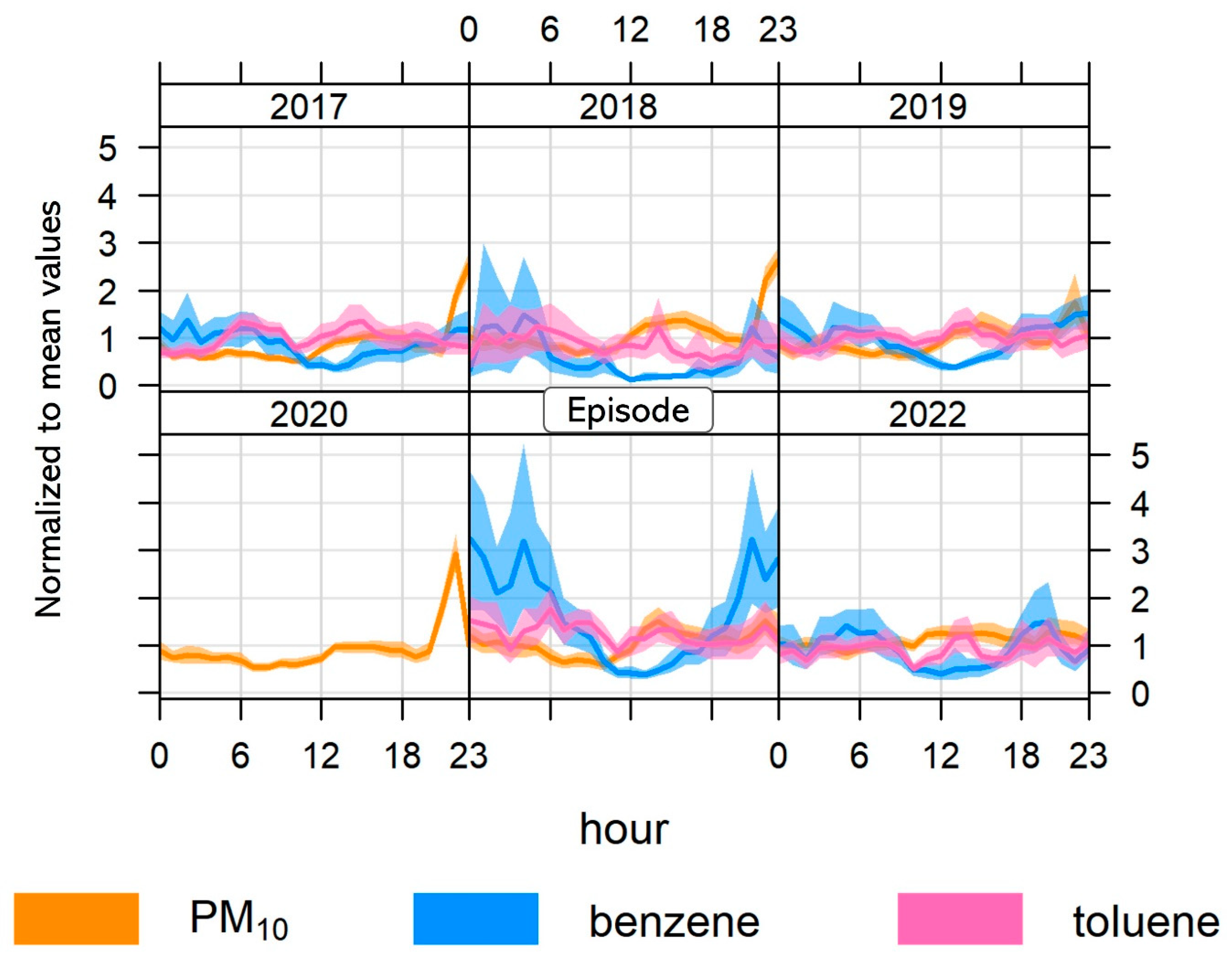
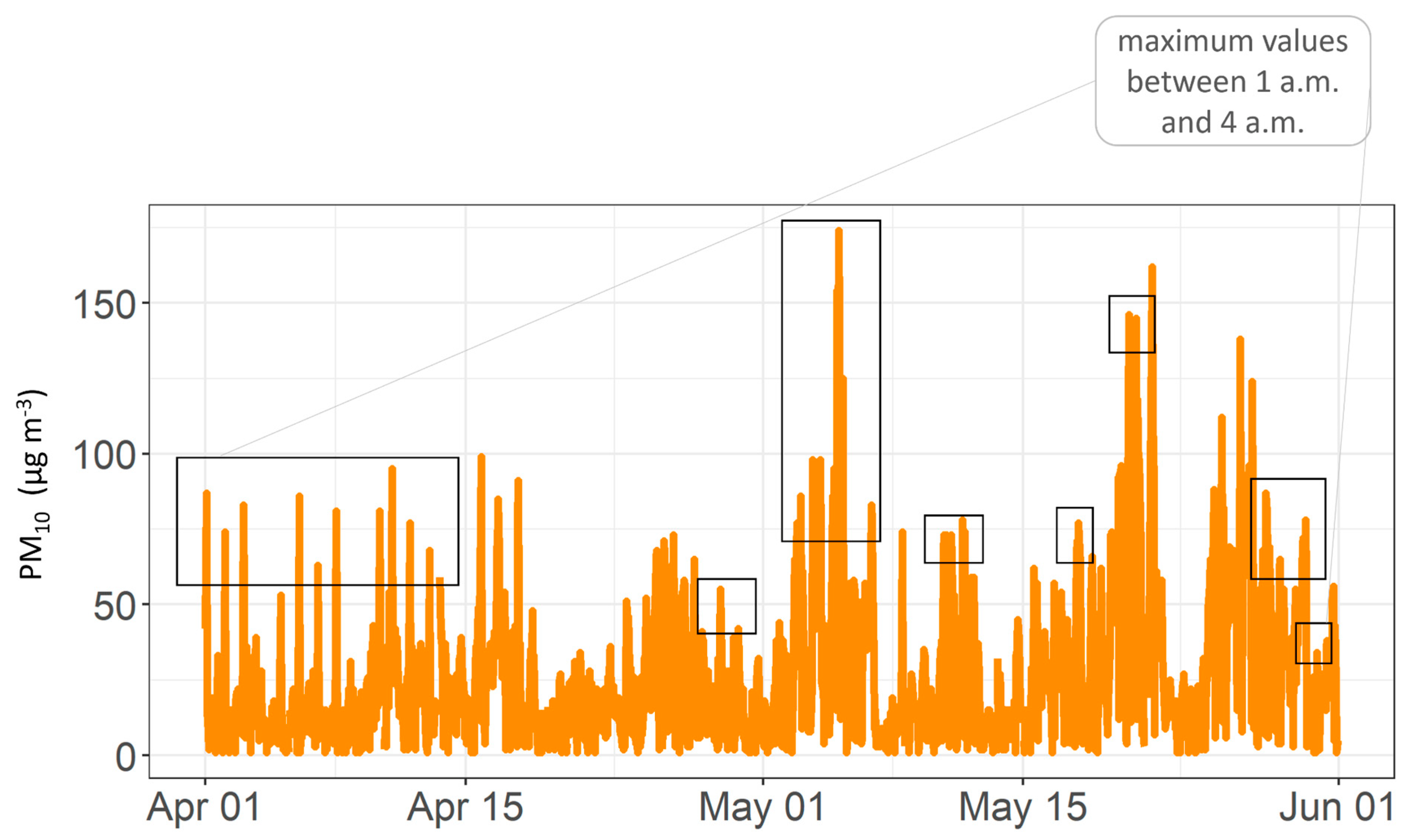
3.1. Air Quality Data

The episode period of uncontrolled emissions (April–May 2021) was statistically analyzed by comparing the previous (2017–2020) and the subsequent (2021–2022) periods (Figure 3 and Table S1). The annual averages at Capuava AQS varied from 21.6 µg m−3 to 29.4 µg m−3 for PM10, from 1.5 µg m−3 to 4.2 µg m−3 for benzene, and from 3.7 µg m−3 to 5.9 µg m−3 for toluene (Figure 3 and Table S1). It is possible to determine the variability of the data through the interquartile intervals between the first and third quartile. Thus, the highest variability and values of PM10, benzene, and toluene happened with the highest amplitude, as well as the average concentrations reaching 29.3 µg m−3 (PM10), 4.6 µg m−3 (benzene), and 7.1 µg m−3 (toluene) in this episode period (Figure 3 and Table S1).
When we compare the mean concentrations between the previous period (2017–2020) and episode (April–May 2021), an increase by a factor of 1.95, 1.53, and 1.25 was observed for benzene, toluene, and PM10, respectively. However, a small increase in the average values in 2021 and 2022 was observed when compared to the previous period (2017–2020) by a factor of 1.54, 1.24, and 1.22 for benzene, toluene, and PM10, respectively.
It is important to highlight that these higher concentrations that continued to be observed after the episode (Figure 3 and Table S1) may have characterized a change not only in the episode but also in the internal protocols of these companies. However, reports or references presenting information about this have not been found. Yet, these variations for the period after this episode still cannot be fully explained. Nevertheless, it is worth highlighting that the subsequent period corresponds to the post-pandemic period. Additionally, the available data of 2022 correspond only to a half year, from January to June.
The normalized concentrations in relation to the mean value profiles of PM10, benzene, and toluene from April to May for each year from 2017 to 2022 are presented in Figure 4. PM10 shows higher concentrations at night, showing peaks after 9 pm, especially in 2017, 2018, 2019, and 2020 (Figure 4). The minimum values of PM10 observed in 2020 may have been the consequence not only of the pandemic situation, but also of the influence of meteorological parameters. For instance, in this year, the number of unfavorable days (planetary boundary layer < 400 m) to the dispersion of pollutants was lower in comparison with the last ten years [6]. The diurnal cycles observed in the present study for PM10 agreed with the previous studies in MASP and the Great ABC Region [50,51].
For benzene and toluene, there are no data available for 2020 to compare with other years. Benzene shows a profile with higher concentrations from 6 p.m. to 6 a.m. (Figure 4). Despite fugitive emissions from RECAP and Braskem that remained almost constant during the 24 h period, it was possible to observe a decrease in the benzene concentrations during the afternoon. Toluene showed a divergent profile concerning the other pollutants evaluated (Figure 4). Although higher values were observed during the day, a peak in concentrations could be seen twice, at 6 a.m. and 2 p.m. (Figure 4). It is probable that the first peak was a result of local traffic emission, considering that toluene is commonly emitted by vehicular fleets [6,52]. A possible explanation for the diurnal peak is the more intense emission of toluene by some point source, such as CPC industrial emissions [2,53].
Toluene is around five times more reactive than benzene [54], especially during hours with intense solar radiation. The constant rates with OH radical for toluene and benzene are kOH 5.96 × 10⁻¹² cm3 molecule−1 s−1 and kOH 1.23 × 10⁻¹² cm3 molecule−1 s−1, respectively [54,55]. Toluene is expected to have a decreasing concentration profile compared to benzene at times of higher photochemistry action. Considering these different profiles between benzene and toluene, one might think that toluene presented more intense emissions than all of the working atmospheric removal processes.
The previous study in the CPC region demonstrated a poor correlation of benzene with other aromatic HCs (toluene, ethylbenzene, m,p, and o-xylenes) and a strong correlation with cumene (CPC product [2,56,57]). This indicates that benzene might be related to industrial sources [2]. Due to the fact that toluene is commonly emitted by vehicles, the results from the present study indicates that the CPC is an important emission source for this pollutant. For the episode period, the profiles of pollutants generally presented a similar variation, even though an increase in the mean concentrations was observed via a 2-time factor for PM10, benzene, and toluene.
The effect of the wind directions for pollutant concentration variations can indicate the CPC contributions during the day (Figure S1). Benzene showed higher concentrations (≥10 µg m−3) from 11 p.m. to 8 a.m., during northeast wind directions, while values below 2 µg m−3 were observed in other orientations. For the episode period, the highest concentrations remained with the northeast winds, reaching values above 15 µg m−3 at dawn (Figure S1).
Toluene and PM10 showed similar distributions regarding all wind directions during the day. Toluene presented higher values from northeast winds, with a peak in the late hours of the day, reaching values higher than 20 µg m−3 during the episode. PM10 showed concentrations above 40 µg m−3 from all wind directions during the previous period in the first hours of the day, and contributions from southeast to northeast with concentrations between 30 µg m−3 and 45 µg m−3 from 6 p.m. to 10 p.m. (Figure S1).
For the episode, values between 30 µg m−3 and 50 µg m−3 were observed from the southeast, and concentrations were ≥ 50 µg m−3 from the northeast, from 10 p.m. to 4 a.m. A clear pattern can be observed for these pollutants (PM10, benzene, and toluene) in the previous period as well as in the episode, and the major contribution for the highest concentrations comes from the CPC direction.
Data from Capuava AQS station presented PM10 29.3 ± 25.5 µg m−3 average concentrations with minimum and maximum values varying from 1.0 to 174.0 µg m−3, respectively, with maximum values being between 1 a.m. and 4 a.m. (Figure 5). In the first half of April, a sequence of PM10 peaks was observed at the same scheduled time (1 a.m.) associated with the periodic use of the flares, with the maximum values ranging from 60 to 100 µg m−3 on average (Figure 5). After the main flare shutdown for cleaning and maintenance, there was a change in the behavior of the PM10 nocturnal peaks (from 17 April). In early May, the main flare was restarted and high concentrations of PM10, varying from 100 to 174 µg m−3, were again noticed (Figure 5).
The PM10 concentrations observed in Figure 5 cannot be explained by special meteorological events, and not even by the behavior of a typical profile of traffic emissions in this area. Therefore, flare emissions could have been the leading source of the concentrations observed in Capuava’s AQS. This possibility was reinforced by the constant reports of a deposition of greasy soot in the houses [58]. The chemical composition of a mixed deposition has been evaluated in a previous study, in the vicinity of CPC, where it showed the highest contribution of heavy metals, such as lead, and strong acids (sulfuric and nitric). This study has identified emission sources such as the oil refinery and the surrounding traffic routes [51].

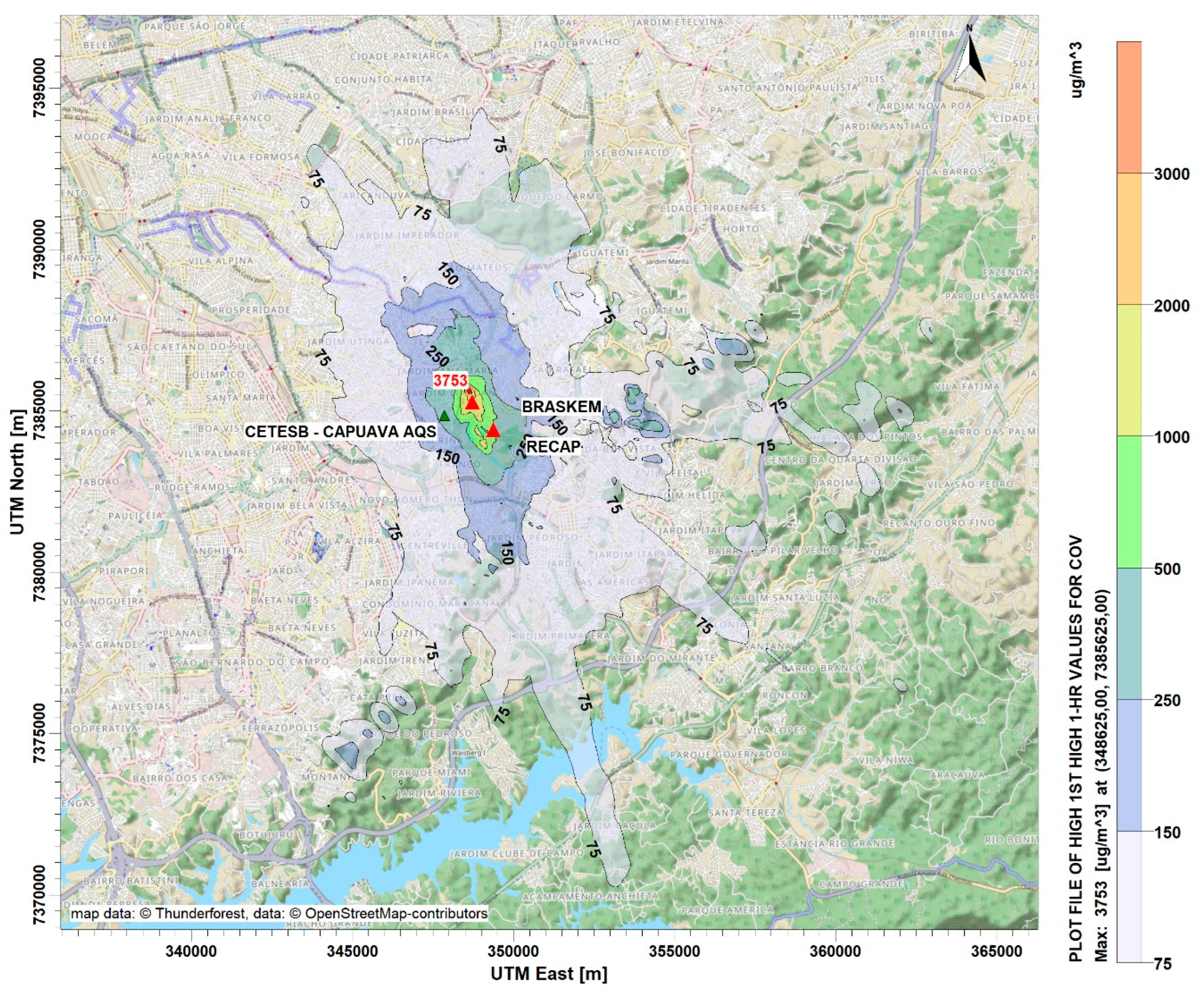
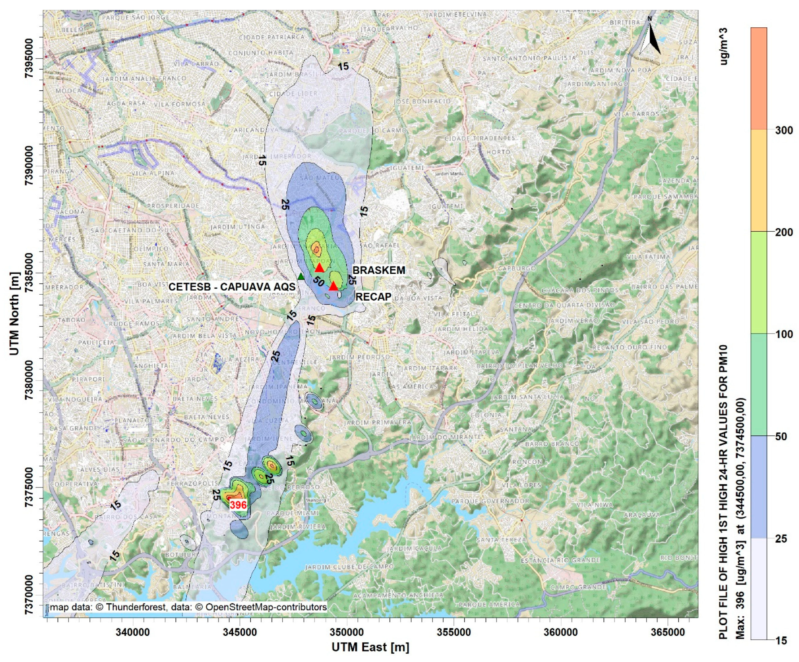
3.2. Air Quality Modeling

The AERMOD model gives a 1 h average for PM and VOC concentrations providing temporal series that were compared with the data of benzene, toluene, and PM10 from Capuava AQS (Figure 6a). For this purpose, the data were filtered by the wind direction, considering only hourly data when the wind direction was in the preferred quadrant for CPC emissions (0–180°) (Figure 6b). The comparison between PM and VOC provided by AERMOD and PM10, benzene, and toluene was provided. In general, the minimum and maximum values coincided with the AERMOD data versus the Capuava AQS data. These results also indicate that the AQS is well located and has a significant representative area.
Positive correlations were observed between VOC–AERMOD and benzene-AQS (r = 0.62), and for VOC–AERMOD and toluene-AQS (r = 0.26). A linear correlation indicates that CPC could be responsible for more than 60% of benzene behavior in the Capuava AQS. Considering all of the limitations of the Gaussian plume model in a complex urban atmosphere, this is a satisfactory result (Figure 6a), although toluene showed poor levels of linear correlation (r = 0.26).
The linear correlation between benzene and toluene measurements from the Capuava AQS was less than 50% (r = 0.49). From the observations of the diurnal profile (Figure 4), we can consider that pollutants were emitted by the same sources, as discussed earlier. However, a possible explanation for the low correlation between them is that toluene emissions were more intense than for benzene. These findings, along with our observations here, lead us to some possible explanations, such as that the emission of benzene was not as constant as that of toluene. Benzene emissions can result either from a less-used product or from the activation of a sporadic production line, resulting in fewer emissions.
The low level of the PM linear correlation that followed (PM–AERMOD and PM10-AQS (r = 0.33)) was an unexpected result. The simulation conditions (industrial sources, near-field model, very close weather station, and good description of building downwash) were appropriate for modeling a pollutant such as PM10. This poorer result of linear correlation (r = 0.33) makes it evident that local traffic has an important role in the emissions of particulate matter. However, vehicle and truck traffic could not explain the behavior of early morning peaks, or the soot layers observed on the houses. Therefore, it is quite possible that the emissions inventory used in the EIA is incomplete or underestimated.
In operational conditions, PM emission rates around 2 g s−1 are acceptable; however, in poor burning conditions, this value may be an order of magnitude higher [59,60]. Flaring is the common practice of burning unwanted, flammable gases via combustion in an open atmosphere, usually to avoid system overload. Although flares are a security system to prevent explosions and to ensure the operational integrity of the refinery [61], using them is not an effective emission control system as a combustion chamber [61]. The frequent use of the flare can be interpreted as an under-dimensioning of the atmospheric emission treatment system (combustion chamber, gas scrubber, etc.), resulting in an unnecessary level of exposure of the surrounding population to PM.
The pollutants’ dispersion provided by AERMOD is shown in Figure 7 and Figure 8. The maximum concentration of the 1 h average of VOC (3.753 µg m−3, 23°37′58.59″ S, 46°29′2.37″ W) is highlighted in Figure 7, during April and May of 2021. It is very important to observe that this highest VOC value modeled by AERMOD happened, practically, inside the CPC area. Therefore, when observing the dispersion of the plume, it could be verified that the residential area was exposed to concentrations that varied from 75 to 500 µg m−3 (areas in different shades of blue in Figure 7). These values are consistent with the event observed by official air quality monitoring [6] and are compatible with the levels of odor perception [62]. The plume of 75 µg m−3 concentration reached areas from 8 to 19 km away from the complex, and the plume ranging from 250 to 1000 µg m−3 reached the nearest areas, about 3 km away.
This aspect of concentration isolines (centered at the source, with low dilution rates) is typical of industries whose fugitive emissions (tanks, valves, and pipes) are predominant. Whenever the odorous substances were emitted from fugitive sources, the plume tended to remain close to the ground (near the urban canopy) with low dilution rates (or high concentration levels) which would explain the fact that closer residents reported large discomfort [7,58]. The VOC result modeling was consistent with the areas where odor reports occurred. However, the simulated concentrations were too low to generate odor discomfort as reported by local people. However, higher concentrations were registered by Capuava AQS, indicating that the odor might have been generated by uncontrolled emissions that were higher than the values established by the environmental licenses. The reports obtained from local people mentioned slightly sweet unpleasant odors, headaches, and nausea, whereby these descriptions are consistent with benzene contamination [9]. While most countries have different and long-term (between 5 and 10 µg m−3 according to annual average) standards for benzene, Brazil does not define the air quality standard for it. The few short-term air quality standards for benzene are as follows: 300 µg m−3 (20-min, Russia); 22 µg m−3 (1 h, Vietnam); 5 µg m−3 (8 h, Albania); and 3.9 µg m−3 (24 h, Israel) [9]. Comparing 1 h Capuava AQS data (Figure 3 and Figure 4) with the Vietnam air quality standard (22 µg m−3, 1 h) [9], some exceedances of the air quality standard could be observed during the April/May 2021 episode, which did not occur in the previous years, evidencing possible higher uncontrolled emissions of VOC.
The PM isolines showed the 396 µg m−3 maximum 24 h average concentration, (23°43′26.30″ S, 46°31′31.37″ W) which occurred 10 km southwest from CPC (Figure 8). The plume ranging from 100 to 200 µg m−3, with second maximum concentration of the 300 µg m−3, reached areas closer to the sources, about 2 km away.
These extended distances of PM happened when the releases from the source had enough energy to reach the higher parts of the boundary layer and carried out the advection process more intensively. The CPC flare launched the PM from 110 m high and at temperatures above 1000 °C. These conditions allowed the pollutants to reach the top of the boundary layer effortlessly, keeping the pollutants in suspension for a longer time, suffering slow dry depletion and resulting in layers of soot on the houses, as noted by several residents [7,58]. The secondary maximum area occurrence (≥200 and ≤350 µg m3) was the outcome of the building downwash effect in low wind and stable atmosphere (or a low height of the boundary layer). This result may have indicated that CPC emissions produced high PM concentrations in the vicinity, which to a certain extent can explain the early morning peaks observed in the Capuava AQS (Figure 5).

4. Conclusions

CPC carried out a 50-day scheduled shutdown for the maintenance, resulting in severe uncontrolled emissions of PM and VOCs in a densely populated and residential area (~3400 inhabitants/km2). The absence of information about the release of odorous gas and soot into the atmosphere makes it impossible to carry out more accurate analyses. However, by using existing AQS data and the dispersion model, it was possible to estimate the impact on the air quality from these emissions in MASP, especially in the ABC region.
The episode period of uncontrolled emissions (April–May 2021) was statistically analyzed by comparing the previous (2017–2020) and the subsequent (2021–2022) periods. When we compared annual 1 h concentrations and the diurnal profiles from the four previous years, an increase in the mean concentrations was observed by a factor of 2 for PM10, benzene, and toluene, reaching maximum values during the episode: 174 µg m−3 (PM10), 79.1 µg m−3 (benzene), and 58.7 µg m−3 (toluene). The description of the odor and symptoms presented by the local population, in the same period, were compatible with the presence of benzene and other volatile substances. The reports of soot deposition in the houses can be explained by PM10 which showed unexpected peaks that could not be associated with special meteorological events or typical profiles of traffic emissions in that area. These reports by the population were compatible with the Braskem and RECAP public declarations about the more intense use of the flare before and after the maintenance period.
Meanwhile, these higher concentrations continued to be observed after the episode, but their variation cannot be fully explained yet. However, it is worth highlighting that this corresponds to the post-pandemic period and the 2022 data also correspond to the period from January to June, that is, they do not represent the annual variation.
Additionally, the estimation by the AERMOD model showed that the VOC plume could potentially reach a large part of the Mauá and Santo André municipalities and the east side of São Paulo city. A linear correlation indicated that CPC could be responsible for more than 60% of benzene concentrations in the Capuava AQS. In this case, we could consider the Capuava AQS to be well-positioned regarding these pollutants’ concentrations, resulting from CPC emissions with good spatial representation for this type of source, with most of them being fugitives and near-canopy advection.
The maximum concentration of PM was observed far from the CPC area (~10 km) in São Bernardo do Campo municipality, increasing the amount of people exposed to these emissions, which can explain the poor correlation between modeled versus AQS data (r = 0.33). In this way, AQS probably cannot perform accurate PM measurements or they are being underestimated, considering the height of the sources (stacks and flares), presenting a plume that reaches a larger area. Additionally, it is quite possible that the emissions inventory used in the EIA is incomplete or underestimated. However, the several reports of soot on houses in the neighborhoods close to the CPC, associated with the turned-on flares and early morning peaks of PM10 in Capuava AQS, indicate the local impact of these industrial activities.
Many studies around the world are aiming to evaluate some industrial source types and current discussions about their effects on air quality have been developed in different places [63,64,65,66,67]. However, in Brazil, few studies address this topic as little is known about the emissions inventory, VOC speciation, or PM chemical composition for industrial emissions [2,33,34,68,69]. To conclude, our results provide significantly important information on the effects of airborne emissions from the CPC on air quality in a densely urbanized area, analyzing data from an official AQS and modeled results (AERMOD) for a special episode of air contamination in Brazil.

Supplementary Materials

The following supporting information can be downloaded at https://www.mdpi.com/article/10.3390/atmos14030577/s1: Table S1: Summary of statistical analysis for hourly concentrations (µg m−3) in the Capuava AQS during 2017 to 2022, and modeled data provided by AERMOD; Table S2: Summary of AERMOD input data extracted from environmental licenses of Braskem and RECAP; Table S3: Summary of statistical analysis of AERMET input data; Figure S1: Changes in benzene, toluene, and PM10 mean hourly concentrations at Capuava station, depending on wind directions. (a) Polar annulus plots from 2017 to 2020 and (b) polar annulus plots for episode from April to May 2021. Color scale represents concentrations (µg m−3), and the thickness in the circle represents the hour of the day: 00:00 inside to 11:00 p.m. outside. Empty spaces are missing values.

Author Contributions

M.S.C. and D.C.Z. conducted the analysis of the data and the conceptualization of the present study. D.C.Z. and T.S.d.P. performed the model analysis. M.S.C. wrote the paper. D.C.Z., A.F., and R.Y.Y. assisted with the data interpretation and the review of the manuscript drafts. All authors have read and agreed to the published version of the manuscript.

Funding

This research is funded by FAPESP (2020/07141-2).

Institutional Review Board Statement

Not applicable.

Informed Consent Statement

Not Applicable.

Data Availability Statement

The data are available upon request.

Acknowledgments

The authors thank FAPESP (2020/07141-2) and CNRS-France for the founding of the international collaboration project (BIOMASP+). The authors thank the financial support and scholarship (Monique Silva Coelho) of CAPES-PROEX (post-graduate program in Meteorology, IAG-USP).

Conflicts of Interest

The authors declare that they have no known competing financial interests or personal relationships that could have appeared to influence the work reported in this paper.

Abbreviations

PhraseAcronym
Metropolitan area of São PauloMASP
Capuava Petrochemical ComplexCPC
Capuava Oil RefineryRECAP
Air quality stationAQS
Environmental Agency of São Paulo StateCETESB
Environmental impact assessments EIA
Steady-state plume modelAERMOD
California Puff: non-steady-state puff dispersion modelCALPUFF
Flexible particle dispersion modelFLEXPART
Community multiscale air qualityCMAQ
Hybrid single-particle Lagrangian integrated trajectoryHYSPLIT
Stable boundary layerSBL
Convective boundary layerCBL
Benzene, toluene, ethylbenzene, and xylenesBTEX

References

  1. CETESB Multa Empresas Do Polo Petroquímico Capuava. Available online: https://cetesb.sp.gov.br/blog/2021/04/14/cetesb-multa-empresas-do-polo-petroquimico-capuava/ (accessed on 10 June 2021).
  2. Coelho, M.S.; Dominutti, P.A.; Boian, C.; dos Santos, T.C.; Nogueira, T.; Oliveira, C.A.V.B.d.S.; Fornaro, A. Non-methane hydrocarbons in the vicinity of a petrochemical complex in the Metropolitan Area of São Paulo, Brazil. Air Qual. Atmos. Health 2021, 14, 967–984. [Google Scholar] [CrossRef]
  3. Evo, C.P.R.; Ulrych, B.K.; Takegawa, B.; Soares, G.; Nogueira, G.; Oliveira, L.O.D.; Golfetti, M.; Milazzotto, P.H.; Martins, L.C. Poluição Do Ar e Internação Por Insuficiência Cardíaca Congestiva Em Idosos No Município de Santo André Air Pollution and Congestive Heart Failure Hospital Admissions on Elderly in Santo André. Arq. Bras. Ciência da Saúde 2011, 36, 6–9. [Google Scholar]
  4. Saiki, M.; Alves, E.R.; Marcelli, M.P. Analysis of lichen species for atmospheric pollution biomonitoring in the Santo André Municipality, São Paulo, Brazil. J. Radioanal. Nucl. Chem. 2007, 273, 543–547. [Google Scholar] [CrossRef]
  5. Petrobras Refinaria Capuava. Available online: https://petrobras.com.br/pt/nossas-atividades/principais-operacoes/refinarias/refinaria-capuava-recap.htm (accessed on 10 March 2020).
  6. CETESB. Qualidade Do Ar No Estado de São Paulo. 2022; p. 228. Available online: http://cetesb.sp.gov.br/ar/piblicacoes-relatorios/ (accessed on 28 February 2022).
  7. ABC, D.d.G. Forte Cheiro de Queimado Preocupa Moradores Da Região. Available online: https://www.dgabc.com.br/Noticia/3705274/forte-cheiro-de-queimado-preocupa-moradores-da-regiao (accessed on 9 April 2021).
  8. Otto, D.; Molhave, L.; Rose, G.; Hudnell, H.K.; House, D. Neurobehavioral and sensory irritant effects of controlled exposure to a complex mixture of volatile organic compounds. Neurotoxicol. Teratol. 1990, 12, 649–652. [Google Scholar] [CrossRef] [PubMed]
  9. Sekar, A.; Varghese, G.K.; Ravi Varma, M.K. Analysis of benzene air quality standards, monitoring methods and concentrations in indoor and outdoor environment. Heliyon 2019, 5, e02918. [Google Scholar] [CrossRef] [PubMed] [Green Version]
  10. Dominutti, P.; Nogueira, T.; Fornaro, A.; Borbon, A. One Decade of VOCs Measurements in São Paulo megacity: Composition, variability, and emission evaluation in a biofuel usage context. Sci. Total Environ. 2020, 738, 139790. [Google Scholar] [CrossRef]
  11. Zhang, Q.; Sun, L.; Wei, N.; Wu, L.; Mao, H. The characteristics and source analysis of VOCS emissions at roadside: Assess the impact of ethanol-gasoline implementation. Atmos. Environ. 2021, 263, 118670. [Google Scholar] [CrossRef]
  12. Mao, W.; Wang, W.; Jiao, L.; Zhao, S.; Liu, A. Modeling air quality prediction using a deep learning approach: Method optimization and evaluation. Sustain. Cities Soc. 2021, 65, 102567. [Google Scholar] [CrossRef]
  13. Liu, Y.; Wang, H.; Jing, S.; Peng, Y.; Gao, Y.; Yan, R.; Wang, Q.; Lou, S.; Cheng, T.; Huang, C. Strong regional transport of volatile organic compounds (VOCs) during wintertime in Shanghai megacity of China. Atmos. Environ. 2021, 244, 117940. [Google Scholar] [CrossRef]
  14. Xu, H.; Li, Y.; Feng, R.; He, K.; Ho, S.S.H.; Wang, Z.; Ho, K.F.; Sun, J.; Chen, J.; Wang, Y.; et al. Comprehensive characterization and health assessment of occupational exposures to volatile organic compounds (VOCs) in Xi’an, a major city of Northwestern China. Atmos. Environ. 2021, 246, 118085. [Google Scholar] [CrossRef]
  15. Harrison, R.M.; Allan, J.; Carruthers, D.; Heal, M.R.; Lewis, A.C.; Marner, B.; Murrells, T.; Williams, A. Non-exhaust vehicle emissions of particulate matter and voc from road traffic: A review. Atmos. Environ. 2021, 262, 118592. [Google Scholar] [CrossRef]
  16. Gao, Y.; Li, M.; Wan, X.; Zhao, X.; Wu, Y.; Liu, X.; Li, X. Important contributions of alkenes and aromatics to VOCs emissions, chemistry and secondary pollutants formation at an industrial site of central Eastern China. Atmos. Environ. 2021, 244, 117927. [Google Scholar] [CrossRef]
  17. Andrade, M.F.; Kumar, P.; Freitas, E.D.; Ynoue, R.Y.; Martins, J.; Martins, L.D.; Nogueira, T.; Perez-Martinez, P.; Miranda, R.M.; Albuquerque, T.; et al. Air quality in the megacity of São Paulo: Evolution over the last 30 years and future perspectives. Atmos. Environ. 2017, 159, 66–82. [Google Scholar] [CrossRef] [Green Version]
  18. Bali, K.; Kumar, A.; Chourasiya, S. Emission estimates of trace gases (VOCs and NOx) and their reactivity during biomass burning period (2003–2017) over Northeast India. J. Atmos. Chem. 2021, 78, 17–34. [Google Scholar] [CrossRef]
  19. World Health Organization. Air Quality Guidelines: Particulate Matter (PM2.5 and PM10), Ozone, Nitrogen Dioxide, Sulfur Dioxide and Carbon Monoxide. 2021. Available online: https://apps.who.int/iris/handle/10665/345329 (accessed on 20 November 2022).
  20. Lee, S.C.; Chiu, M.Y.; Ho, K.F.; Zou, S.C.; Wang, X. Volatile organic compounds (VOCs) in Urban atmosphere of Hong Kong. Chemosphere 2002, 48, 375–382. [Google Scholar] [CrossRef] [PubMed]
  21. Tiwari, V.; Hanai, Y.; Masunaga, S. Ambient levels of volatile organic compounds in the vicinity of petrochemical industrial area of Yokohama, Japan. Air Qual. Atmos. Health 2010, 3, 65–75. [Google Scholar] [CrossRef] [Green Version]
  22. Leuchner, M.; Rappenglück, B. VOC Source-receptor relationships in Houston during TexAQS-II. Atmos. Environ. 2010, 44, 4056–4067. [Google Scholar] [CrossRef]
  23. Sergio Chiarelli, P.; Amador Pereira, L.A.; Nascimento Saldiva, P.H.d.; Ferreira Filho, C.; Bueno Garcia, M.L.; Ferreira Braga, A.L.; Conceição Martins, L. The association between air pollution and blood pressure in traffic controllers in Santo Andre, São Paulo, Brazil. Environ. Res. 2011, 111, 650–655. [Google Scholar] [CrossRef]
  24. Zaccarelli-Marino, M.A. Chronic autoimmune thyroiditis in industrial areas in Brazil: A 15-year survey. J. Clin. Immunol. 2012, 32, 1012–1018. [Google Scholar] [CrossRef]
  25. Zaccarelli-Marino, M.A.; André, C.D.S.; Singer, J.M. Overt primary hypothyroidism in an industrial area in São Paulo, Brazil: The impact of public disclosure. Int. J. Environ. Res. Public Health 2016, 13, 1161. [Google Scholar] [CrossRef] [Green Version]
  26. Zaccarelli-Marino, M.A.; Alessi, R.; Balderi, T.Z.; Martins, M.A.G. Association between the occurrence of primary hypothyroidism and the exposure of the population near to industrial pollutants in São Paulo State, Brazil. Int. J. Environ. Res. Public Health 2019, 16, 3464. [Google Scholar] [CrossRef] [PubMed] [Green Version]
  27. United States Environmental Protection Agency. Air Quality Dispersion Modeling—Preferred and Recommended Models. Available online: https://www.epa.gov/scram/air-quality-dispersion-modeling-preferred-and-recommended-models#aermod (accessed on 9 August 2022).
  28. United States Environmental Protection Agency. Air Quality Dispersion Modeling—Alternative Models. Available online: https://www.epa.gov/scram/air-quality-dispersion-modeling-alternative-models#calpuff (accessed on 28 September 2022).
  29. Pisso, I.; Sollum, E.; Grythe, H.; Kristiansen, N.I.; Cassiani, M.; Eckhardt, S.; Arnold, D.; Morton, D.; Thompson, R.L.; Groot Zwaaftink, C.D.; et al. The lagrangian particle dispersion model FLEXPART version 10.4. Geosci. Model Dev. 2019, 12, 4955–4997. [Google Scholar] [CrossRef] [Green Version]
  30. United States Environmental Protection Agency. CMAQ: Community Multiscale Air Quality Modeling System. Available online: https://www.epa.gov/cmaq/frequent-cmaq-questions (accessed on 25 October 2022).
  31. Bihałowicz, J.S.; Rogula-Kozłowska, W.; Krasuski, A. Contribution of landfill fires to air pollution—An assessment methodology. Waste Manag. 2021, 125, 182–191. [Google Scholar] [CrossRef]
  32. Venkatram, A.; Brode, R.; Cimorelli, A.; Lee, R.; Paine, R.; Perry, S.; Peters, W.; Weil, J.; Wilson, R. A complex terrain dispersion model for regulatory applications. Atmos. Environ. 2001, 35, 4211–4221. [Google Scholar] [CrossRef]
  33. Cerqueira, J.S.; de Albuquerque, H.N.; Sousa, F.A.S. Atmospheric pollutants: Modeling with Aermod software. Air Qual. Atmos. Health 2018, 12, 21–32. [Google Scholar] [CrossRef]
  34. Macêdo, M.F.M.; Ramos, A.L.D. Vehicle atmospheric pollution evaluation using AERMOD. Model at avenue in a Brazilian capital city. Air Qual. Atmos. Health 2020, 13, 309–320. [Google Scholar] [CrossRef]
  35. Kelleghan, D.B.; Hayes, E.T.; Everard, M.; Curran, T.P. Predicting atmospheric ammonia dispersion and potential ecological effects using monitored emission rates from an intensive laying hen facility in Ireland. Atmos. Environ. 2021, 247, 118214. [Google Scholar] [CrossRef]
  36. Pirhalla, M.; Heist, D.; Perry, S.; Tang, W.; Brouwer, L. Simulations of dispersion through an irregular urban building array. Atmos. Environ. 2021, 258, 118500. [Google Scholar] [CrossRef]
  37. Tyovenda, A.A.; Ayua, T.J.; Sombo, T. Modeling of gaseous pollutants (CO and NO2) emission from an industrial stack in Kano City, Northwestern Nigeria. Atmos. Environ. 2021, 253, 118356. [Google Scholar] [CrossRef]
  38. Pecha, P.; Tichý, O.; Pechová, E. Determination of radiological background fields designated for inverse modelling during atypical low wind speed meteorological episode. Atmos. Environ. 2021, 246, 118105. [Google Scholar] [CrossRef]
  39. Cimorelli, A.J.; Perry, S.G.; Venkatram, A.; Weil, J.C.; Paine, R.B.; Wilson, R.B.; Russell, R.L.; Peters, W.D.; Brode, R.W. AERMOD: A dispersion model for industrial source applications. part I: General model formulation and boundary layer characterization. J. Appl. Meteorol. Climatol. 2005, 44, 682–693. [Google Scholar] [CrossRef]
  40. Motalebi Damuchali, A.; Guo, H. Developing an odour emission factor for an oil refinery plant using reverse dispersion modeling. Atmos. Environ. 2020, 222, 117167. [Google Scholar] [CrossRef]
  41. Hennig, T.A.; Kretsch, J.L.; Pessagno, C.J.; Salamonowicz, P.H.; Stein, W.L. The shuttle radar topography mission. In Digital Earth Moving. Lecture Notes in Computer Science; Westort, C.Y., Ed.; Springer: Berlin/Heidelberg, Germany, 2001; Volume 2181, pp. 65–77. [Google Scholar] [CrossRef]
  42. Carslaw, D.C.; Ropkins, K. Openair—An r package for air quality data analysis. Environ. Model. Softw. 2012, 27–28, 52–61. [Google Scholar] [CrossRef]
  43. Cui, Y.; Ji, D.; He, J.; Kong, S.; Wang, Y. In situ continuous observation of hourly elements in PM2.5 in urban Beijing, China: Occurrence levels, temporal variation, potential source regions and health risks. Atmos. Environ. 2020, 222, 117164. [Google Scholar] [CrossRef]
  44. Kamara, A.A.; Harrison, R.M. Analysis of the air pollution climate of a central urban roadside supersite: London, marylebone road. Atmos. Environ. 2021, 258, 118479. [Google Scholar] [CrossRef]
  45. Squizzato, R.; Nogueira, T.; Martins, L.D.; Martins, J.A.; Astolfo, R.; Machado, C.B.; Andrade, M.d.F.; Freitas, E.D.d. Beyond megacities: Tracking air pollution from urban areas and biomass burning in Brazil. Clim. Atmos. Sci. 2021, 4, s41612–s41621. [Google Scholar] [CrossRef]
  46. Vestenius, M.; Hopke, P.K.; Lehtipalo, K.; Petäjä, T.; Hakola, H.; Hellén, H. Assessing volatile organic compound sources in a boreal forest using positive matrix factorization (PMF). Atmos. Environ. 2021, 259, 118503. [Google Scholar] [CrossRef]
  47. Dominutti, P.A.; Nogueira, T.; Borbon, A.; Andrade, M.d.F.; Fornaro, A. One-year of NMHCs hourly observations in São Paulo Megacity: Meteorological and traffic emissions effects in a large ethanol burning context. Atmos. Environ. 2016, 142, 371–382. [Google Scholar] [CrossRef]
  48. Chang, J.C.; Hanna, S.R. Air quality model performance evaluation. Meteorol. Atmos. Phys. 2004, 87, 167–196. [Google Scholar] [CrossRef]
  49. Parrish, D.D.; Trainer, M.; Young, V.; Goldan, P.D.; Kuster, W.C.; Jobson, B.T.; Fehsenfeld, F.C.; Lonneman, W.A.; Zika, R.D.; Farmer, C.T.; et al. Internal consistency tests for evaluation of measurements of anthropogenic hydrocarbons in the troposphere. J. Geophys. Res. 1998, 103, 339–359. [Google Scholar] [CrossRef]
  50. Carvalho, V.S.B.; Freitas, E.D.; Martins, L.D.; Martins, J.A.; Mazzoli, C.R.; Andrade, M.d.F. Air quality status and trends over the metropolitan area of São Paulo, Brazil as a result of emission control policies. Environ. Sci. Policy 2015, 47, 68–79. [Google Scholar] [CrossRef]
  51. Valverde, M.C.; Coelho, L.H.; de Oliveira Cardoso, A.; Paiva Junior, H.; Brambila, R.; Boian, C.; Martinelli, P.C.; Valdambrini, N.M. Urban climate assessment in the ABC Paulista Region of São Paulo, Brazil. Sci. Total Environ. 2020, 735, 139303. [Google Scholar] [CrossRef] [PubMed]
  52. Jiang, Z.; Grosselin, B.; Daële, V.; Mellouki, A.; Mu, Y. Seasonal and diurnal variations of BTEX compounds in the semi-urban environment of Orleans, France. Sci. Total Environ. 2017, 574, 1659–1664. [Google Scholar] [CrossRef] [PubMed]
  53. Simpson, I.J.; Blake, N.J.; Barletta, B.; Diskin, G.S.; Fuelberg, H.E.; Gorham, K.; Huey, L.G.; Meinardi, S.; Rowland, F.S.; Vay, S.A.; et al. Characterization of trace gases measured over alberta oil sands mining operations: 76 speciated C2-C10 volatile organic compounds (VOCs), CO2, CH4, CO, NO, NO2, NOy, O3 and SO2. Atmos. Chem. Phys. 2010, 10, 11931–11954. [Google Scholar] [CrossRef] [Green Version]
  54. Ragothaman, A.; Anderson, W.A. Air quality impacts of petroleum refining and petrochemical industries. Environment 2017, 4, 66. [Google Scholar] [CrossRef] [Green Version]
  55. Atkinson, R.; Arey, J. Atmospheric degradation of volatile organic compounds atmospheric degradation of volatile organic compounds. Chem. Rev. 2003, 103, 4605–4638. [Google Scholar] [CrossRef]
  56. Braskem. Busca de Produtos. Available online: http://www.braskem.com/busca-de-produtos (accessed on 13 August 2020).
  57. ABC DO ABC. Available online: https://www.abcdoabc.com.br/abc/noticia/atuacao-braskem-polo-petroquimico-grande-abc-50400 (accessed on 14 August 2020).
  58. ABC, D.d.G. Moradores Vizinhos Relatam Aumento Da Poluição Do Ar. Available online: https://www.dgabc.com.br/Noticia/3679176/moradores-vizinhos-relatam-aumento-da-poluicao-do-ar (accessed on 16 February 2021).
  59. Johnson, M.R.; Devillers, R.W.; Thomson, K.A. Quantitative field measurement of soot emission from a large gas flare using sky-LOSA. Environ. Sci. Technol. 2011, 45, 345–350. [Google Scholar] [CrossRef] [Green Version]
  60. McEwen, J.D.N.; Johnson, M.R. Black carbon particulate matter emission factors for buoyancy-driven associated gas flares. J. Air Waste Manag. Assoc. 2012, 62, 307–321. [Google Scholar] [CrossRef] [Green Version]
  61. CETESB. Poluição Do Ar: Gerenciamento e Controle de Fontes. Conform. Ambient. Com Requisitos Técnicos E Legais 2017, 2, 254. [Google Scholar]
  62. Gutiérrez, M.C.; Hernández-Ceballos, M.A.; Márquez, P.; Chica, A.F.; Martín, M.A. Identification and simulation of atmospheric dispersion patterns of odour and VOCs generated by a waste treatment plant. Atmos. Pollut. Res. 2023, 14, 101636. [Google Scholar] [CrossRef]
  63. Lin, Y.C.; Lai, C.Y.; Chu, C.P. Air Pollution diffusion simulation and seasonal spatial risk analysis for industrial areas. Environ. Res. 2021, 194, 110693. [Google Scholar] [CrossRef] [PubMed]
  64. Parveen, N.; Siddiqui, L.; Sarif, N.; Islam, S.; Khanam, N.; Mohibul, S. Industries in Delhi: Air pollution versus respiratory morbidities. Process. Saf. Environ. Prot. 2021, 152, 495–512. [Google Scholar] [CrossRef]
  65. Arulprakasajothi, M.; Chandrasekhar, U.; Yuvarajan, D.; Teja, M.B. An analysis of the implications of air pollutants in Chennai. Int. J. Ambient. Energy 2020, 41, 209–213. [Google Scholar] [CrossRef]
  66. Bergstra, A.D.; Brunekreef, B.; Burdorf, A. The Influence of Industry-Related Air Pollution on Birth Outcomes in an Industrialized Area. Environ. Pollut. 2021, 269, 115741. [Google Scholar] [CrossRef] [PubMed]
  67. Michalik, J.; Machaczka, O.; Jirik, V.; Heryan, T.; Janout, V. Air pollutants over industrial and non-industrial areas: Historical concentration estimates. Atmosphere 2022, 13, 455. [Google Scholar] [CrossRef]
  68. Tadano, Y.S.; Mazza, R.A.; Tomaz, E. Modelagem Da Dispersão De Poluentes Atmosféricos No Município De Paulínia (Brasil) Empregando O Iscst3. Mecánica Comput. 2010, XXIX, 8125–8148. [Google Scholar]
  69. Kawashima, A.B.; Martins, L.D.; Rafee, S.A.A.; Rudke, A.P.; de Morais, M.V.; Martins, J.A. Development of a spatialized atmospheric emission inventory for the main industrial sources in Brazil. Environ. Sci. Pollut. Res. 2020, 27, 35941–35951. [Google Scholar] [CrossRef]
Figure 1. Metropolitan area of São Paulo (MASP) with Braskem and RECAP industries, and the CETESB, Capuava Air Quality Station, and AQS (identified by the red triangles). Source: OpenStreetMap.
Atmosphere 14 00577 g001
Figure 2. Braskem and RECAP industrial plants on tridimensional modeling. In blue are the buildings or tanks, in red are the point sources (stacks/flare). Source: Google Earth (accessed on 11 March 2023).
Atmosphere 14 00577 g002
Figure 3. Annual boxplots of 1 h concentrations (µg m−3) for PM10, benzene, and toluene at Capuava AQS, from 2017 to 2022, and for each episode. Boxplot width and the lower and upper hinges correspond to the first and third quartiles (the 25th and 75th percentiles). Lower whisker: smallest observation greater than or equal to lower hinge—1.5 * IQR (interquartile range), above 75th percentile. Upper whisker: largest observation less than or equal to upper hinge + 1.5 * IQR, below 25th percentile. The middle is the median (50% quantile), and the red point is the mean value. Points beyond the end of the whiskers are “outliers”, which correspond to values > 1.5 and <3 times the standard deviation (sd). The data were presented on the Y axis with an appropriate scale for good visualization of the percentiles and the mean in relation to the median. Obs.: The episode corresponds to April–May of 2021, 2021 corresponds to the other months of this year, the data available for 2020 were only from January to March, and 2022 was only from January to June.
Atmosphere 14 00577 g003
Figure 4. Normalized concentrations in relation to the mean value profiles for PM10, benzene, and toluene at Capuava AQS, from April to May for each year from 2017 to 2022. Episode represents the 2021 concentrations.
Atmosphere 14 00577 g004
Figure 5. Hourly concentrations of PM10 at Capuava AQS, during the episode (April to May 2021). Rectangles represent the peaks observed from 1:00 a.m. to 4:00 a.m.
Atmosphere 14 00577 g005
Figure 6. (a) Hourly mean concentrations for benzene, toluene, and PM10 at Capuava AQS, VOC, and PM (AERMOD: modeled data) during the episode (April to May 2021), white spaces are missing values. (b) The wind rose shows the wind speed (m s−1) and wind direction (°), data were filtered by the preferential wind direction from the Capuava Petrochemical Complex (0° to 180°) (c) “Correlation” is the correlation coefficient of Pearson.
Atmosphere 14 00577 g006
Figure 7. The maximum concentration of 1 h average (µg m−3) of VOC in the affected area during the CPC maintenance period.
Atmosphere 14 00577 g007
Figure 8. The maximum concentration of 24 h average (µg m−3) of PM in the affected area during the CPC maintenance period.
Atmosphere 14 00577 g008
Disclaimer/Publisher’s Note: The statements, opinions and data contained in all publications are solely those of the individual author(s) and contributor(s) and not of MDPI and/or the editor(s). MDPI and/or the editor(s) disclaim responsibility for any injury to people or property resulting from any ideas, methods, instructions or products referred to in the content.

