Article

Research on Temporal and Spatial Distribution of Carbon Emissions from Urban Buses Based on Big Data Analysis

School of Modern Post, Xi’an University of Posts & Telecommunications, Xi’an 710061, China
*
Author to whom correspondence should be addressed.
Atmosphere 2023, 14(2), 411; https://doi.org/10.3390/atmos14020411
Submission received: 19 December 2022 / Revised: 3 February 2023 / Accepted: 15 February 2023 / Published: 20 February 2023
(This article belongs to the Special Issue Road Transportation Carbon Emissions and Decarbonization Pathways)

Abstract

:
In recent years, global warming has become increasingly severe, and the ecological and environmental problems facing mankind have become increasingly serious. As the main areas of transportation activities, cities are also the main places of carbon emissions. As a necessary condition for human’s daily-life travel, it is particularly important to calculate the carbon emissions from urban transportation. Due to the different characteristics of economy and population in different regions of a city, the carbon emissions of urban buses show different characteristics in terms of temporal and spatial distribution. The developments of science and technology promote the application of big data analysis to specific practical life, enabling people to research and solve problems from a new perspective. This paper uses the GPS data of urban buses in Sanya City, China, to identify operation conditions from urban buses, and calculates the distance and time under different conditions. Based on the measured data of carbon emissions, this paper visualizes the distribution characteristics of carbon emissions by density analysis; explains the time distribution characteristics by the visual analysis of carbon emissions in different time periods, working days and rest days, and different energy types; and illustrates the spatial distribution characteristics by the spatial distributions of carbon emissions from Sanya’s buses on working days and rest days, as well as in different routes, providing reference for a low-carbon development of urban green transport.

1. Introduction

In the process of urbanization, the urban population is increasing day by day. Urban public transport (such as buses, subways, and taxis) has become an increasingly important travel mode advocated by the government and urban residents because of its low carbon, efficient, and convenient characteristics [1]. Compared with other urban transportation tools, such as subway, taxi, and private car, urban buses have the advantages of low cost, wide distribution of line stations, short distance between stations, high traffic efficiency, and low energy consumption per capita. As an important part of the transportation system, urban buses are an important part of the low-carbon development of urban transportation [2]. In order to control motor vehicle exhaust pollution, China issued the national standard for motor vehicle emissions, “Limits and Measurement Methods of Pollutants from Heavy Diesel Vehicles (China’s Phase VI)” (GB17691-2018), in which the emissions of carbon monoxide (CO) and nitrogen oxides (NOX) should not exceed 500 and 35 mg/km. It has an important practical significance in how to make use of the cutting-edge science and technology and research methods, such as GPS trajectory data, urban point-of-interest data, and big data, to focus on the low-carbon development of urban transportation from multiple perspectives and thus provide data support and theoretical guidance for urban green construction.
At present, research on the carbon emissions of urban transportation at home and abroad includes that on their measurement methods and space–time distributions. In terms of the measurement of the carbon emissions from urban transportation, there are two common computing methods. One is to calculate the carbon emissions based on energy consumption statistics, and the other is to calculate them based on the actual energy consumptions and corresponding carbon emission factors of transportation vehicles in use. So far, there are only relatively few studies on the use of the GPS trajectory data combined with big data mining technology to calculate vehicles’ energy consumptions and carbon emissions.
Sun et al. [3] estimated the carbon emissions of vehicles under different driving modes (such as acceleration, idling, cruising, and deceleration) by using the GPS data to obtain the variables of speed distribution per second. Luo et al. [4] used the GPS data to calculate the average speed of relevant track points, and then obtained the energy consumptions and carbon emissions of taxis. However, the change of driving speed of the whole road network was not considered in the calculation process. In addition, the GPS data only covered 20% of all taxis in Shanghai, so the amount of research data was relatively small. Du et al. [5] used a back-propagation neural network to predict vehicles’ fuel consumptions by the floating data of vehicles and analyzed the difference of the fuel consumption distribution between weekdays and weekends in Beijing’s urban area by comparing heat maps. However, this study only involved the total fuel consumption and did not analyze its changes in a day, nor did it include the carbon emission patterns. Weng et al. [6] carried out the bench test to obtain the GPS trajectory data and fuel consumptions of vehicles, but the big data mining technology was not used, and only one type of vehicle was measured for carbon emissions, which could not reflect the changes in carbon emissions of other types of vehicles and energy-type vehicles in the city. Shan et al. [7] used sparse data to reconstruct vehicle trajectories and input the MOVES model to calculate the energy consumptions and carbon emissions of vehicles. Yi et al. [8] calculated and analyzed the relationship between carbon emissions of buses and taxis after COVID-19 through the use of the GPS data of natural gas buses and taxis, and concluded that when the passenger capacity was reduced by less than 30%, the performance of buses in per capita emissions was still better than that of taxis. However, it is a pity that this study only focused on the vehicle conditions in working days, but data related to weekends and holidays were not collected. Zhou Ye et al. [9] used the GPS data to achieve a dynamic and accurate measurement of the carbon emissions from urban transportation, combined with the data of energy and carbon emission factors, gave a calculation mode for carbon emissions, and calculated the carbon emissions of urban roads. Guo [10] adopted two ideas based on the average speed and the operating condition simulations to collect the results of taxi pollution emissions in Shenzhen by using instruments for testing, and obtained the carbon emission factors under different conditions of road vehicle operations by calculating the results. Niu [11] built a carbon emission model of motor vehicle pollutants in Nanjing City, China, by using the localized key parameters of the big data fusion from transportation. Xu et al. [12] constructed a “speed-energy intensity” model based on the multisource monitoring data in Beijing, and calculated the carbon emissions of vehicles driven by different drivers on the premise of different routes.
In terms of research on the temporal and spatial distribution of carbon emissions, because GPS track data contain information such as time, longitude, and latitude, it provides the possibility for scholars to carry out research on the temporal and spatial distribution of relevant data and the analysis of traffic characteristics, and further promotes the digital and intelligent development of research in the transportation industry. Andrienko G [13] analyzed the GPS data from the perspective of time and space, and analyzed and studied the trend characteristics of traffic trajectory by using a variety of visualization methods. Nam et al. [14] took the GPS travel data of taxis in Seoul as the research object, analyzed and discussed the spatial distribution characteristics of taxi passenger capacity by decomposing the GPS data into units of a uniform size with the grid decomposition, and used geographic weighted regression to model the relationship between density and passenger capacity. The results showed that there was also a certain change in the relationship of passenger flows between motor vehicles and rail transit in different regions. Zhao et al. [15] proposed to use taxi GPS data and urban point-of-interest data to speculate the purpose of residents’ travel, and revealed the spatial–temporal distribution rules and characteristics caused by different travel purposes of residents according to the carbon emission characteristics at different locations during peak periods. Wang [16] analyzed and studied the dynamic traffic environment of Shenzhen City, China, from various aspects, and visually displayed the spatial–temporal accessibility and spatial–temporal distribution attribute characteristics of taxis. Xu [17] studied the temporal and spatial characteristics of residents’ travel activities on working days and rest days based on the GPS data of taxis in Beijing. Wang et al. [18] analyzed the spatial–temporal characteristics of Wuhan City, China, based on its traffic dynamic data and applied the results to practical activities. Zheng et al. [19] visualized the impacts of different factors influencing the spatial and temporal distribution of carbon emissions, showing that the significant spatial agglomeration characteristics of the carbon emissions from urban freight have significant effects, and the spatial agglomeration effects of high-carbon emission areas are more obvious. Ning et al. [20] analyzed the temporal and spatial characteristics and influencing factors of the carbon emissions from the citizens’ travel in Zhengzhou City, China, based on the statistical data.
From the above research, the existing research on the measurement of carbon emissions from urban traffic lacks consideration of energy consumptions from specific models and different fuels, and does not distinguish carbon emissions under different driving conditions in combination with the characteristics of vehicles’ operation. Most of the literature is based on theoretical derivation to build models to carry out calculation and analysis. If an in-depth research is conducted from the perspectives of real-time operational vehicles and the existing problems of the current research, it can obtain more accurate carbon emission values. Among existing spatial–temporal distribution studies, there are many studies on the spatial–temporal characteristics analysis and visualization of the GPS data from urban traffic, but most of them were based on the GPS data of urban taxis to discuss the spatial–temporal characteristics of residents’ travel activities. There is limited literature on the spatial–temporal characteristics analysis of carbon emissions from urban buses. Therefore, this paper will calculate the carbon emissions of the GPS data from urban buses and conduct a spatial–temporal visualization research on their carbon emissions.
In the exhaust emissions of motor vehicles, in addition to CO2, CO, hydrocarbons (HC), nitrogen oxides (NOX), particulate matter (PM), and sulfide (SOX) have also become important factors affecting the ambient air quality of large and medium-sized cities [21]. According to more and more investigations and studies, there is a close relationship between greenhouse gases dominated by CO2 and atmospheric pollutants, and there is an important relationship between atmospheric pollutants and carbon emissions with the same origin and interaction. The prevention and treatment methods between the two also have certain homogeneity [22].
Based on the GPS data of the urban buses’ operation in Sanya, this paper studies the carbon emissions of the urban buses in Sanya. After preprocessing the GPS data of buses in Sanya, according to the operating conditions of different buses, this paper adopts the “distance × energy consumption” method to measure the carbon emissions for the driving process and the “time × energy consumption” method for the idle process. It also makes a visual analysis of the temporal and spatial characteristics of carbon emissions, and explores the temporal and spatial characteristics of carbon emissions and the factors influencing the carbon emissions from urban transport so as to provide a reliable basis for the future development of urban low-carbon transport.

2. Research Methods

2.1. Measurement Method of Carbon Emissions

Carbon emission refers to the process of emissions of greenhouse gases to the outside world in the process of human production and business activities. Greenhouse gases are mainly composed of six gases, including CO2, CH4, and N2O. CO2 emissions account for more than 60% of the total greenhouse gas emissions. Therefore, the carbon emissions in the current study mainly refer to CO2 emissions. For the measurement of carbon emissions, scholars often use the methods proposed by the IPCC; that is, the “top–down” method is used from a macro perspective, and the “bottom–up” method is used from a micro perspective. The “top-down” method is used by Schipper [23] to calculate carbon emissions through the total fuel consumptions and energy inventory guidelines. However, this method cannot discuss the temporal and spatial distribution and specific direction of carbon emissions, and can only calculate the carbon emissions of urban transport from an overall perspective.
The “bottom–up” method is used to calculate the energy consumptions through the vehicle ownership and the mileage data of different types of vehicles, and then calculate the carbon emissions by using the carbon emission factors corresponding to different fuels. The specific equation is as follows:
E = i . j L j × Q i , j × F i
E represents the traffic carbon emissions, and its unit is kg; Qi,j refers to the total consumption of the ith type of fuel and the jth type of traffic mode, and the unit is t; Fi is the carbon emission coefficient of the ith type of fuel, and the unit is kg/t; Lj means the total mileage of the jth type of traffic mode, whose unit is km; i refers to the type of fuel from urban transportation; and j refers to the type of traffic mode.
The “bottom–up” method calculates based on the energy consumptions and the carbon emission factors. The carbon emission factors are generally related to fuel types, and it is impossible to accurately calculate the vehicles’ carbon emissions under different driving conditions. Therefore, it is necessary to establish a carbon emission model based on vehicle working conditions with the help of big data.

2.2. Carbon Emission Model of Motor Vehicles

In order to calculate the carbon emissions of vehicles more accurately, scholars at home and abroad have conducted research on the operational characteristics of vehicles and proposed a calculation model of carbon emissions related to the driving characteristics of vehicles. The model mainly combined the data of exhaust emissions’ characteristic with the driving characteristics of vehicles (such as speed, acceleration, and specific power) to calculate energy consumptions and carbon emissions under different driving characteristics.
Generally, there are two types of emission models for vehicles:
  • Emission model based on average speed
Sun et al. [24] revealed through research that different driving characteristics of vehicles also have different influences on carbon emissions, among which speed has a more significant influence on carbon emissions. Common carbon emission models based on the average speed of vehicles include MOBILE, COPERT, MOVES, and so on. Mainly based on the average speed of motor vehicles during driving, they correct the carbon emission factors and then obtain the total carbon emissions combining the mileage. The specific equation is:
E = L × e v
E represents the traffic carbon emissions, whose unit is kg; L is the total mileage, whose unit is km; and e(v) refers to the carbon emission factor corrected for the average speed, whose unit is kg/km.
2.
Emission model based on driving conditions
The emission model based on driving conditions means that the carbon emissions of vehicles are calculated according to the parameters of instantaneous speed, acceleration, and so on under the running state of the vehicles, which can accurately reflect the instantaneous emissions of the vehicles in seconds under different driving conditions. However, the model needs to collect the real-time data of vehicles’ operation. The specific equation is:
E = t f x , t
E represents the traffic carbon emissions, and its unit is kg; f (x, t) represents the instantaneous emission rate of vehicles at time t, whose unit is kg/s; t is the running time of vehicles, in seconds; and x refers to vehicles’ operational parameters (speed, acceleration, specific power, etc.).
The vehicles’ working conditions are generally divided into three states: stop, idle, and driving.
Idle speed refers to the state when a vehicle’s engine is idling and its driving speed is 0, but the fuel consumptions and carbon emissions will still be generated, which is positively related to the idle time. When preprocessing the GPS data of urban buses in Sanya, it is found that there are a large number of points with a speed of 0. Based on an interview and research on the driving habits of a large number of bus line drivers, and in combination with the actual running time of the bus lines, this paper regards the data point where a vehicle is located in the station and parking lot for more than 1 min, with a speed of 0, and the data point with a speed of 0 during the nonoperating time is the vehicle’s stopped state. The data point with a speed of 0 within 1 min will be regarded as a running idle state. The data point with a speed of 0 within 2 min during operation and between stations is regarded as a normal idle state, and the data point with a speed of 0 over 2 min is regarded as a stop state.
For the driving state of vehicles, this paper uses Equations (4)–(6) to calculate the driving distance.
l o n = L o n × 1 180 × π
l a t = L a t × 1 180 × π
In Equations (4) and (5), Lon and Lat refer to the longitude and latitude coordinates of the same bus on the same route at an interval of 6 s, and lon and lat refer to the longitude and latitude radian coordinates of the same bus on the same route at an interval of 6 s.
L i j = a cos sin l a t 1 × sin l a t 2 + cos l a t 1 × cos l a t 2 × cos l o n 2 l o n 1 × 6371.004
In Equation (6), Lij refers to the running mileage of the ith line bus j under two adjacent longitude and latitude coordinates; lon1, lon2, lat1, and lat2 refer to the longitude and latitude radian coordinates of the same bus on the same route at an interval of 6 s; 6371.004 km is the radius of the earth.
The running time of the bus is mainly obtained through the collection time field in the GPS data. The time between two adjacent data records is calculated as shown in Equation (7):
T t i + 1 - t i
T represents the time difference from time i to time i + 1. According to the calculation of the GPS data of buses in Sanya, T = 6 s is obtained.
After calculating the time difference between two adjacent points, calculate the vehicle idle time according to the vehicle status. The calculation equation is as follows:
T i j = 1 N T
Tij represents the time sum of all idle conditions of the ith line bus j in a day.

2.3. Traffic Big Data Analysis

In the traffic big data analysis, it is often necessary to process the spatial–temporal data, which mainly refer to the data containing the geographical location information and the time dimension. The popularity of intelligent mobile terminal devices and sensors has made the spatial–temporal data a classic data form in the big data era [25,26]. The spatial–temporal data and geographic mapping technology are combined to visually display the time–spatial dimensions and related matching information, analyze the spatial–temporal laws of the traffic operation, and realize the analysis and prediction of traffic information. Under the background of big data, according to the real-time, high-dimensional, and continuous and other characteristics of spatial–temporal data, the collected data are processed and visualized to facilitate the acquisition of research conclusions.
The traffic big data analysis includes three aspects: data collection, data processing, and data visualization.
The data acquisition technology mainly aims at the acquisition technology of the vehicle GPS data of intelligent terminal equipment, the use of video monitoring of vehicles and image processing technology, the acquisition of road traffic density, the recognition of environmental conditions, the application of object mobility technology, and the computer software language technology for processing data.
The data processing technology is mainly based on databases and Hadoop MapReduce and so on. The processing flow is data input–outlier filtering–data shuffling–data output.
Data visualization technology can visualize the processed data by images.
Cao [27] realized research on the dynamic visualization of buses’ GPS track data through WebGIS and WebGL technology. On the one hand, it can intuitively feel the dynamic running track of buses; on the other hand, it can excavate the running rules and characteristics of buses through the visual analysis of their running tracks to provide decision supports for managers. Based on large-scale GPS data of taxis, Wang [28] visually analyzed the characteristics of taxis’ operational behavior, designed an analysis method for the operational strategy of taxis from multiple perspectives, and carried out a series of studies on key issues in the vehicles’ operational services.
This paper cleans and digs the GPS big data of buses’ operation in Sanya, identifies their real-time working conditions, and calculates the carbon emissions of different buses’ working conditions and different types of energies based on the emission model of driving conditions. By visualizing the distribution characteristics of the carbon emissions through density analysis, visualize the analysis of the carbon emissions in different time periods, working days and rest days, and different energy types to illustrate the characteristics of time distribution. Describe the spatial distribution characteristics of Sanya’s carbon emissions on working days and rest days and on different routes.

3. Variable Description and Analysis

3.1. Data Sources

This paper takes the operational scope of buses’ lines in Sanya as the main research area. Up to now, there are more than 110 bus lines in Sanya; 1158 buses are available, and their annual passenger capacity is more than 54 million. The bus stops have achieved full coverage within 500 m of the city. The research data in this paper mainly include three parts: buses’ GPS data, buses’ characteristic data, and bus stop data.
  • The GPS data of buses
The GPS data of buses used in this paper are from the monitoring platform of transportation big data of a third-party company. The paper selects the buses’ GPS data from 15 March to 21 March 2021, for analysis. The recording time of the GPS data is subject to the buses’ operational time, and the collection time interval is 6 s. The data of each track point mainly include time, vehicles’ longitude and latitude, vehicles’ instantaneous speed, and so on.
The file type of the raw GPS data is .json file format. This study uses the Python software to convert .json file into .excel file, and the header is named in English so as to facilitate the integration of the GPS data and the emission data in subsequent chapters. Table 1 shows the basic attributes and examples of the urban buses’ operational GPS data in Sanya.
2.
Data of buses’ characteristics
The data of buses’ characteristics are from 1121 urban buses in Sanya, mainly including the data of self- numbers of buses, types of energies, engine number, length of buses, and so on. Table 2 shows the characteristic data and examples of buses.
3.
Data of buses’ routes
The data of Sanya’s urban bus lines, including the names of the bus lines, the starting point, and the names of the stations, are crawled through Python from the 8684.com public transport network.
There are generally two types of bus stops: roadside stops and bus harbor stops. Table 3 shows the basic data and examples of buses’ routes in Sanya.

3.2. Preprocessing of Data

In the process of collecting the GPS data of buses, data loss and error may occur due to instrument failure, signal interference, and other reasons. Therefore, it is necessary to perform basic preprocessing operations on the buses’ GPS data in Sanya before using them. The specific process is as follows:
  • Data elimination
Elimination of missing data: delete the line records with data vacancy in the GPS acquisition time, longitude and latitude, speed, equipment line number, equipment number, and other fields.
Elimination of repetitious data: after analyzing the original data, it is found that there is multiple useless duplicate information of a bus at the same longitude and latitude point. Therefore, duplicate lines are deleted according to the time and bus status, and only one record is retained for identification.
2.
Data filtering
List filtering: The information needed in this paper includes GPS acquisition time, longitude and latitude, speed, equipment line number and equipment number, driving distance, and field columns of buses’ status. Therefore, during data clearing, only the fields needed in the research process are saved, and unnecessary columns, such as version, whether to supplement data, and GPS upload time, are deleted.
Screening of research areas: the geographical area studied in this paper is the urban buses’ operational scope of Sanya City, so it is necessary to delimit the research area according to the bus lines and delete the data records outside the area.
Speed screening: according to the speed limit regulations of road motor vehicles in Sanya, the speed limit of all roads in the urban area is 50 km/h. Therefore, after completing the corresponding matching of line, track, and time, the records with speed greater than 50 km/h in GPS data will be deleted according to the speed on the track points.

3.3. Carbon Emissions’ Measurement of Urban Buses—Taking Sanya as an Example

Based on the GPS data of Sanya’s buses, the longitude and latitude information during the operation of Sanya’s buses is collected, and then the carbon emissions generated during their operations are calculated in combination with their energy consumption characteristics.

3.3.1. Carbon Emission Model’s Selection and Data Preprocessing for Vehicles

In order to more accurately analyze and calculate vehicles’ carbon emissions based on the GPS big data, this paper selects the above emission model based on driving conditions as the calculation model for vehicles’ carbon emissions. At the same time, when calculating the vehicle traveling distance, the distance is not calculated directly according to the corresponding longitude and latitude points of adjacent acquisition points, but is converted to calculate the spherical distance so as to make the calculation result more accurate.
Preprocess the collected GPS big data to obtain the data of vehicles’ driving conditions and positions, as shown in Table 4. The types of inbound and outbound stations are as follows: 1 means inbound (deceleration → idle speed), 2 means outbound (idle speed → acceleration); vehicles’ states: 2 indicates driving states, 1 indicates idling states, and 0 indicates stopping states.

3.3.2. Measurement of Carbon Emissions under Driving Conditions

On the basis of referring to research literature, carbon emissions were calculated according to the data of buses’ driving distance and energy consumptions of 100 km and so on. Since the data involve buses of various energy types, it is necessary to calculate their energy consumptions and energy characteristics. The calculation equation is shown in Equation (9):
f i = N C V i × C C i × C O F i × 44 12
fi refers to the carbon emission coefficient of energy i, NCVi refers to the low calorific value of energy i, CCi is the carbon content level of unit heat, COFi is the carbon oxidation factor, and 44 and 12 are molecular weights. According to the IPCC National Greenhouse Gas Inventory Guidelines, the carbon emission coefficients of various energy sources are shown in Table 5.
Electricity is a secondary energy, which does not directly produce CO2, but it will bring CO2 emissions in the process of power generation, and the energy structure of power generation will vary according to the changes in regional characteristics. According to the Yearbook 2020 of the Hainan Electric Power Company and the Yearbook 2020 of the State Grid Corporation of China, the actual power generation energy structure of Sanya City is adjusted, and the carbon emission coefficient of electric energy is obtained by using the life cycle assessment method. The carbon emission coefficient of power generation process in Hainan Province is 514.7 g/kwh [29].
C i j = k i j × L i j × E i j × 10 2
Cij represents the carbon emissions of the bus j on the ith line during its operation, kij represents the CO2 emission coefficient generated by the fuel used by the bus, Lij represents its operating mileage, and Eij represents its energy consumptions.
The energy consumptions per 100 km of Sanya’s buses, whose energy types are diesel and electricity, are shown in Table 6 and Table 7.
According to the field investigation on the gas consumption records of gas buses of public transport companies, the gas consumption per hundred kilometers of natural gas vehicles by model is shown in Table 8.

3.3.3. Measurement of Carbon Emissions at Idle Speed

At present, the idling carbon emissions of motor vehicles are mainly measured by instruments, and a small amount of research will use empirical equations to calculate, but the inspection results are similar to the instrument tests. Due to the lack of measuring instruments, this study refers to the idling emission method of expressway toll stations [30]. The idling fuel consumptions of buses of different brands with different carrying capacities are relatively stable. The idling fuel consumption of 20–39 passenger cars is about 0.5 mL/s, and that of more than 40 passenger cars is about 0.6 mL/s. Based on this, a calculation method is proposed to calculate the idling emissions of Sanya’ s urban buses. The calculation equations are shown in Equations (11) and (12):
f i j = f e w × T i j × 10 3
fij represents the idling fuel consumption of the bus j on Route i, Tij represents its idling time, and research represents its unit fuel consumption at idle speed. According to the brands of Sanya’s buses, the values are 0.5 or 0.6 mL/s, respectively.
M i j = f i j × k i j = f e w × T i j × k i j × 10 3
Mij represents the carbon emissions of the bus j on the line i at idle speed, and its unit is kg; few represents the unit fuel consumption of the bus at idle speed, in L/s; Tij refers to the idling time of bus j on the line i, in s; kij represents the CO2 emission coefficient generated by the fuel used by the bus j on the line i, in kg/m3.

3.3.4. Calculation of Total Carbon Emissions during Operation

According to the GPS data of Sanya’s buses, calculate the CO2 emissions of diesel, natural gas, and electric vehicles under different operating conditions to obtain the total carbon emissions of buses. The calculation equation is shown in Equation (13):
Q i j = i j C i j + M i j
Qij refers to the total carbon emissions of the bus j on Route i, Cij refers to the carbon emissions during its operation, and Mij refers to its carbon emissions at idle speed.

3.4. Carbon Emission Visualization Method

3.4.1. Analysis of Linear Density and Point Density

Density analysis obtains density values by summing the number of samples in the space area and comparing them with the area of the space area. Additionally, the color processing of different density values will produce target density charts. For the linear density analysis, the number of samples is the length of the line in the space area, and the equation is as Equation (14):
D = l 1 × v 1 + l 2 × v 2 a c
D represents the linear density value, l is the length of the line in the unit spatial area, v is the value of the corresponding attribute, and ac is the area of the spatial area. This method is not interfered by any weight. Therefore, according to the characteristics of different urban road networks, the error can be reduced by appropriately changing the weight of the central area.
Visualize the existing 94 bus lines, and analyze the density of urban bus lines in Sanya by combining the analysis characteristics of point density and line density. As shown in Figure 1, it is the point density analysis chart of a bus line in Sanya. The closer the color in the picture is to brown, the higher the density at this point is.

3.4.2. Analysis of Nuclear Density

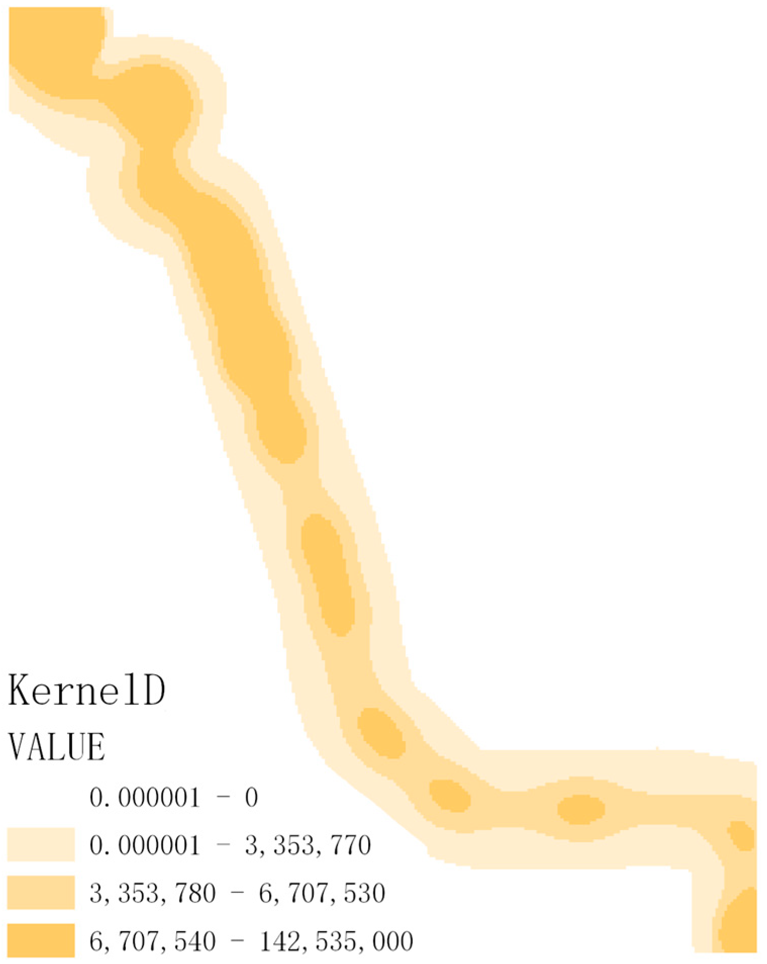
Nuclear density analysis is mainly used to build the track segment of a bus route in ArcGIS. By analyzing the density of carbon emissions in the adjacent estimated segments, a smooth and convex surface is created for the track point and makes it just at the highest position. The position gradually decreases with the increase in the distance from the point to zero.
The difference between the nuclear density analysis and the point density analysis is that the nuclear density analysis will increase the weight of the density center, making the high-density areas more concentrated and the low-density areas looser. Figure 2 shows the nuclear density analysis of a bus line in Sanya, and the density center of the density chart is relatively prominent. According to the data’s characteristics of the buses’ carbon emissions in Sanya, it is more convenient to select nuclear density analysis because it is difficult to distinguish the track point density charts among different lines, which cannot reflect the space–time characteristics of their carbon emissions.

4. Results and Discussions of the Spatial–Temporal Analysis of Carbon Emissions

4.1. Analysis of Time Characteristics for Carbon Emissions

This paper analyzes the GPS data of buses in Sanya from 15 to 21 March 2021, and calculates the CO2 emissions of 94 road sections in the study area in 37 statistical periods according to the calculation method of buses’ carbon emissions proposed in Section 3.3 with a 30 min statistical interval.

4.1.1. Comparative Analysis of Carbon Emissions in Different Periods

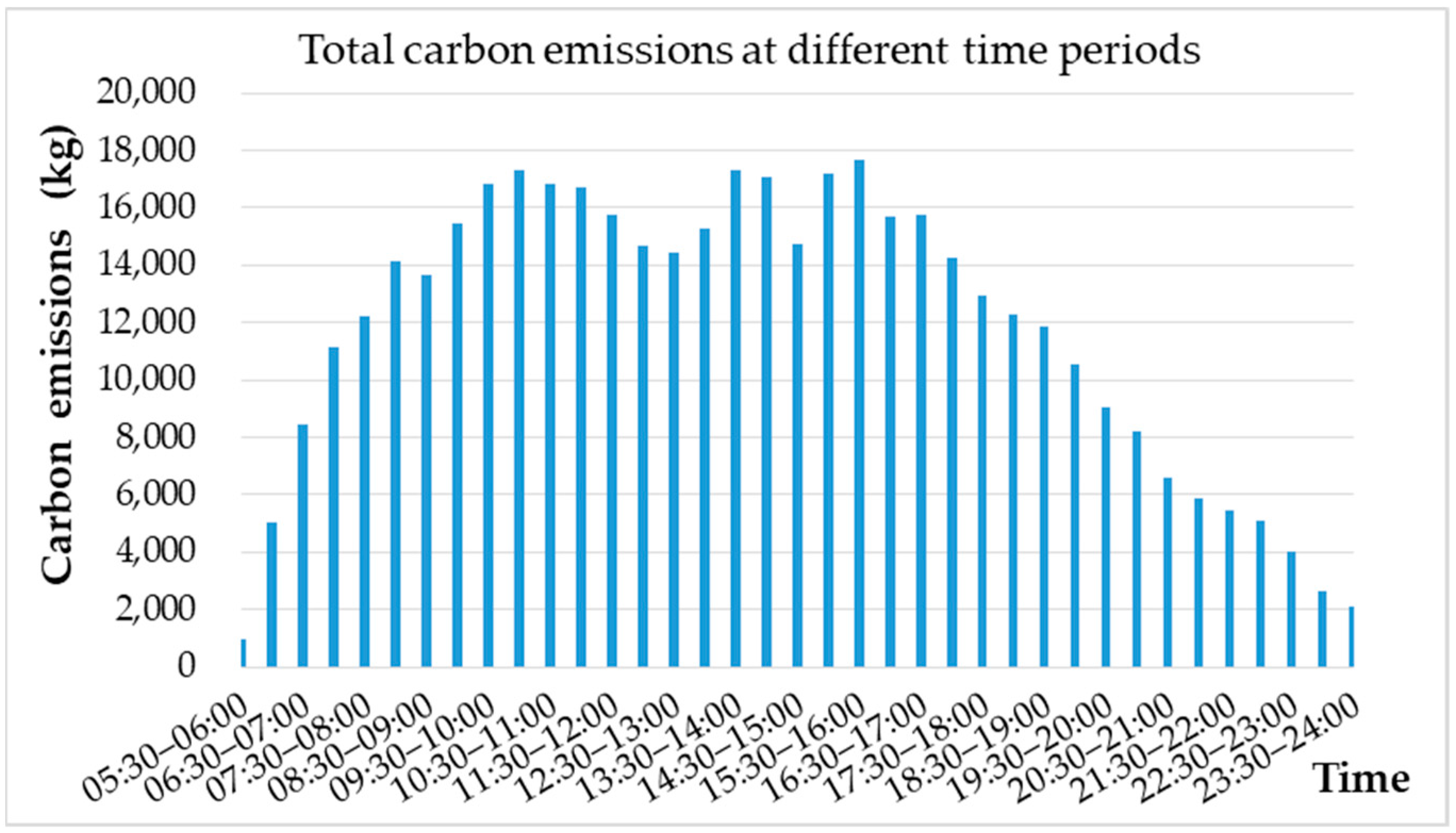
From Figure 3, we can clearly recognize the daily operational rules of buses in Sanya. According to the calculation data and research results, the information shown in the figure is consistent with people’s daily travel activities, and the number of buses and their carbon emissions are related in a day. Based on the buses’ operational schedule in Sanya, the time from 7:00 a.m. to 20:00 p.m. is their operational time. A few buses will operate until 12:00 a.m., but few will operate for 24 h. Therefore, the GPS data from 00:00 to 05:30 are removed as abnormal data in the calculation process, and the data from 05:30 to 24:00 are used for calculating the carbon emissions. After 6:00 in the morning, the buses start to operate, and their number increases gradually, about 750 buses starting to work. After 6:00 in the afternoon, the number of buses starts to decrease because of their operation time. Until 0:00 on the next day, the buses stop operating.
According to Figure 3, it can be found that the total carbon emissions are consistent with the buses’ operational time, and the lowest carbon emissions occur from 22:00 to 24:00. Before 12:00 every day, the emissions gradually rise, and then show a downward trend in the period from 12:00 to 14:00, because some buses will stop to rest. The emissions increase slightly from 14:00 to 16:00 and then tend to be stable. After 16:00 to 18:00 at the evening peak, the emissions begin to decline until the buses stop operation and the carbon emissions gradually turn to zero. According to the calculation, the daily CO2 emission of the buses in Sanya is about 65,000 tons.

4.1.2. Comparative Analysis of Carbon Emissions on Working Days and Rest Days

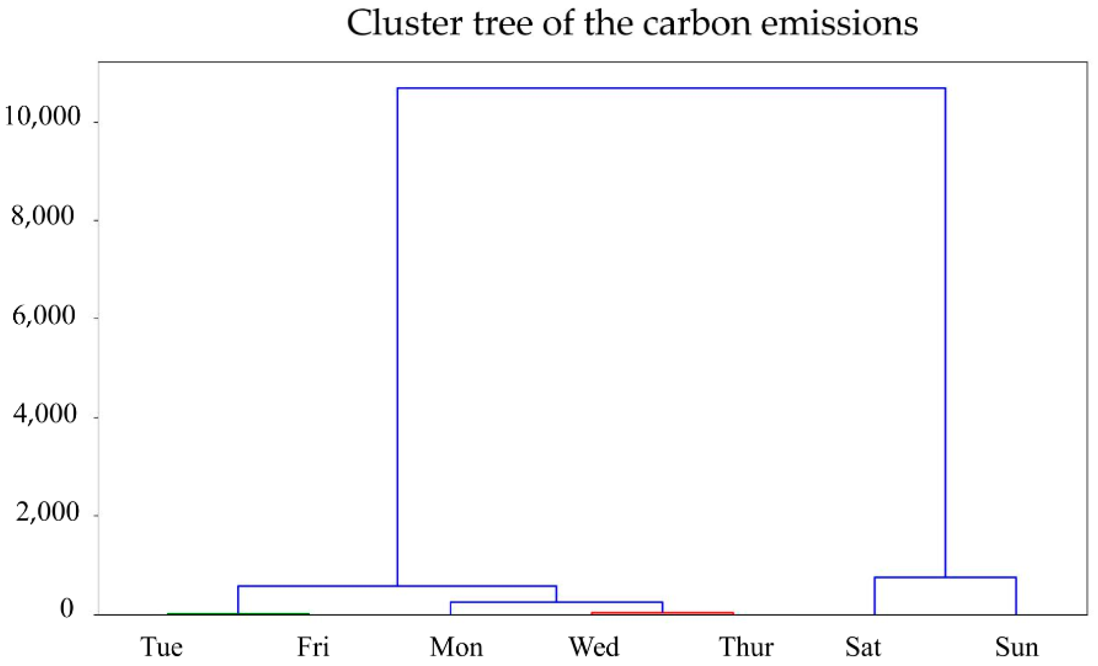
In order to observe the distribution of the carbon emissions for Sanya’s buses in different days of the week, the k-nearest neighbors algorithm is selected to carry on a cluster analysis to the CO2 emissions of Sanya’s buses in a week. According to Figure 4, the CO2 emissions show strong similarities on Monday and Friday, on Wednesday and Thursday, and the same clustering results on Saturday and Sunday.
At the same time, the similarity calculation of the buses’ carbon emission data in Sanya. According to Table 9, the similarity of CO2 emissions from Monday to Friday is above 0.95, while the data similarity between Saturday and Sunday is 0.989. Therefore, this paper divides the carbon emissions of Sanya’s buses into working days and rest days.
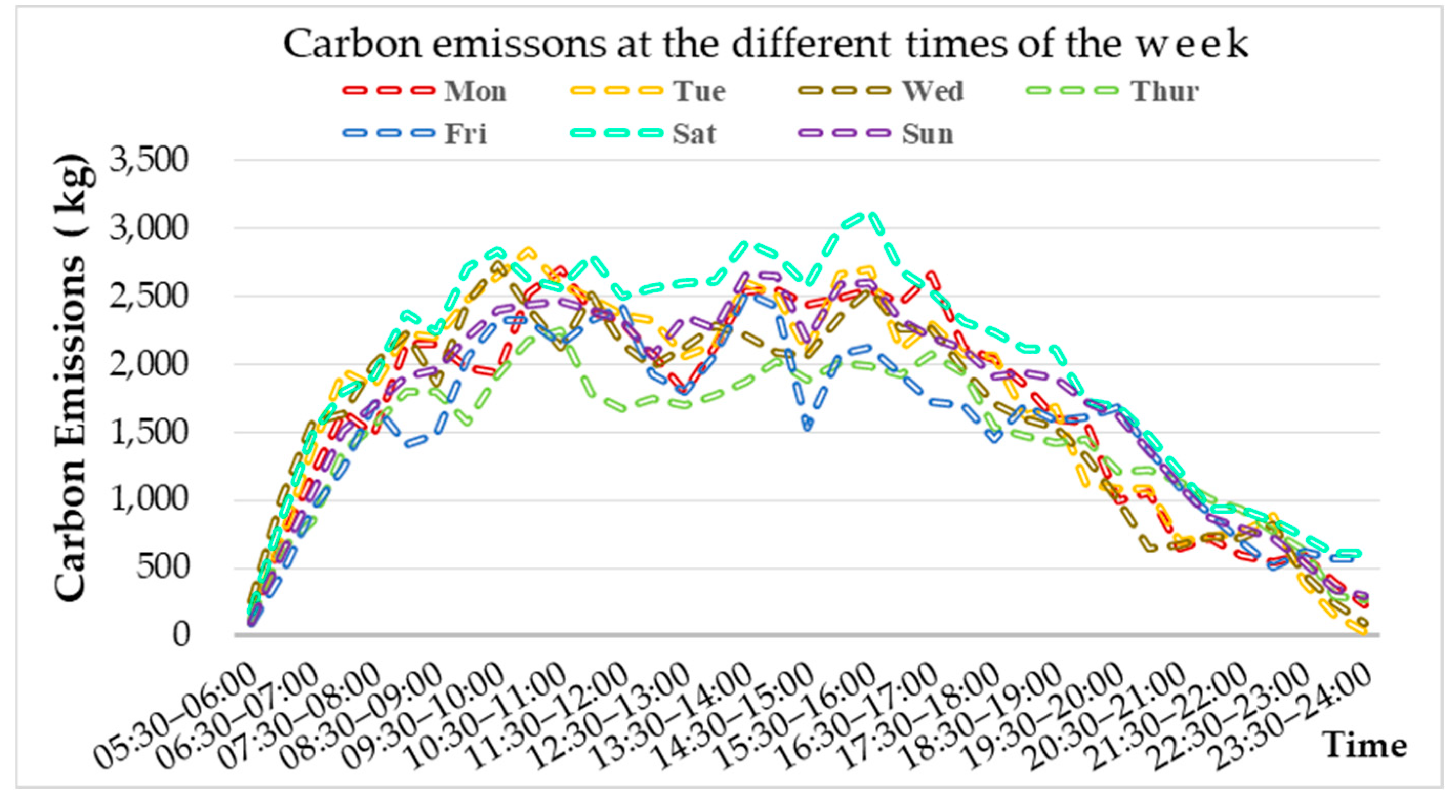
Carbon emissions of buses in Sanya during different periods of each working day and rest day are measured, and the results are shown in Figure 5. The CO2 emissions of buses on weekdays (Monday to Friday) is significantly higher in the morning and evening peak hours, and the carbon emission level is higher in the morning peak hours on the first three days of the week (7:30–9:30) and the evening peak hours on Friday (17:30–19:30) compared with the same time period on other days. The CO2 emissions of the remaining days showed strong similarity, and the carbon emissions decreased more at around 1:00 noon during the vehicle operation period. In general, the daily CO2 emission during working days is relatively stable, which is very similar to the characteristics of residents’ daily travel and bus schedule.
From Figure 5, it can be shown that there is a significant difference in the bus operational time between weekdays and weekends. Compared with weekdays, the carbon emissions of Sanya’s buses appear later in the morning peak, between 10:00 and 12:00 noon, and the change of carbon emissions is relatively gentle throughout the day. However, from the perspective of emission level, the emissions on Saturday are higher than those on Sunday.

4.1.3. Temporal Comparative Analysis of Carbon Emissions for Different Energy Types

By calculating the carbon emissions of different energy types of buses, the distribution in a day was statistically analyzed. Figure 6 and Figure 7 show the daily distribution of carbon emissions of buses in Sanya under different energy types on working days and rest days, respectively. From left to right, diesel, natural gas, and electricity are shown successively. From the perspective of total emissions, diesel is the highest, followed by electric vehicles, and natural gas is the smallest. This is because natural gas buses account for the smallest proportion of total buses, followed by diesel, and electric buses account for the highest proportion. In terms of unit emissions, electric buses have the smallest emissions, followed by natural gas, and diesel is the highest.
From Figure 6 and Figure 7, the overall change of carbon emissions of buses in different energy types is similar to that on working days and rest days, but there are significant differences in the fluctuations of different energy types, among which diesel buses’ emissions have the largest amplitude and electric buses’ emissions have the smallest amplitude. The reason for this is that different energy types have different carbon emission factors, and different types of buses have different energy consumptions per hundred kilometers, which makes diesel buses have higher emissions than other buses. Then, after 18:00 in the afternoon, the operation of natural gas buses gradually stops. The main operating buses on the line are diesel and natural gas buses, so the carbon emissions of electric buses are higher than that of natural gas buses.

4.2. Analysis of Spatial Characteristics of Carbon Emissions

4.2.1. Spatial Comparative Analysis of Carbon Emission on Working Days and Rest Days

In order to observe the distribution of buses’ carbon emissions in the road network in Sanya, the spatial distribution of carbon emissions in different periods of time is visualized and analyzed from working days and rest days, the carbon emission data are segmented at 2 h intervals, and the ArcGIS software is used to visualize them.
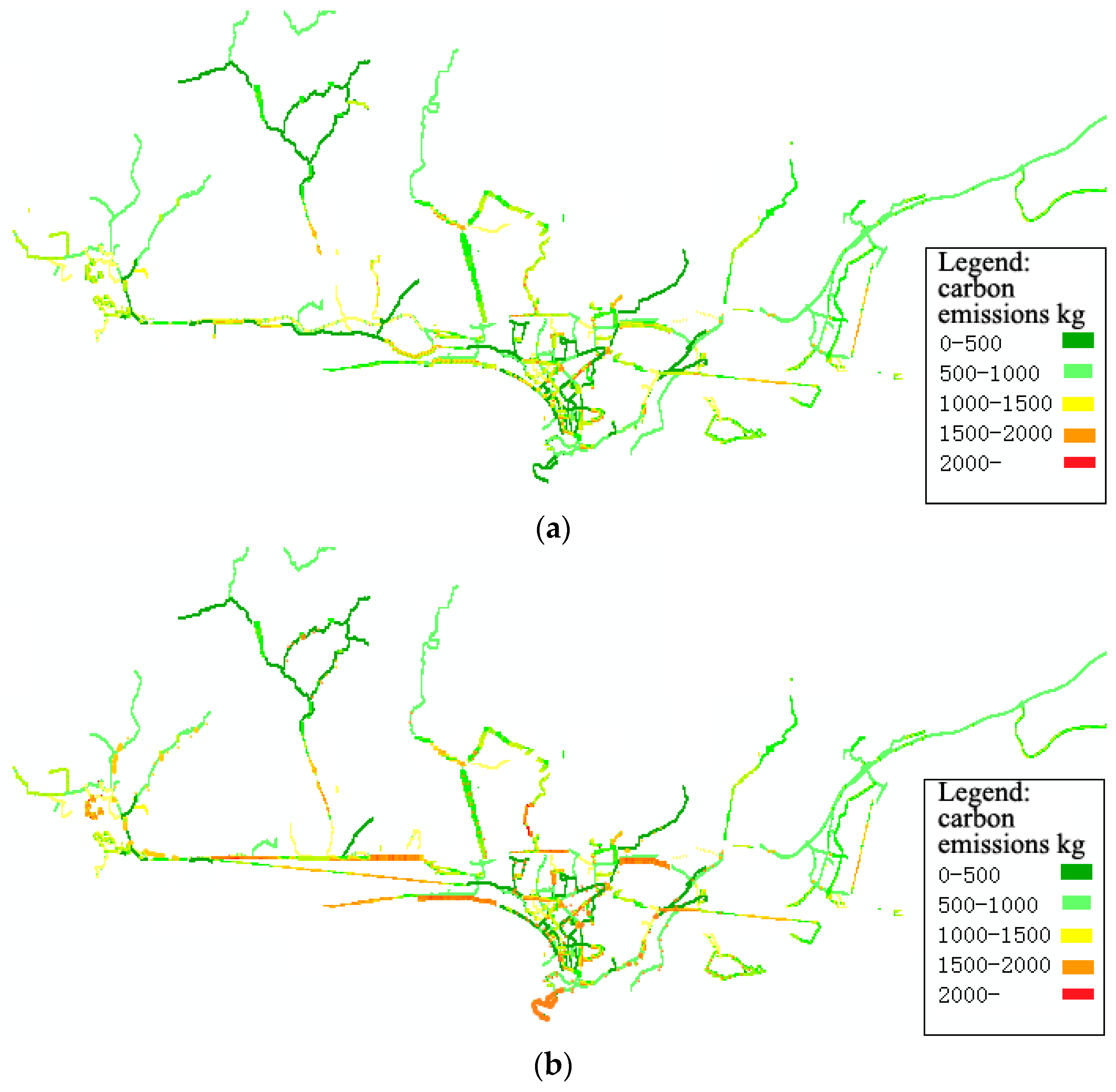
Figure 8 shows the spatial distribution of buses’ carbon emissions in Sanya at different times on the working days, mainly mapping the distributions of carbon emissions at 7:30–9:30 in the morning peak and at 17:30–19:30 in the evening peak. The map shows that the locations with high carbon emissions are mainly distributed in the urban center, and there are gathering areas of high emissions between Sanya Bay and coastal roads.
During the rush hours from 7:30 to 9:30 in the weekly mornings, the high-carbon emission areas of buses are mainly concentrated in the west of Sanya River Road, distributed in Jiefang Road, Shengli Road, Yingbin Street, and so on. Low-carbon roads are clustered outside the city center.
During the weekly evening peak from 17:30 to 19:30, the high-carbon emission zone increased compared with that in the morning time. In the downtown area, except for the west Sanya River Road, there were more high emissions in Xinfeng Street, Jixiang Street, Shuicheng Road, and so on. In the south, Sanya Bay Road has high-emission sections, mainly distributed in Shengli Road, South Hai Road, and Luling Road, and East Sanya River Road has relatively increased emission aggregation. New high carbon emissions occurred in the northern region, mainly in Linchun River Road and Xianghe Road. There are more areas with high carbon emissions in Hailuo First Road, Litchi East Road, Danzhou North Road, and Laoguoyuan Road, while those on Haihong Road and Lucheng Avenue are less.
Figure 9 shows the spatial distribution of urban buses’ carbon emissions in different periods of rest days. It can be clearly observed that the carbon emissions in the study area show a lower trend in the morning peak period. Compared with the distribution of carbon emissions on working days, the carbon emissions in the evening peak period show a more high-carbon emission distribution, which is similar to that in the evening peak period of working days, but there are more high-carbon emission areas. By comparing the spatial distribution of the carbon emissions at different times of the day, it is found that some areas are always at high-carbon emission levels at different times of the day, and these areas are mainly concentrated in urban centers, scenic sections, and transportation hub roads.
From 7:30 to 9:30 on weekends, there are fewer high-carbon emission zones than at other times of the day, mainly distributed in the south of Sanya River West Road and the north of Sanya Bay Road. From 17:30 to 19:30 on weekends, the areas with high carbon emissions are similar to those on weekdays, but the roads around the main business areas, such as Shengli Road, Xinfeng Street, Jiangang Road, and Jiefang Road, show more high carbon emissions. Around tourist attractions, such as Yalong Bay Road, Yingbin Road, Chunguang Road, Hongzhou Road, and Jinjiling Street, are high emissions too. In addition, Jiefang Road around Sanya Airport also has a lot of high-carbon emission sections.
The spatial distribution of buses’ carbon emissions in Sanya varies at different times. However, from the perspective of the overall distribution of the carbon emissions, the areas with high carbon emissions are mainly concentrated in downtown Sanya and the coastal sections, while the areas with low carbon emissions are concentrated in the inland areas of the city. The distribution of carbon emissions is consistent.

4.2.2. Spatial Comparative Analysis of Carbon Emissions on Different Lines

In order to visually show the differences of the routes of urban buses’ carbon emissions, the buses’ carbon emission is visualized by route track points.
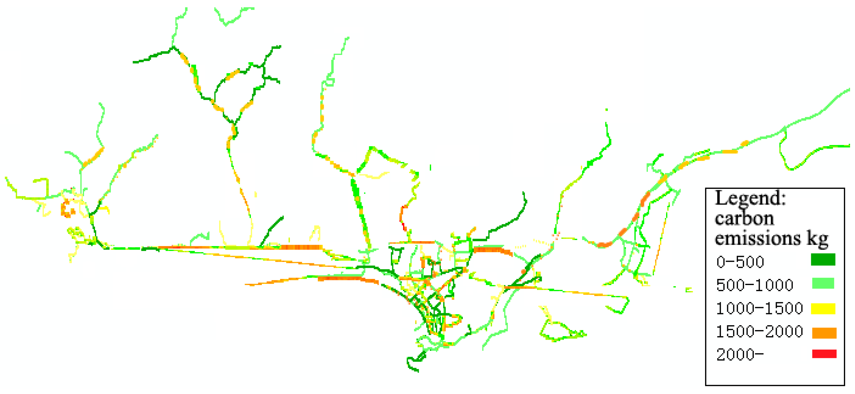
Figure 10 shows the spatial distribution of carbon emissions of buses on different routes on working days. The carbon emission data are all over the track points, the increasing trend of carbon emissions on routes is consistent with the change trend of total carbon emissions, the carbon emissions of urban fringe areas are low, those of urban central areas and transport hub sections are relatively high, and the CO2 emissions on routes on working days change significantly. There are about 58 lines with a carbon emission of less than 500 kg, 19 lines less than 1000 kg, 5 lines 1000–1500 kg, 5 lines 1500–2000 kg, and 7 lines more than 2000 kg. Most of the lines with high emissions are concentrated in Sanya Hexi Road of the city center, and the areas with a high overlap of bus lines, such as Xinfeng Street, Jixiang Street, Shuicheng Road, and other business districts and office areas, also have relatively high carbon emissions.
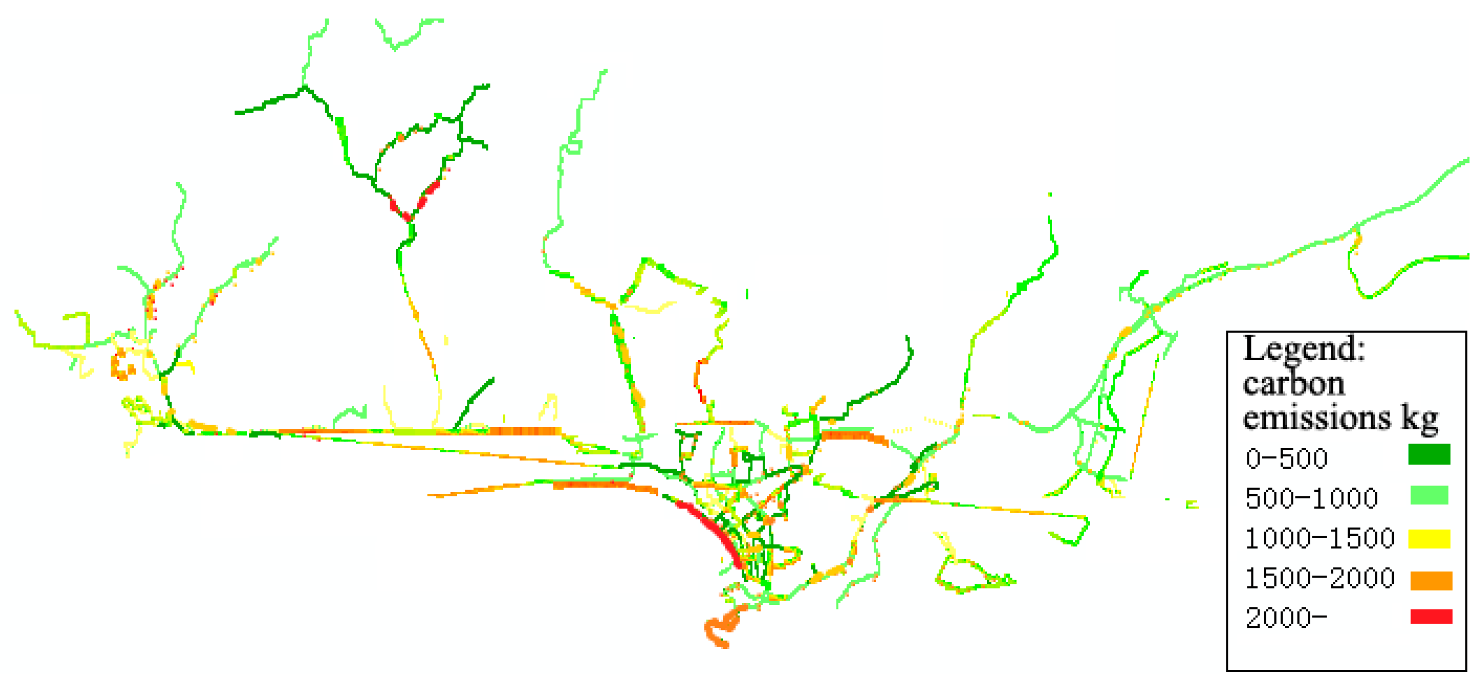
Figure 11 shows the spatial distribution of carbon emissions on different lines on rest days. There are 54 lines with carbon emissions of less than 500 kg, 19 lines less than 1000 kg, 7 lines 1000–1500 kg, 5 lines 1500–2000 kg, and 9 lines more than 2000 kg. Compared with workdays, most of the lines with high emissions are concentrated in urban central areas and business districts, and the carbon emissions of other lines are also higher than the same period of workdays. In addition, the bus lines’ emissions near coastal resort hotels are relatively high too.

5. Conclusions and Suggestions

5.1. Conclusions

This paper first divides the operating conditions of Sanya’s urban buses, adopts the methods of “distance × energy consumptions” to calculate the buses’ emissions in the driving process and adopts “time × energy consumptions” for calculating the idling condition, and calculates the total carbon emissions of Sanya’s urban buses in a week of operation. Second, the spatial and temporal distributions of buses’ carbon emissions in Sanya are visualized to provide some data support for the formulation of efficient and reasonable policies on carbon emission reduction.
  • By using the data of GPS track and buses’ management of Sanya’ urban buses, this paper combines the energy consumption attributes, operating conditions, and buses’ emission models to achieve the calculation of buses’ CO2 emissions at different track points in a day. Through the calculation, the spatial–temporal distribution of urban buses’ carbon emissions can be more accurately excavated.
  • After visualizing the temporal and spatial distribution characteristics of buses’ carbon emissions in Sanya, it is found that from the temporal perspective, the distribution of buses’ carbon emissions at different times of the day in a week is similar to the daily travel characteristics of residents. The carbon emissions at the peak time are significantly higher than the off-peak time, and there will also be peak bands. Compared with the weekdays, the morning peak on the weekend occurs later, and the change of carbon emissions is relatively stable within a day. Through the analysis of different energy types of buses in different periods, it is found that the carbon emissions of natural gas and diesel buses are significantly higher than those of electric buses in the daytime, and the carbon emissions of diesel and electric buses are higher than those of natural gas buses after 18:00 p.m. From the perspective of space, the distribution of carbon emissions in different time periods during the weekdays and the weekends is also different. The road sections with higher carbon emissions are mainly concentrated in residential areas, offices, and schools in the early peak period, and mainly in leisure and entertainment areas in the late peak period. The carbon emissions on different lines are also different in the spatial distribution. The lines with high station density are mostly concentrated in the central area of the city, and their emissions are higher than those with low station density and distributed at the edge of the city.

5.2. Suggestions

Based on the research conclusions of this paper, suggestions on the policies of reducing the carbon emissions of urban buses are mainly put forward from the following two aspects, so as to better develop the urban buses’ operation towards green and low-carbon travel, and further control the carbon emissions of the transport industry:
  • Optimize the energy structure of buses
Through the research results of this paper, it is found that the carbon emissions of electric buses in different energy types of buses are the lowest, which also conforms to the fact that the reduction of energy consumptions can promote the reduction of carbon emissions. Therefore, it is necessary to accelerate the proportion of new energy buses in urban buses and promote low-carbon operation of green transport. Increase support for the introduction of new energy vehicles in policy. Arrange incentive funds to encourage the purchase and use of new energy vehicles through incremental control of diesel vehicles; in the process of vehicles’ operation, increase the operating subsidies for new energy buses, and implement preferential policies for charging prices.
  • Optimize the layout of buses’ network
Different arrangements shall be made for buses’ operation in different periods. According to the characteristics of buses’ operation in peak and off-peak periods, the number of buses on lines shall be reasonably adjusted, and the departure interval shall be optimized to minimize congestion in peak periods. Through the trunk line, it can effectively replace the repeated lines at bus stops and reduce unnecessary energy waste caused by the repeated lines; through the reasonable design for buses’ lines, reduce detours, delays, and other situations; through the optimization of bus stops, the horizontal and vertical separation of bus stops with concentrated lines, reduce the arrival time and ease the problem of difficult arrival during peak hours.

Author Contributions

Conceptualization, Y.L., C.Z. (Changzheng Zhu) and C.Z. (Cong Zhang); methodology, Y.L., C.Z. (Changzheng Zhu) and C.Z. (Cong Zhang); software, Y.L. and C.Z. (Cong Zhang); validation, C.Z. (Changzheng Zhu); formal analysis, Y.L., C.Z. (Changzheng Zhu) and C.Z. (Cong Zhang); investigation, Y.L., C.Z. (Changzheng Zhu) and C.Z. (Cong Zhang); resources, Y.L., C.Z. (Changzheng Zhu), C.Z. (Cong Zhang) and R.P.; data curation, Y.L., C.Z. (Changzheng Zhu), C.Z. (Cong Zhang) and R.P.; writing—original draft preparation, Y.L., C.Z. (Changzheng Zhu), C.Z. (Cong Zhang) and R.P.; writing—review and editing, Y.L. and C.Z. (Changzheng Zhu); visualization, Y.L. and C.Z. (Changzheng Zhu); supervision, Y.L. and C.Z. (Changzheng Zhu); project administration, Y.L. and C.Z. (Changzheng Zhu); funding acquisition, Y.L. and C.Z. (Changzheng Zhu). All authors have read and agreed to the published version of the manuscript.

Funding

This research was funded by the Philosophy and Social Sciences Major Theoretical Issues Research Project of Shaanxi Province, grant number 2022ND0165, and Soft Science Research Project of Xi’an Science and Technology Plan, grant number 22RKYJ0040.

Institutional Review Board Statement

Not applicable.

Informed Consent Statement

Not applicable.

Data Availability Statement

Not applicable.

Acknowledgments

The authors thank Lijiao Qin for her help in the English editing.

Conflicts of Interest

The authors declare no conflict of interest.

References

  1. Zhu, J.; Liu, X.M.; Chu, Z.P. Analysis on the development ways of urban low-carbon transportation. Ecol. Econ. 2016, 32, 76–81. [Google Scholar]
  2. Long, Y.; Sun, L.J.; Tao, S. Literature review on urban buses’ data of smart card. Urban Plan. Forum. 2015, 03, 70–77. [Google Scholar]
  3. Sun, Z.; Hao, P.; Ban, X.J.; Yang, D. Trajectory-based vehicle energy/emissions estimation for signalized arterials using mobile sensing data. Transp. Res. Part. D Transp. Environ. 2015, 34, 27–40. [Google Scholar] [CrossRef]
  4. Luo, X.; Dong, L.; Dou, Y.; Zhang, N.; Ren, J.; Li, Y.; Sun, L.; Yao, S. Analysis on spatial-temporal features of taxis’ emissions from big data informed travel patterns: A case of Shanghai, China. J. Clean. Prod. 2016, 142, 926–935. [Google Scholar] [CrossRef]
  5. Du, Y.; Wu, J.; Yang, S.; Zhou, L. Predicting vehicle fuel consumption patterns using floating vehicle data. J. Environ. Sci. 2017, 59, 24–29. [Google Scholar] [CrossRef]
  6. Weng, J.C.; Liang, Q.; Qiao, G.L.; Chen, Z.H.; Rong, J. Taxi fuel consumption and emissions estimation model based on the reconstruction of driving trajectory. Adv. Mech. Eng. 2017, 9, 209–216. [Google Scholar] [CrossRef]
  7. Shan, X.N.; Chen, X.H.; Jia, W.J.; Ye, J.H. Evaluating urban bus emission characteristics based on bocalized MOVES using sparse GPS Data in Shanghai, China. Sustainability 2019, 11, 2936. [Google Scholar] [CrossRef] [Green Version]
  8. Sui, Y.; Zhang, H.R.; Shang, W.L.; Sun, R.C.; Wang, C.Y.; Ji, J.; Song, X.; Shao, F.J. Mining urban sustainable performance: Spatio-temporal emission potential changes of urban transit buses in post-COVID-19 future. Appl. Energy 2020, 280, 115966. [Google Scholar] [CrossRef]
  9. Zhou, Y.; Huang, R.H.; Tang, E.B. Dynamic calculation method of carbon emissions of urban road traffic based on GPS+GIS+ GSM. J. Nanchang Hangkong Univ. (Soc. Sci.) 2016, 18, 35–41. [Google Scholar]
  10. Guo, Y.Y. Research on Emission Factors of Motor Vehicles in Shenzhen Based on MOVES Model. Master’s Thesis, Harbin Institute of Technology, Harbin, China, 2014. [Google Scholar]
  11. Niu, T.L. Research on Emission Inventory of High-Resolution Road Network in Nanjing Based on Intelligent Transportation Big Data. Master’s Thesis, Tsinghua University, Beijing, China, 2017. [Google Scholar]
  12. Xu, L.; Wang, L.; Liu, Y.; Song, G.H.; Li, C.X.; Zhai, Z.Q. Calculation model of buses’ energy consumptions and carbon emissions based on multi-source data. J. Transp. Syst. Eng. Inf. Technol. 2020, 20, 174–181. [Google Scholar]
  13. Andrienko, G.; Andrienko, N. Spatio-temporal Aggregation for Visual Analysis of Movements. In Proceedings of the IEEE Symposium on Visual Analysis Science and Technology, Columbus, OH, USA, 19–24 October 2008; pp. 51–58. [Google Scholar] [CrossRef] [Green Version]
  14. Nam, D.; Hyun, K.; Kim, H.; Ahn, K.; Jayakrishna, R. Grid Cell Based Taxi Ridership Analysis Using Large Scale GPS Data. In Proceedings of the Transportation Research Board 95th Annual Meeting, Washington, DC, USA, 10–14 January 2016. [Google Scholar]
  15. Zhao, P.; Kwan, M.P.; Qin, K. Uncovering the spatiotemporal patterns of CO2 emissions by taxis based on Individuals’ daily travel. J. Transp. Geogr. 2017, 62, 122–135. [Google Scholar] [CrossRef]
  16. Wang, Z.H. Research on Spatial and Temporal Accessibility Distribution of Urban Multimodal Traffic. Master’s Thesis, Shenzhen University, Shenzhen, China, 2016. [Google Scholar]
  17. Xu, Y.J. Analysis of Spatial-Temporal Characteristics of Residents’ Travel Based On Taxi Track Data. Master’s Thesis, Shandong University of Science and Technology, Qingdao, China, 2017. [Google Scholar]
  18. Wang, G.; Sun, Y.L.; Wang, X.Z.; Li, J.Z. Analysis and application of spatial-temporal characteristics of transportation in Wuhan City based on typical dynamic data. Traffic Transp. 2019, 35, 29–32. [Google Scholar]
  19. Zheng, M.L.; Yang, H.L. Spatial-temporal changes and factors of carbon emissions from cargo transport at the municipal scale. Sci. Surv. Mapp. 2019, 05, 76–84. [Google Scholar]
  20. Ning, X.J.; Zhang, J.P.; Qin, Y.C.; Lu, F.X. Temporal and spatial characteristics of urban residents’ traffic carbon emissions in Zhengzhou. Resour. Sci. 2014, 36, 1021–1028. [Google Scholar]
  21. Sun, G.J. Characteristics and Emission Reduction Measures of PM2.5 and NOX from Motor Vehicles. Doctoral Thesis, Zhejiang University, Hangzhou, China, 2013. [Google Scholar]
  22. Gao, Z.F. Study on the Coordinated Treatment of Carbon Emissions and Air Pollution Emissions in the Yangtze River Delta Urban Agglomeration. Master’s Thesis, Zhejiang University of Technology, Hangzhou, China, 2019. [Google Scholar]
  23. Schipper, L.; Grubb, M. On the rebound feedback between energy intensities and energy uses in IEA countries. Energy Policy 2000, 28, 367–388. [Google Scholar] [CrossRef]
  24. Sun, J.; Zhang, Y.; Xue, R.; Zhang, Y. Formation mechanism of carbon emission from urban road traffic based on mobile monitoring: A case study of Shanghai. China J. Highw. Transp. 2017, 30, 122–131. [Google Scholar]
  25. Halevi, G.; Moed, H. The evolution of big data as a research and scientific topic: Overview of the literature. Res. Trends 2012, 30, 3–6. [Google Scholar]
  26. Hey, T.; Gannon, D.; Pinkelman, J. The future of data-intensive science. Computer 2012, 45, 81–82. [Google Scholar] [CrossRef]
  27. Dong, Y. Research on dynamic visualization of buses’ GPS track based on Web. Innovative technology Enabling planning Wisdom for the Future. In Proceedings of 2021 China Urban Planning Informatization Annual Conference, Online conference, 10 December 2021; pp. 138–143. [Google Scholar] [CrossRef]
  28. Wang, X. Research on Key Problems of Urban Taxi Operation Service Based On Large Scale GPS Data. Doctoral Dissertation, Jilin University, Changchun, China, 2021. [Google Scholar]
  29. Zhao, Z.X.; Shao, C.F.; Chen, Y. Assessment of carbon emission reduction effect of private electric cars in the Whole Life Cycle in Chinese Provinces. J. Henan Sci. Technol. 2021, 34, 2076–2085. [Google Scholar]
  30. Chu, R.S.; Wu, T.L.; He, W.C.; Cao, G.H. Research on carbon-emission model of toll stations of expressways under dual carbon targets. J. Henan Sci. Technol. 2021, 40, 120–123. [Google Scholar]
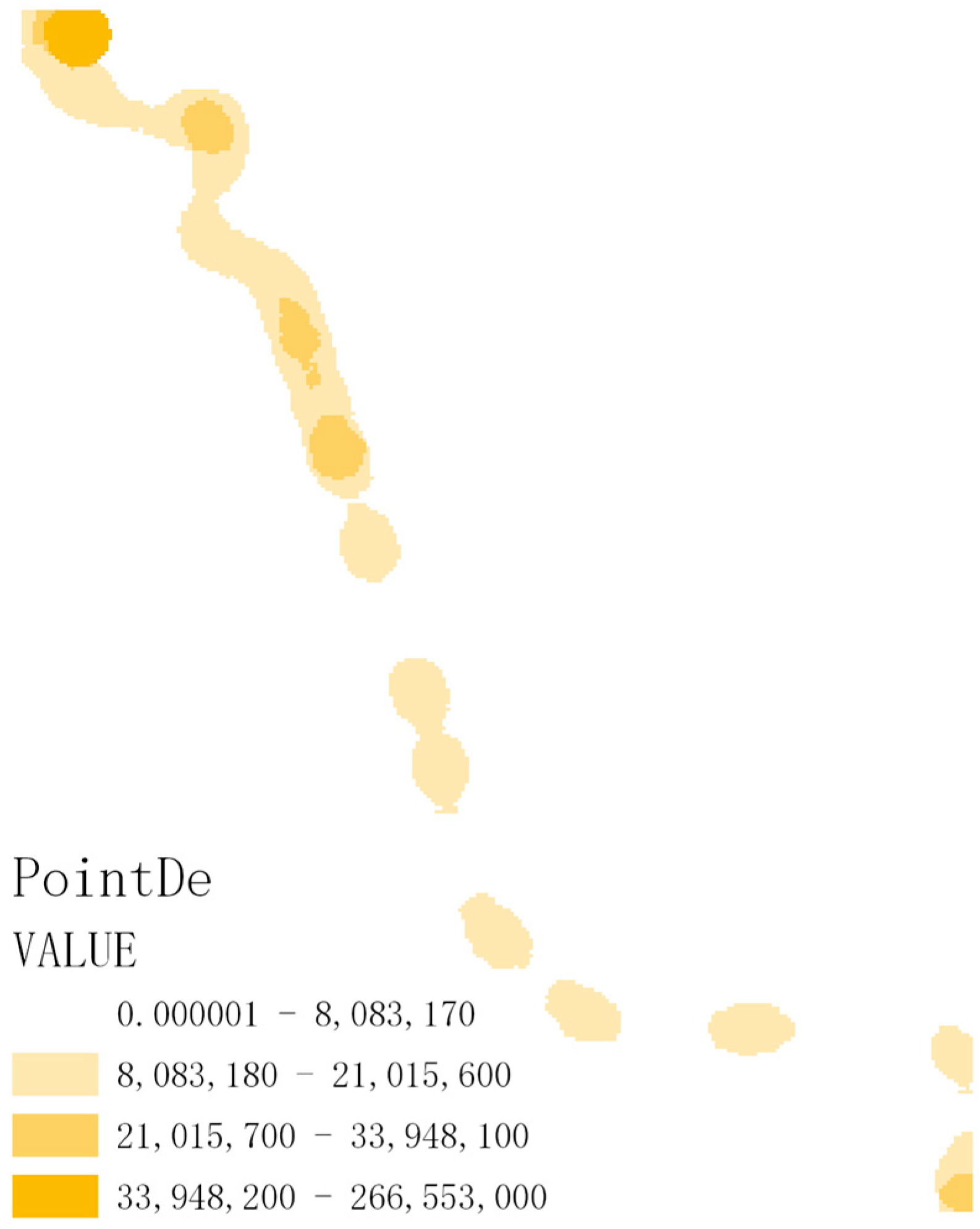
Figure 1. Analysis of point density.
Atmosphere 14 00411 g001
Figure 2. Analysis of nuclear density.
Atmosphere 14 00411 g002
Figure 3. Time span of the emissions for the buses in Sanya.
Atmosphere 14 00411 g003
Figure 4. Cluster tree of the carbon emissions for the buses in Sanya.
Atmosphere 14 00411 g004
Figure 5. Time distribution of buses’ carbon emissions in Sanya of the week.
Atmosphere 14 00411 g005
Figure 6. Time distribution of different types of energy type buses’ carbon emissions in Sanya on weekdays. (a) Total carbon emissions of vehicles with different energy types on weekdays. (b) Carbon emissions of one vehicle with different energy types on weekdays.
Atmosphere 14 00411 g006
Figure 7. Time distribution of different types of buses’ carbon emissions in Sanya on rest days. (a) Total carbon emissions of vehicles with different energy types on rest days. (b) Carbon emissions of one vehicle with different energy types on rest days.
Atmosphere 14 00411 g007
Figure 8. Spatial distribution of buses’ carbon emissions in Sanya on weekdays. (a) Spatial distribution of carbon emissions in the morning. (b) Spatial distribution of carbon emissions in the evening peak.
Atmosphere 14 00411 g008
Figure 9. Spatial distribution of buses’ carbon emissions in Sanya on rest days. (a) Spatial distribution of the carbon emissions in the morning peak. (b) Spatial distribution of carbon emissions in the evening peak.
Atmosphere 14 00411 g009
Figure 10. Spatial distribution of carbon emissions on buses lines in Sanya on weekdays.
Atmosphere 14 00411 g010
Figure 11. Spatial distribution of carbon emissions on buses lines in Sanya on rest days.
Atmosphere 14 00411 g011
Table 1. Illustration of the GPS data.
No.Field NameIllustrationExample
1GPS acquisition timeAcquisition time of GPS data (accurate to one track point every 6 s)15 March 2021 09:03:20:000
2Longitude Longitude coordinate of current buses’ operation109.16589884507853
3Latitude Latitude coordinate of current vehicle operation18.370064237983335
4Speed Instantaneous running speed of vehicle (km/h)19.00
5Equipment line no. Running lines for buses501
6Equipment no.Numbers of buses532
7Station sequence Bus stops’ ordinal3
8Type of pulling in and out1: pull in 2: pull out1
Table 2. Illustration of buses’ characteristic data.
No.Field NameIllustrationExample
1Self-numberCorresponding equipment number in the GPS data, namely, numbers of buses532
2Types of energiesIncluding: diesel, natural gas, electricDiesel
3Engine numberThe engine models of the current busesFGGJAG00744
4Length of busesLength of the current buses (length × width × height mm)5990 × 2250 × 2995
5License plateThe brands of busesBrand of Ankai
Table 3. Data illustration of buses’ routes.
No.Field NameIllustrationExample
1Name of routeNames of buses’ routes Route 1
2Starting stationStarting station of current routePort office
3Terminal Terminal of current route Tropical Ocean University
4Names of stationName of the station of the current running busYifang Department Store
5Station’s sequence Sequence of the current on-line station3
Table 4. Buses’ operational states in Sanya.
Upload Time of GPSLongitudeLatitudeSpeed
(km/h)
Stations’ No.Types of Inbound and OutboundStates of Vehicles
15 March 2021 08:12:19:000109.1738765095295218.3509827367548922.002112
15 March 2021 08:12:25:000109.1738580924603218.3510361963875522.00 2
15 March 2021
08:12:31:000
109.1737616745385818.3513346897827919.00 2
15 March 2021
08:12:37:000
109.1737267372762418.351457876933100.00 1
15 March 2021
08:12:43:000
109.1737267372762418.351457876933100.00 1
15 March 2021
08:12:49:000
109.1737267372762418.351457876933100.00 1
15 March 2021
08:12:55:000
109.1737267372762418.351457876933100.00 1
15 March 2021
08:13:01:000
109.1737267372762418.351457876933100.00 1
15 March 2021
08:13:07:000
109.1737251128774318.351476321015557.00 2
15 March 2021
08:13:13:000
109.1736419638160818.3516880081027120.00 2
15 March 2021
08:13:19:000
109.173505459230518.3520516636651423.002122
Table 5. Carbon emission coefficient of transportation energy.
EnergyConversion Coefficient to Standard Coal (kg/kg, m3)Average Low Calorific Value (kJ/kg, m3)Carbon Content per Unit Calorific Value (kg-c/GJ)Carbon Oxidation Rate
(%)
Carbon Emission Coefficient (kg-CO2 or kg-CO2/m3)
Raw coal0.714320,90826.370.941.9003
Diesel oil1.457142,65220.20.983.0959
Natural gas1.3338,93115.320.992.1650
power-----
Data source: IPCC, version 2006.
Table 6. Relevant parameters of diesel bus brands.
No. Brand Percentage Length (mm)Energy Consumption per 100 km (L/100 km)
1Ankai 25.53%5990 × 2250 × 299514
2Ankai 2.43%9995 × 2500 × 322028
3Golden Dragon2.74%10,990 × 2500 × 360018.7
4Golden Dragon27.05%10,510 × 2500 × 330014.3
5Yutong3.04%6610 × 2240 × 299018
6Yutong2.43%10,185 × 2500 × 322025.5
7Kinglong3.04%8495 × 2480 × 338818.5
8Kinglong5.47%10,490 × 2480 × 340420.6
9Kinglong5.17%10,500 × 2500 × 337018.5
10Kinglong23.10%10,700 × 2500 × 330016.9
Table 7. Relevant parameters of electric buses of different brands.
No. Brand Percentage Length (mm)Energy Consumption per 100 km (kwh/100 km)
1Ankai3.78%10,990 × 2500 × 359054.64
2Kinglong4.72%8545 × 2450 × 314538.76
3CRRC6.46%10,500 × 2500 × 328053.00
4BYD14.65%10,690 × 2500 × 358044.08
5BYD4.41%4460 × 1720 × 187513.97
6Winnerway11.34%8560 × 2410 × 308038.67
7Winnerway4.72%10,450 × 2480 × 322051.68
8Skywell3.15%8010 × 2160 × 286038.68
9Skywell1.57%8490 × 2460 × 312044.30
10Zhongtong 2.52%6645 × 2280 × 300028.20
11Zhongtong 1.89%8600 × 2489 × 328037.79
12Zhongtong 5.20%10,480 × 2500 × 328052.73
13Yutong5.35%6395 × 2065 × 293030.66
14Yutong8.50%8050 × 2350 × 310546.83
15Yutong 3.15%8995 × 2500 × 345042.57
16Yutong10.71%10,500 × 2500 × 321554.81
17Yutong6.30%10,690 × 2500 × 343052.36
18Yutong 1.57%12,300 × 2550 × 414064.83
Table 8. Energy consumption of natural gas for different brands of buses.
No. Brand Percentage Length of the Brand (mm)Energy Consumption of LNG per 100 km (kg/100 km)Energy Consumption of LNG of per 100 km
(L/100 km)
1Yutong20.26%8545 × 2500 × 320027.4561.00
2Yutong3.92%9295 × 2500 × 320032.0871.29
3Yutong6.54%10,490 × 2500 × 355032.0871.29
4Yutong13.07%10,490 × 2500 × 358032.0871.29
5Yutong24.83%10,500 × 2500 × 320032.0871.29
6Ankai24.83%5900 × 2250 × 299521.1847.07
7Kinglong6.54%8490 × 2450 × 308027.4561.00
Table 9. Similarity matrix of carbon emissions of Sanya’s buses.
MonTueWedThuFriSatSun
Monday1.0000.9950.9810.9930.9720.8760.815
Tuesday0.9951.0000.9850.9980.9840.9110.855
Wednesday0.9810.9851.0000.9870.9660.9230.879
Thursday0.9930.9980.9871.0000.9880.9190.867
Friday0.9720.9850.9660.9881.0000.9350.890
Saturday0.8760.9110.9230.9190.9351.0000.989
Sunday0.8150.8550.8790.8670.8900.9891.000
Disclaimer/Publisher’s Note: The statements, opinions and data contained in all publications are solely those of the individual author(s) and contributor(s) and not of MDPI and/or the editor(s). MDPI and/or the editor(s) disclaim responsibility for any injury to people or property resulting from any ideas, methods, instructions or products referred to in the content.