Article

Continuous Measurements and Source Apportionment of Ambient PM2.5-Bound Elements in Windsor, Canada

1
Department of Civil and Environmental Engineering, University of Windsor, Windsor, ON N9B 3P4, Canada
2
Ontario Ministry of the Environment, Conservation and Parks, Toronto, ON M9P 3V6, Canada
*
Author to whom correspondence should be addressed.
Atmosphere 2023, 14(2), 374; https://doi.org/10.3390/atmos14020374
Submission received: 23 November 2022 / Revised: 6 February 2023 / Accepted: 9 February 2023 / Published: 14 February 2023
(This article belongs to the Special Issue The Michigan-Ontario Ozone Source Experiment (MOOSE))

Abstract

:
Ambient fine particulate matter (PM2.5) levels in Windsor, Ontario, Canada, are impacted by local emissions and regional/transboundary transport input and also attributable to secondary formation. PM2.5-bound elements were monitored hourly in Windsor from April to October 2021. Observed concentrations of the elements were generally comparable to historical measurements at urban sites in Ontario. A clear diurnal pattern was observed for most of the elements, i.e., high in the morning and low in the afternoon, mostly related to evolution of atmospheric mixing heights and local anthropogenic activities. Conversely, sulfur showed elevated levels in the afternoon, suggesting conversion of gaseous sulfur dioxide to particulate sulphate was enhanced by increased ambient temperatures. Five source factors were resolved using the US EPA positive matrix factorization model, including three traffic-related sources (i.e., vehicular exhaust, crustal dust, and vehicle tire and brake wear factors) and two industrial sources (i.e., coal/heavy oil burning and metal processing factors). Overall, the three traffic-related sources were mostly local and contributed to 47% of the total elemental concentrations, while the two industrial sources may originate from regional/transboundary sources and contributed to 53%. Measures to control both local traffic emissions and regional/transboundary industrial sources would help reduce levels of PM2.5-bound elements in Windsor.

1. Introduction

Fine particulate matter (PM2.5) refers to particles in the air with aerodynamic diameter less than 2.5 μm. PM2.5 sources include industrial activities, transportation, residential wood burning, and forest fires [1]. PM2.5 is also formed by the reactions of gas phase precursors in the air. In Ontario, Canada, its major components include sulphate, nitrate, organic matter, black carbon (BC), trace elements, and air toxics [2,3]. Jeong et al. [4] reported that, on average, sulphate, nitrate, organic matter, elemental carbons, and crustal matter accounted for 23%, 22%, 24%, 8%, and 5% of annual PM2.5 concentrations, respectively, in Toronto, Ontario, between 2004 and 2017.
PM2.5 is associated with various health effects, such as respiratory and cardiovascular diseases, lung cancer, adverse reproductive and developmental effects, neurological effects, and mortality [5]. Airborne particulate matter is considered carcinogenic to humans according to the International Agency for Research on Cancer [5]. Exposure to PM2.5 remains a health concern since there is no clear evidence of a population threshold below which health effects are not observed at ambient concentrations in Canada [6]. Identifying probable sources and their relative contributions is important to develop control measures to reduce PM2.5 emissions and ambient levels in the area.
Windsor is a city in southwestern Ontario, Canada, directly across from Detroit, Michigan, US. PM2.5 levels in Windsor are impacted by local emissions and transboundary transport input [2,7]. Local sources include industrial emissions of PM2.5 and metals [7], as well as road traffic. PM2.5 can also travel a long distance and affects its regional levels. Dominant winds in Windsor are from the south and southwest, downwind of neighboring US states where there are many industrial emission sources of PM and its precursors. A recent modelling study estimated that transboundary sources (mainly secondary PM2.5) contribute to over 70% of annual PM2.5 in Windsor [7]. Although PM2.5 levels have decreased over the past ten years, Windsor reported the 2nd highest PM2.5 Canadian Ambient Air Quality Standard (CAAQS) metric values in 2019 (i.e., 20 µg/m3 for the 24 h CAAQS metric and 8.1 µg/m3 for the annual metric) among the 24 monitoring stations in Ontario, Canada. In addition to long-term monitoring of PM2.5, levels of PM2.5-bound species have been monitored in Windsor through an integrated method that collects air samples over a 24 h period once every 6th day under the National Air Pollution Surveillance program [8,9]. The speciation measurements provided insights into the relative contributions of different components to PM2.5 and were further used to identify source factors impacting PM2.5 levels in Windsor. Emissions of PM2.5 and its major components vary temporally due to changes in industrial and human activities, as well as local meteorology. The 24 h integrated measurements revealed how levels of PM2.5 and its major components vary seasonally and annually. However, the 24 h integrated samples are unable to provide diurnal variability information that is useful for the identification of local emission sources [10,11].
During the Michigan–Ontario Ozone Source Experiment (MOOSE) study in the summer of 2021, extensive field work was carried out to improve the understanding of air pollution in the border community. Air monitoring in Windsor was enhanced through the collection of continuous hourly measurements of PM2.5-bound elements to support the MOOSE study, with concurrent hourly measurements of PM2.5 and BC also collected [3,12]. The hourly data of these species allow for assessment of diurnal patterns and the impacts of local and regional sources. This unique set of hourly measurements for trace elements, PM2.5, and BC was further used to determine major source types and their relative contributions by employing the US EPA Positive Matrix Factorization (PMF) model [13]. The objectives of this study were to assess ambient levels and the temporal variations of trace elements in Windsor and to identify the potential source sectors of trace elements and their relative contributions.

2. Methodology

2.1. Data Collection

Concentrations of ambient PM2.5, BC, PM2.5-bound elements, and meteorological parameters (i.e., temperature, wind direction, and wind speed) were monitored hourly across three seasons (i.e., spring, summer, and fall) from April to October 2021 at Windsor West station (42.29° N, 83.07° W), as shown in Figure 1. Spring is from April to May, summer is from June to August, and fall is from September to October. The station is surrounded by green space and two-story residential buildings. It is located 0.9 km southwest of Huron Church Road and 2 km south of the Ambassador Bridge, the busiest international border crossing in North America [14]. Approximately 2.6 million heavy-duty trucks and 4.6 million passenger vehicles crossed the bridge in 2018 [15]. In addition, the station is 3.5 km northeast of Zug Island (Figure 1), a heavily industrialized island that releases the largest amount of SO2 emissions in Michigan [16].
Hourly concentrations of PM2.5 were measured with the synchronized hybrid ambient real-time particulate (SHARP) 5030 monitor (Thermo Fisher Scientific Corporation, Franklin, MA, USA). Hourly BC concentrations were monitored by the API 633 Magee Aethalometer at seven wavelengths, i.e., 370 nm, 470 nm, 520 nm, 590 nm, 660 nm, 880 nm, and 950 nm (Teledyne, Inc., San Diego, CA, USA). The data obtained at the wavelength of 880 nm were reported as BC concentrations [11]. Brown carbon 1 (BrC1) concentration was estimated by subtracting BC concentrations measured at the wavelength of 370 nm from those at 520 nm, and brown carbon 2 (BrC2) was estimated by subtracting BC concentrations measured at 520 nm from those at 660 nm, as described in Sofowote et al. [11]. Previous studies utilized measurements of BC and two brown carbons (BrCs) in source apportionment of ambient PM2.5. Hourly meteorological parameters were collected using Vaisala Weather Transmitter WXT520 (Vaisala, Helsinki, Finland).
An Xact 625 particulate metal analyzer (Pall Corporation) was used to monitor hourly concentrations of 24 PM2.5-bound elements (i.e., Ag, As, Ba, Br, Ca, Cd, Co, Cr, Cu, Fe, Hg, K, Mn, Ni, Pb, Rb, S, Se, Si, Sn, Sr, Ti, V and Zn). The analyzer utilizes an online sampling approach and an X-ray fluorescence (XRF) spectrometer to monitor multiple elements bounded on ambient particles [17]. The particles were collected on a Teflon filter through a low-volume (16.7 L/min) PM2.5 inlet. Sampling and analysis were performed continuously, except for the daily automated quality assurance (QA) checks from 0:00 to 0:30 a.m. The results of the daily QA checks indicated that the Xact 625 performed well during the study period when valid element data were collected. The internal standard palladium (Pd) was analyzed hourly, and the relative standard deviation of the Pd readings was 1.3% over the entire study period. As recommended in the Xact 625 Operation and Maintenance Manual, XRF response was calibrated once every three months using thin film reference standards for the elements of Cr, Mn, Se, Sr, Pb, and Cd. The difference percentages relative to the reference standards were −1% for Cr, 2–4% for Mn, 2–4% for Se, 0% for Sr, −1–2% for Pb, and −1–2% for Cd. The 3-month calibration interval is also consistent with other studies employing Xact625 [17]. Table 1 lists method detection limits (MDLs) for PM2.5, BC, and 24 individual elements.
The most recent air emission inventories of point sources for PM2.5, elements with more than 50% of concentration data points above MDLs and with emission data in both the US and Canada (i.e., Hg, Mn, Pb, and Se), and sulfur dioxide (SO2) were downloaded from the Canadian National Pollutant Release Inventory [18] and the US National Emissions Inventory [19] websites. The emission inventories were obtained for 2020 in Ontario, Canada, and for 2017 in nine US states (Wisconsin, Illinois, Michigan, Indiana, Kentucky, Ohio, West Virginia, Pennsylvania, and New York) to generate the spatial distributions of air emissions of PM2.5, Hg, Mn, Pb, Se, and SO2 using Kernel density [20] in ArcGIS (Environmental Systems Research Institute). These emission maps display the relative density of emission sources. The interval values of emissions were arranged manually to prevent low emission values being washed out by extremely high emission values.

2.2. Data Screening, Processing, and Statistical Analysis

Numbers for missing data points, data below method detection limits, and flagged data points were counted for PM2.5, BC, and the other elements. In total, 91% of data points were valid for PM2.5 and BC (Table 1). Additionally, ≥50% of data points were valid for 14 out of the 24 elements (Br, Ca, Cu, Fe, Hg, K, Mn, Pb, S, Se, Si, Sr, Ti, and Zn), while <50% of data points were valid for the other ten (Ag, As, Ba, Cd, Co, Cr, Ni, Rb, Sn, and V). The “−999” data flags were replaced with blank cells to maintain consecutive date and time for individual elements. Data points below MDLs were not replaced. Detailed results of data screening can be found in Table 1.
Time series and general statistics of PM2.5, BC, and the other elements were generated. Diurnal variation was investigated to assess the impact of local human activities and meteorological conditions on pollutants of interest. Pearson correlation was conducted among PM2.5, BC, and the other elements to identify species that are likely emitted from the same sources. Pollution roses were produced to investigate directional concentrations of each select species at different percentile levels. The pollution roses were studied along with source emissions to assess the geographical origin of air pollutants.

2.3. Source Apportionment

EPA PMF5.0 [13] was used to identify major sources contributing to 27 ambient PM2.5-bound elements, including BC and BrCs, and to estimate the contributions of each interpreted source type. In preparing the first input file of the hourly ambient receptor concentrations, the median value of each species was used to fill in missing data points to preserve more samples and to reduce the relative error of factor profiles [21]. Otherwise, a single missing data point in the sample would result in deletion of the entire sample in PMF, namely by listwise deletion. The median imputation method was employed to minimize the undue influence of extreme values [22,23]. The second input file is the uncertainty of measured ambient concentrations. The uncertainty was estimated using MDLs (Table 1) and error fractions, which was conducted following the equations in the EPA PMF v5.0 manual [13] as presented in the Supplemental Materials section. The error fraction was set at 10% as suggested by other researchers [24]. Other settings of PMF modeling and the procedures to determine the optimal number of factors based on model metrics (Figures S1 and S2) and interpretability of resolved profiles are shown in the Supplemental Materials section.
The PMF model generated three output files: (1) a factor profile matrix, (2) a factor contribution matrix, and (3) PMF diagnostics. The factor profile matrix was used to interpret the source factors. The factor contribution matrix contains percentage contributions of each factor to hourly samples. The predicted concentrations of each species were calculated by multiplying factor profiles with factor contributions, which were used for comparison with observed concentrations and evaluation of the performance of the PMF model. Hourly source contributions were calculated to investigate the hour-of-day and week-to-week variations of each identified source. Pollution roses of source contribution factors were generated to investigate the geographical origin. PMF diagnostics were used to evaluate model performance. The measures include scaled residual plots, observation–prediction scatter plots, observation–prediction time series and the coefficient of determination (R2) value, slopes, and intercepts for the linear regressions between observed and predicted concentrations.

3. Results and Discussion

3.1. General Statistics of PM2.5, BC, BrCs, and Element Concentrations

The statistics of PM2.5, BC, BrCs, and PM2.5-bound element concentrations at Windsor West station between April and October 2021 are summarized in Table 1. The seven-month average PM2.5 concentration was 9.1 ± 6.1 µg/m3, which is similar to annual averages reported for recent years in the area [7], though lower than those in other cities in North America, e.g., 14 µg/m3 in Los Angeles, USA, between 2005 and 2018 [25]. The average BC concentration was 0.6 ± 0.4 µg/m3, which is comparable to measurements at Windsor West from 2015 to 2016 (0.72 µg/m3) [3] and those from a suburban monitoring station in Queretaro, Mexico, from 2015 to 2016 (0.75 µg/m3) [26], though much lower than the BC level of 1.74 µg/m3 in the near-road environment at the HWY 401 station in Toronto, Ontario, in 2015–2016 [3].
Among all elements, S, BC, Si, Fe, K, and Ca were frequently detected and had the highest concentrations, ranging from 90 ± 120 ng/m3 to 600 ± 540 ng/m3. These top six elements contributed to 89% of total elemental concentrations during the study period (Figure S3). In a study on ambient measurements of PM2.5-bound elemental concentrations conducted in Calgary, Alberta, Canada, from 2015 to 2019 [27], the top five elements (i.e., S, Si, Ca, Fe, and K) accounted for 92% of total measured elemental concentrations. Si, Fe, K, and Ca are tracers of crustal species, while S and BC are indicative of industrial emissions and combustion sources [28]. BrC1, BrC2, and Zn had relatively high concentrations (averages ranging from 26 ± 56 to 86 ± 0.1 ng/m3), while the remaining 18 PM2.5-bound elements, i.e., Cu, Mn, Cd, Ti, Pb, Br, Ba, Ag, Sr, Se, Hg, Ni, V, Cr, As, Sn, Rb, and Co, each had average concentrations lower than 5 ng/m3.
Twenty-four-hour integrated air filters were collected with the dichotomous (Dichot) samplers at seven stations across Ontario and subsequently analyzed for total elements using ED-XRF [8]. As shown in Table S1, the average concentrations obtained from the Xact 625 analyzer in this study are generally comparable to the 24 h integrated measurements at Windsor West station from 2017 to 2019, except for a higher average for Si. They were also comparable to those at Hamilton Downtown (influenced by industrial emissions) and at the HWY 401 Roadside station (highly impacted by traffic emissions), though generally higher than those at the other four stations.
On average, the hourly concentrations of the 24 elements accounted for 15% of PM2.5 concentrations in Windsor during the study period. In comparison, 22 elements contributed to 7–9% of PM2.5 based on Dichot measurements at the seven stations between 2017 and 2019. Compared to other PM2.5-bound element measurements, the proportions of elements in PM2.5 in Windsor were slightly higher than the percentage of elements in PM2.5 reported for oil sands industries in Alberta, Canada (48 elements, 8–11%) [29]; urban environments in Beijing, China, between 2016 and 2017 (9 elements, 5.6%) [30]; and in Nanjing, China, between 2016 and 2017 (23 elements, 10%) [31].
Daily averages of Xact measurements were further calculated for 14 elements that were above MDLs over 50% of the time for comparison with Ontario’s 24 h Ambient Air Quality Criteria (AAQC) for the PM2.5 fraction, which is available for 10 elements [32]. The AAQC were not exceeded for any elements, except for one Fe exceedance that occurred on 20 July 2021 (Table S2). In this episodic event, the levels of other elements, including Br, Co, Cr, Mn, and Hg, were elevated as well, suggesting the potential impact of industrial emissions from coal combustion and metal processing.

3.2. Cross Correlation among PM2.5, BC, BrCs, and PM2.5-Bound Elements

Pearson correlation coefficients among the 18 species are summarized in Table 2, including PM2.5, BC, the two BrCs, and the 14 PM2.5-bound elements with data points exhibiting greater than 50% validity. Species with high Pearson correlation coefficients are likely emitted from the same source type [33,34]. PM2.5 was moderately correlated with BC, BrC1, BrC2, Br, and S (0.36–0.59, p < 0.05). All those elements, except for Br, are often considered as tracers of fossil fuel combustion, including vehicular exhaust (e.g., [11]) and coal combustion [35]. BC, BrC1, and BrC2 are strongly correlated with each other (0.56–0.84, p < 0.05) because they are mainly emitted by incomplete combustion sources [36]. Fe was moderately correlated with a large number of species, i.e., BC, BrC1, BrC2, Ca, Mn, Si, Ti, and Zn (0.35–0.5, p < 0.05), suggesting Fe was from both combustion sources and crustal dust. Similar strong correlations (r = 0.54–0.79) between Fe and other elements (i.e., Ca, Mn, Si, Ti and Zn) were reported at a near-road station in Erfurt, Germany [35]. The authors classified these elements into the soil elements group due to their low enrichment factors, indicating natural sources. The correlations were fairly strong among Ca, Mn, Si, and Ti (0.41–0.80, p < 0.05), which are abundant in the earth’s crust [31]. In addition, Table 2 shows that Ti was moderately correlated with Cu and K (0.45 and 0.44, respectively). K, Cu, and Sr were highly correlated with each other (0.90–0.98, p < 0.05), suggesting these three elements are emitted from the same source type, i.e., motor vehicles [37]. Mn and Zn are highly correlated (0.64, p < 0.05), and they are markers of vehicle tire and brake wear, respectively [25,38]. Hg, Pb, and Se were not strongly correlated with any other species (r ranging from −0.03 to 0.34), indicating their unique emission sources.

3.3. Diurnal Variations in Individual Species

Diurnal variations in PM2.5, BC, BrCs, and PM2.5-bound element concentrations in Windsor during the study period are shown in Figure S4. Hourly PM2.5 concentration peaked at 5:00 local time (11 µg/m3) in the early morning and then decreased until 9:00 (8.4 µg/m3). This decline is likely due to the increase in atmospheric mixing heights, which enhances the diffusion of pollutants [39]. The concentrations were relatively stable between 10:00 and 17:00, ranging from 8.1 µg/m3 to 8.9 µg/m3. From 18:00 to 4:00, the PM2.5 concentration increased gradually from 8.5 µg/m3 to 10 µg/m3. This increase could be related to increased traffic emissions during the evening along with the decrease in mixing heights, which reduces the diffusion of pollutants [39]. In Windsor, the daily maximum concentrations of BC, BrC1, and BrC2 were observed during the morning hours of 6:00–7:00 when traffic is maximal. The minimum concentrations at 15:00–16:00 are likely due to mixing heights reaching a maximum later in the afternoon, with concentrations steadily increasing thereafter. Similar BC diurnal variations were observed in Mexico City, Mexico [40], i.e., a morning peak at 6:00–8:00 and an afternoon minimum at 16:00.
Because of different emission sources, the diurnal pattern varied among the 14 PM2.5-bound element concentrations, as pointed out by Yu et al. [31]. Six elements (Cu, K, Mn, Pb, Sr, and Zn) showed similar diurnal variation in bimodal patterns, i.e., a peak in the morning (6:00–9:00, mostly at 8:00) and another peak at nighttime (21:00–5:00, mostly at 22:00). As with BC, BrC1, and BrC2, the elevated concentrations in the early morning could be related to traffic emissions during the rush hours of 7:00–9:00, while lower concentrations during the day could be due to the increase in mixing heights [39]. The elevated concentrations during the nighttime were likely caused by the decrease in mixing heights, which favors pollution buildup. Similar diurnal trends of PM2.5-bound elements (Cu, K, Mn, and Zn) were reported in Nanjing, China [31], and in Tianjin, China (Pb and Zn [41]).
In contrast, the four crustal elements (Ca, Fe, Si, and Ti) showed a unimodal pattern (Figure S4), i.e., high during the morning rush hours (7:00–9:00) and low in the early morning (3:00–5:00) when human activities were minimal. The morning peak in crustal elements was likely attributable to resuspended road soil caused by on-road traffic [42]. Similar patterns for Ca, Fe, Si, and Ti have been reported in Beijing, China, using data collected at an urban site between 2018 and 2019 [43]. Higher concentrations of Ca, Fe, Si, and Ti were observed in the daytime due to intensive anthropogenic activities and road traffic.
Overall, the diurnal cycle of most ambient PM2.5-bound elements in Windsor is mainly attributed to diurnal evolution of the atmospheric boundary layer and local anthropogenic activities. This is in agreement with the findings of other studies, e.g., an aerosol study at an urban site in Granada, Spain [10].
Unlike other elements, S showed a unique diurnal pattern. The concentration increased from 6:00 in the early morning, reached its peak at 13:00–16:00 in the afternoon, and then decreased continuously until 5:00 the next day. The diurnal variation in S is well aligned with the diurnal profiles of ambient temperature and wind speed, and S concentrations were high when ambient temperature increased (Figure S5). Sulphate (SO42−) is a major component of PM2.5 and formed by the oxidation of SO2 [44]. This conversion process is enhanced by increased temperature during the daytime due to the photochemical formation of hydroxyl radicals. Finally, Br, Hg, and Se showed weak diurnal variation, likely due to a lack of local emissions and being originated from long-range transport input.

3.4. Associations between Pollutant Concentrations and Wind Direction

Figure S6 shows pollution roses for PM2.5, BC, BrCs, and selected PM2.5-bound elements. PM2.5 concentrations were high in Windsor when air masses arrived from all directions except for the north (340–30°), suggesting regional characteristics of PM2.5 and a lack of dominant local sources. This is consistent with modelling finding that over 70% of PM2.5 in Ontario could be attributed to transboundary transport from the US [7]. Low PM2.5 concentrations associated with air masses from the north suggest clean air masses from northern Ontario [45].
Higher concentrations for 13 out of 18 PM2.5-bound species (BC, BrC1, BrC2, Ca, Cu, Fe, K, Mn, Pb, Si, Sr, Ti, and Zn) were associated with winds from the northwest, west, and southwest (230–300°) (Figure S6). This is not unexpected because of numerous industrial sources and air emissions from the west direction (the US side), including Zug Island, which is one of the most industrialized areas in the state of Michigan (Figure 1) [16]. Moreover, higher wind speed from the west (9.0 km/h vs. 5.3–8.5 km/h from other three directions, p < 0.05) favors the transportation of air pollutants, suggesting these elements were associated with transboundary sources from neighboring states of the US.
Unlike other elements, S concentrations were higher when air masses were from the northeast and south of Windsor. The emission map with NPRI and NEI data (Figure S7) shows elevated SO2 emissions from the north. Major emission sources included Sarnia Refinery Plant (12,500 tonnes in 2020) and Cobot Canada Limited (6500 tonnes) in Sarnia, Ontario, and Vale Canada Limited (28,000 tonnes) and Glencore Canada Corporation (26,000 tonnes) in Sudbury, Ontario. In the south, high SO2 emissions came from several coal-fired power plants along the Ohio River on the respective borders of Indiana and Kentucky, Ohio and Kentucky, Ohio and West Virginia, and Ohio and Pennsylvania (Figure S7). Therefore, S likely originated from regional/long-range transport from northern Ontario (Sarnia and Sudbury) and the surrounding states of the US in the south (Indiana, Ohio, West Virginia, and Pennsylvania) that had elevated SO2 emissions. McGuire also pointed out that air quality in Windsor is significantly impacted by coal-fired power plants in the Ohio River valley [46].
Similarly, high concentrations of Se were observed when air masses were from the south (Figure S6). As shown in Figure S4, Se did not show a clear diurnal pattern that is associated with local human activities and meteorology. The emission map shows most Se emissions were in the south (Figure S7), suggesting that Se in Windsor was associated with transboundary transport from the south. Br and Hg did not show an association between concentration and wind direction, in spite of higher Hg emissions in the south (Figure S7) suggesting there were no dominant local sources.

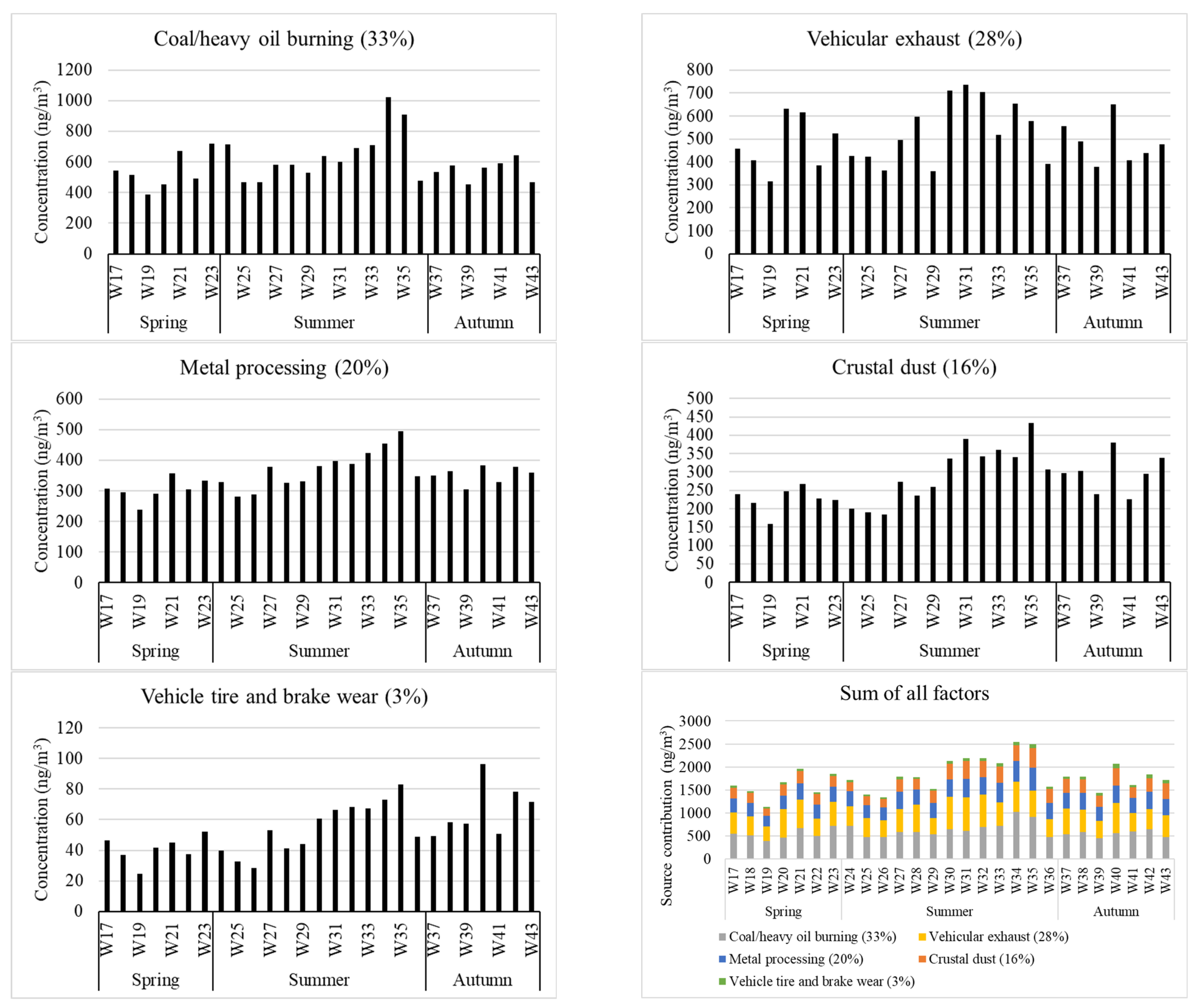
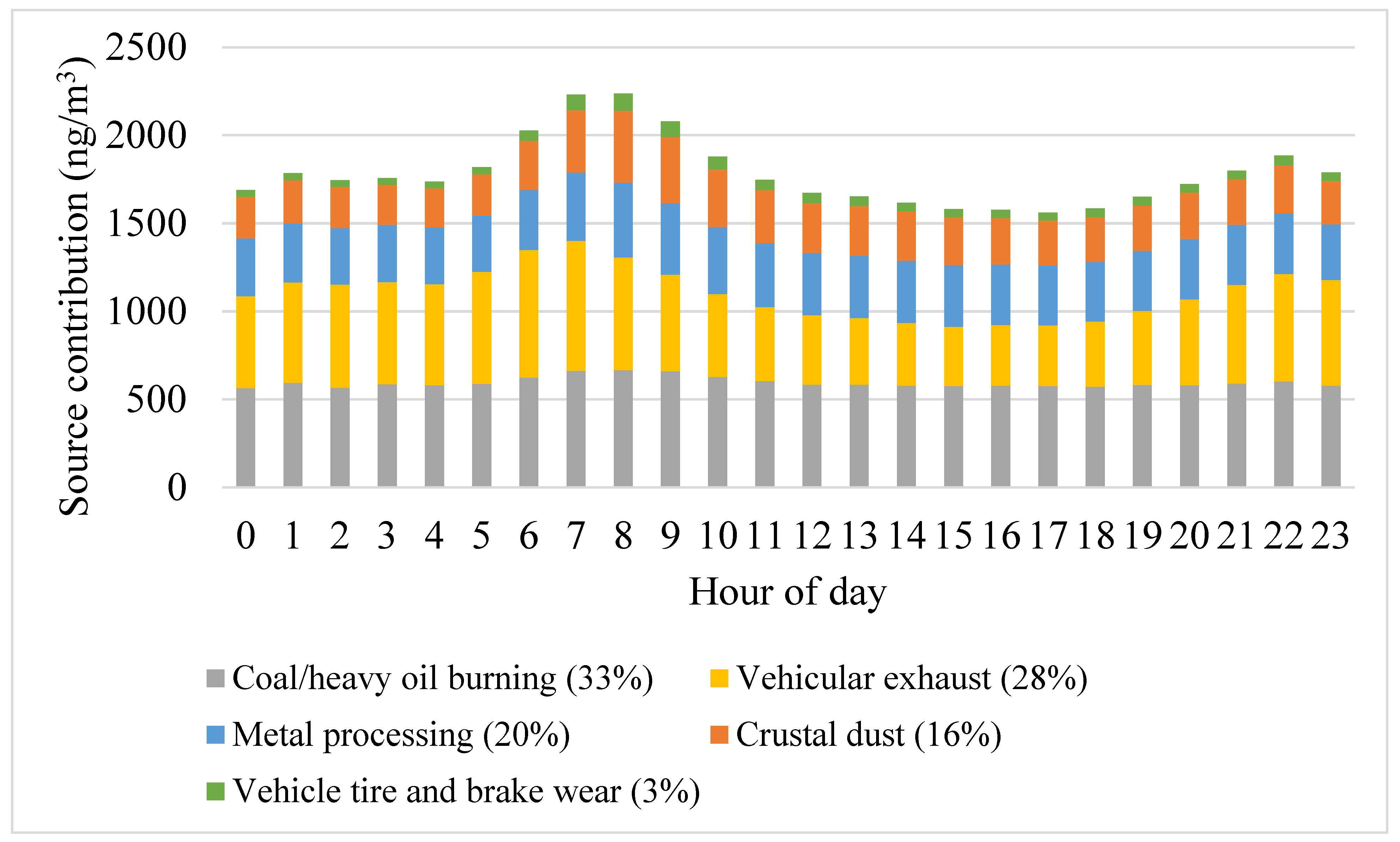
3.5. Source Apportionment of BC, BrCs, and PM2.5-Bound Elements

The predicted total PM2.5-bound element concentrations by the PMF model agreed well with the total measurements with a R2 value of 0.82 (Figure S8). In total, 9 out of the 27 species (BC, BrC1, BrC2, Ca, Mn, S, Si, Ti, and Zn) had high R2 values between predicted and observed concentrations that ranged from 0.59 to 0.88, with slopes ranging from 0.34 to 0.83. Four species (Br, Fe, Hg, and Se) had moderate R2 values between predicted and observed concentrations that ranged from 0.21 to 0.44, with slopes ranging from 0.11 to 0.43. Time series plots (not shown) indicate the predicted concentrations were underestimated. The PMF model was unable to accurately predict the concentrations of the remaining 14 PM2.5-bound elements (R2 < 0.14). More than 50% of the data points of these elements were below MDLs, except for Cu, K, Pb and Sr. These four elements showed extremely high concentrations on 3–5 July and 20 July 2021. The PMF model significantly underpredicted the concentrations of those species during the two episodes (Figure S9).
PMF modeling resulted in five source factors: (1) coal/heavy oil burning, (2) vehicular exhaust, (3) metal processing, (4) crustal dust, and (5) vehicle tire and brake wear. The highest contributing factor was coal/heavy oil burning, which accounted for 33% (Figure 2) of the PM2.5 elemental concentrations (BC, BrCs, and 24 other elements). This factor is dominated by high loadings of S (82%), Se (72%), Br (69%), and V (53%) and moderate loadings of Pb (43%) and K (27%) (Figure 2, Table S3). S and V are key markers of coal and heavy oil combustion sources, respectively [47,48]. In addition, the loadings of Br and Pb in this study are similar to the profiles of Br (50%) and Pb (50%) from coal combustion sources [49]. The loadings of Se and V in this study agreed with the profiles of Se (40%) and V (60%) from heavy oil combustion [50]. Although coal-fired power plants were eliminated in Ontario in 2014 [51], coal is still used to generate electricity in the neighboring US states of Michigan, Indiana, and Ohio. According to the US Energy Information Administration [52], coal provided the largest share of electricity generation in Michigan (32%) and Indiana (54%) in 2021, and the second largest share in Ohio (32%). In 2021, annual coal consumption in Michigan, Indiana, and Ohio was approximately 17, 29, and 22 million tons, respectively, which accounted for 3.6%, 6.1%, and 4.6% of total US coal consumption. Diurnal variation in source contributions of coal/heavy oil burning was small, with averaged hour-of-day contributions ranging from 570 ng/m3 at 0:00 to 670 ng/m3 at 8:00, suggesting coal/heavy oil burning is likely regional in nature.
The factor labelled as vehicular exhaust is the second-highest contributing factor (28%). This factor is characterized by high loadings of BrC1 (93%), BrC2 (90%), Sn (90%), As (75%), and BC (72%) and moderate loadings of Ba (31%), Cr (27%), Pb (27%), and Cu (20%) (Figure 2, Table S3). Diesel vehicle emission is one of the major sources of BC [53]. In addition, Pb and As are associated with exhaust emissions from diesel vehicles [54]. The loadings of Ba, Cu, and Pb in this study are similar to the profiles of vehicle exhaust from Chen et al. [55], i.e., Ba (40%), Cu (40%), and Pb (40%). As seen in Figure S10, the vehicular exhaust factor had elevated source contributions in the morning rush hours of 6:00–8:00 and a minimal contribution at 15:00, likely due to the maximum mixing heights in the afternoon that were followed by a gradual increase.
The next two factors, labelled as metal processing and crustal dust, contributed to 20% and 16% of the PM2.5-bounded elemental concentrations, respectively. The metal processing factor is characterized by high loadings of Hg (92%), Co (83%), Rb (77%), Ag (73%), Cd (71%), Si (56%), Ni (54%), Cu (44%), K (42%), and Sr (41%) (Figure 2 and Table S3). The loadings of Ag, Cd, Co, and Rb are similar to profiles reported in previous studies, i.e., iron ore and the steel industry from Hsu et al. [56] (Co: 80%) and metal processing from Wang et al. ([57] 75% Ag, 50% Cd, and 30% Rb). Diurnal variability in source contributions of metal processing was small (Figure S10), with averaged hour-of-day contributions ranging from 320 ng/m3 at 23:00 to 420 ng/m3 at 8:00, suggesting regional sources for the metal processing factor.
The crustal dust factor is characterized by high loadings of Ca (90%), Ti (59%), and Fe (55%) and moderate loadings of Mn (35%), Ba (31%), and Si (27%) (Figure 2, Table S3). Ca, Ti, Fe, and Si are tracers for crustal dust [31]. In addition, correlation coefficients among the four crustal elements are relatively high (0.4–0.8, p < 0.05, Table 2), suggesting a common source. Similar profiles of crustal dust were reported by Yu et al. [31], with loadings for Ca, Ti, Fe, Si, and Fe of ~80%, 70%, 40%, and 70%, respectively. The crustal dust factor had elevated factor contributions in the morning between 7:00 and 9:00 (Figure S10), suggesting resuspension of crustal dust by on-road vehicles.
The lowest contributing factor is vehicular tire and brake wear (3%). This factor is dominated by high loadings of Zn (79%) and Mn (58%) and moderate loadings of Fe (26%) (Figure 2 and Table S3). Zn is considered as a main tracer of the wear and abrasion of tires [38]. Farahani et al. [25] reported loading of 75% for Zn, 5% for Pb, and 5% for Ti in their profile of tire wear. The loadings of Mn and Fe are similar to the profiles of brake wear from Taghvaee et al. [58] (Mn (30%) and Fe (20%)). Correlation coefficients among the three elements (Zn, Mn, and Fe) are moderate (0.4–0.6, p < 0.05) (Table 2), suggesting they are likely emitted from the same source. The morning peak contributions of the vehicular tire and brake wear factor could be attributed to the morning rush hours and low mixing heights (Figure S10). The minimal contributions of this factor in the afternoon were likely due to maximum mixing heights, with contributions steadily increasing thereafter when mixing height was lower.
When combined, the three traffic-related factors (vehicular exhaust, crustal dust, and vehicle brake and tire wear) contributed to 47% of total PM2.5-bound elemental concentrations in Windsor. The coal/heavy oil burning and metal processing factors contributed to 33% and 20% of total concentrations, respectively. A source apportionment study in Toronto, Ontario, approximately 400 km northeast of Windsor, also identified local traffic-related sources and coal combustions that were related to regional sources between 2004 and 2017 [4]. The two factors contributed to 15% and 31% of total ambient PM2.5-bound species, respectively.
The weekly averages of hourly source contributions derived by the PMF model are shown in Figure 3. All five sources exhibited more elevated contributions in summer than in the other two seasons. Total source contributions were significantly higher in summer (1.9 µg/m3) compared to the other two seasons (1.5 µg/m3 in spring and 1.7 µg/m3 in fall, p < 0.05). This is not unexpected because most elements exhibited higher concentrations in summer than in spring and fall (Figure S11). The metal processing factor showed similar trends to the coal/heavy oil burning and vehicle tire and brake wear factors, with a high correlation coefficient of 0.81 and 0.82, respectively (p < 0.05, Table S4). The crustal dust and vehicle brake and tire wear factors also had similar trends (r = 0.88, p < 0.05, Table S4), suggesting road traffic as the major source.
Figure 4 depicts hour-of-day source contributions in Windsor during the study period. The diurnal trend in total contributions exhibits a bimodal pattern. A major peak was observed in the mornings from 7:00 to 8:00, when the morning commute is maximal and atmospheric mixing heights are low. A minor peak was observed in the evenings from 21:00 to 23:00 and could be partially due to the decreased atmospheric mixing heights [39]. In contrast, the total source contributions were low in the afternoon from 16:00 to 18:00 due to the maximum mixing heights. This pattern is consistent with the diurnal variations in most PM2.5-bound elements (Figure S4).
The three traffic-related sources, i.e., vehicular exhaust, crustal dust, and vehicle tire and brake wear, showed clear and similar diurnal variations. The contributions peaked in the morning between 6:00 and 9:00 owing to rush hour traffic and were low in the afternoon between 16:00 and 17:00 due to increased atmospheric mixing heights. The hour-of-day averaged contributions of vehicular exhaust ranged from 360 ng/m3 at 14:00 to 740 ng/m3 at 7:00. A similar diurnal pattern was also observed for crustal dust (223 ng/m3 at 4:00 to 409 ng/m3 at 8:00) and vehicle tire and brake wear (37 ng/m3 at 0:00 to 97 ng/m3 at 8:00). The large diurnal variations suggest that these three sources are mostly local emissions. In contrast, diurnal variability in the two industrial sources (the coal/heavy oil burning and metal processing factors) was small. The averaged hour-of-day contributions ranged from 570 ng/m3 at 0:00 to 670 ng/m3 at 8:00 for coal/heavy oil burning and ranged from 317 ng/m3 at 23:00 to 424 ng/m3 at 8:00 for metal processing. This suggests that these two industrial sources are of regional or transboundary origin.
Source contributions by wind direction are shown in Figure S12. Contributions of coal/heavy oil burning were higher when air masses came from the south than from the other three directions (720 ng/m3 in the south vs. 420–580 ng/m3 in the other three directions). This could be related to high S and Se emissions from power generation plants along the Ohio River valley (Figure S7). For metal processing, concentrations were higher when air masses were from the west where there are numerous metal processing facilities, including AK Steel Dearborn Works and Gerdau Special Steel North America in Michigan and ArcelorMittal Burns Harbor LLC and SDI Steel Dynamics Incorporated in Indiana. High values of the metal processing factor (75–95th percentile levels) were observed when air masses were from the west, which points to Zug Island as a possible source as it is owned by US Steel for iron and steelmaking and is approximately 3.5 km west of the Windsor West monitoring station (Figure 1). The island released 3.3 kg of Pb, 1.5 kg of Ni, 0.8 kg of Cd, and 0.06 kg of Co from US Steel’s Great Lakes Works in 2017 [19].
The three traffic-related sources (i.e., vehicular exhaust, crustal dust, and vehicle tire and brake wear) showed higher source contributions when air masses were from the west and southwest (Figure S12). The sources of those three factors were likely local due to heavy traffic within a few kilometers of the monitoring station due to the presence of Huron Church Road and Ambassador Bridge, the busiest international transportation corridor in North America, and intensive construction work for the Gordie Howe International Bridge, which is located 2 km to the west of the monitoring station.

4. Conclusions

PM2.5, BC, and PM2.5-bound elements were continuously monitored from April to October 2021 during the MOOSE field campaign. The hourly data were used to assess levels and temporal variations in trace elements in Windsor, especially diurnal patterns. The pollution roses and PMF analysis were further used to identify emission sources and their relative contributions. The concentrations of trace elements in Windsor in 2021 were generally comparable to the measurements between 2017 and 2019 in Windsor, Hamilton, which were impacted by industrial emissions, and at the HWY 401 station, which is close to road traffic; however, they were higher than other stations in Ontario (i.e., Sudbury, Toronto North, Ottawa Downtown, and Simcoe). Ontario’s 24 h AAQC for the PM2.5 fraction were not exceeded for any elements, except for one Fe exceedance likely related to industrial emissions. Correlation analyses further identified the pollutants likely released from common emission sources, i.e., BC and BrCs from fossil fuel burning (r ranging from 0.46 to 0.84, p < 0.05) and Fe, Ca, Mn, Si, Ti, and Zn from crustal dust (r ranging from 0.54 to 0.79, p < 0.05).
Diurnal variations in air pollutants were assessed to reveal the impact of local emissions that are governed by human and industrial activities and local meteorology. PM2.5, BC, and most of the PM2.5-bound elements showed a clear diurnal pattern, i.e., elevated concentrations in the morning rush hours between 6:00 and 9:00 and valleyed concentrations in the late afternoon between 15:00 and 17:00 when mixing heights are maximal or in the early morning between 3:00 and 4:00 when human activity is minimal. The results indicate that diurnal variation in the air pollutants in Windsor was mainly attributed to evolution of the atmospheric boundary layer and local anthropogenic activities. Sulfur showed a unique diurnal pattern with elevated concentrations in the afternoon between 13:00 and 16:00, a time when sulphate production through photochemical reactions is enhanced due to increased ambient temperatures.
The PMF model successfully apportioned the ambient BC, BrCs, and PM2.5-bound element concentrations in Windsor into five sources: (1) coal/heavy oil burning (33% of total PM2.5-bound elemental concentration), (2) vehicular exhaust (28%), (3) metal processing (20%), (4) crustal dust (16%), and (5) vehicle tire and brake wear (3%). Overall, the three traffic-related sources, i.e., vehicular exhaust, crustal dust, and vehicle tire and brake wear, were primarily from local sources (heavy traffic on Huron Church Road and Ambassador Bridge and intensive construction work for the Gordie Howe International Bridge within several kilometers of the station). Coal/heavy oil burning and metal processing may originate from regional or transboundary sources, as supported by weak diurnal variability and elevated industrial emissions in neighboring states. When combined, the three local traffic-related sources (vehicular exhaust, crustal dust, and vehicle brake and tire wear) contributed to 47% of total measured PM2.5-bound elemental concentrations in Windsor during the study period. The two regional/transboundary sources, i.e., coal/heavy oil burning and metal processing, contributed to the remaining 53%. Control measures should be developed to reduce both local traffic emissions and regional/transboundary industrial emissions in order to mitigate the levels of PM2.5-bound elements in Windsor.
In this study, pollution roses and emission inventories were used in conjunction with diurnal variations to assess the impact of local and regional/transboundary sources. However, long-range transport could be further studied with other approaches, such as the Hybrid Single-Particle Lagrangian Integrated Trajectory model (HYSPLIT) [59] and the potential source contribution function (PSCF) [60]. The total PM2.5-bound element concentrations predicted by the PMF model were in good agreement with the total measured values, with a R2 value of 0.82. However, the PMF model underpredicted the concentrations of elements with over 50% of data points below MDLs or those showing elevated concentrations during the two episodic events. The measurements below MDLs were included as is in the current PMF analysis along with hourly BC and BrC data. Future study is warranted to carry out enrichment factor analysis [61] to determine the origin of trace elements and to evaluate how source apportionment by PMF analysis for PM2.5-bound elements is impacted by the treatment of data below MDLs, the elevated concentrations in the two episodic events, and the inclusion/exclusion of black carbon and brown carbon data.

Supplementary Materials

The following supporting information can be downloaded at: https://www.mdpi.com/article/10.3390/atmos14020374/s1, Figure S1: IM and IS vs. number of factors; Figure S2: Q (Robust) and Q (True) vs. number of factors; Figure S3: Relative contributions of black carbon (BC) and brown carbons (BrC1 and BrC2) and 24 PM2.5-bound elements. The total contributions by the 18 elements (Cu, Mn, Cd, Ti, Pb, Br, Ba, Ag, Sr, Se, Hg, Ni, V, Cr, As, Sn, Rb, and Co) was 1.7%; Figure S4: Diurnal variations of PM2.5, BC, brown carbons (BrC1 and BrC2), and PM2.5-bound element concentrations. The dots indicate the mean values and the error bars represent the 95% confidence intervals; Figure S5: Diurnal variations of wind speed (left) and ambient temperature (right). The dots indicate the mean values and the error bars represent the 95% confidence intervals; Figure S6: Pollution roses of PM2.5 mass, black carbon, brown carbons, and 14 selected PM2.5-bound elements; Figure S7: NPRI and NEI emission maps of Hg, Mn, Pb, PM2.5, Se, and SO2 in Ontario in 2020 and surrounding nine US states in 2017; Figure S8: Scatter plots of hourly total observed concentrations vs. hourly total predicted concentration. The two episodes are labelled in orange and green, respectively; Figure S9: Time-series of hourly observed concentrations vs. predicted concentration for Cu, K, Pb and Sr; Figure S10: Diurnal variations of source contributions (ng/m3) of each source in Windsor. The dots indicate the mean values and the error bars represent the 95% confidence intervals; Figure S11: Seasonal variations of PM2.5, BC, brown carbons (BrC1 and BrC2), and PM2.5-bound element concentrations in Windsor during the study period. The dots indicate the mean values and the error bars represent the 95% confidence intervals; Figure S12: Pollution roses of source contributions in Windsor, Canada. Table S1: Average concentrations of PM2.5-bound elements measured by the Xact 625 analyzer from April to October 2021 at Windsor West, and by the Dichot method as described in Dabek-Zlotorzynska et al., [8] in 2017-2019 at seven 7 stations in Ontario. Site classification and source influences were obtained from Environment and Climate Change Canada website [9]; Table S2: Statistics of 24-h concentrations for 14 PM2.5-bound elements with ≥50% MDL in this study and Ontario’s Ambient Air Quality Criteria (AAQC) [32]; Table S3: Factor profiles (% of species mass concentrations being assigned to that factor) for black carbon (BC) and brown carbons (BrC1 and BrC2), and PM2.5-bound elements in Windsor during April–October 2021. Bold values are percentages ≥40%; Table S4: Pearson correlation coefficients of weekly averaged contributions among the five factors identified by the PMF.

Author Contributions

Conceptualization, methodology, and supervision, Y.S. and X.X.; data curation, J.D., M.N. and A.M.; formal analysis and visualization, T.Z.; writing—original draft preparation, T.Z. and Y.S.; writing—review and editing, Y.S. and X.X.; funding acquisition, Y.S. and X.X. All authors have read and agreed to the published version of the manuscript.

Funding

This research was funded by Environment and Climate Change Canada, the Natural Sciences and Engineering Research Council of Canada, and University of Windsor’s Ignite Program.

Institutional Review Board Statement

Not applicable.

Informed Consent Statement

Not applicable.

Data Availability Statement

The following datasets are publicly available and can be downloaded from government websites. Annual air emission data in Ontario, Canada, in 2020 can be found at: https://pollution-waste.canada.ca/national-release-inventory/ accessed on 10 February 2023. Annual air emission data in the nine US states (Wisconsin, Illinois, Michigan, Indiana, Kentucky, Ohio, West Virginia, Pennsylvania, and New York) in 2017 can be found at: https://www.epa.gov/air-emissions-inventories/2017-national-emissions-inventory-nei-data accessed on 10 February 2023. Concentrations of twenty-four-hour integrated PM2.5-bound elements can be found at https://data-donnees.ec.gc.ca/data/air/monitor/national-air-pollution-surveillance-naps-program/Data-Donnees/?lang=en accessed on 10 February 2023. Hourly concentrations of PM2.5, black carbons, and PM2.5-bound elements and meteorological data between April and October 2021 are available upon request from the corresponding author or at the repository for the MOOSE study https://www-air.larc.nasa.gov/missions/moose/index.html accessed on 10 February 2023.

Acknowledgments

Environment and Climate Change Canada’s National Air Pollution Surveillance program is acknowledged for providing the air monitoring instrumentation. The authors thank Lindsay Miller-Branovackiat and Donald Bourne at the University of Windsor for their editorial assistance, Carina Luo at the University of Windsor for creating the emission density maps, and Chris Charron at the Ontario Ministry of the Environment, Conservation and Parks for his support with participation in the MOOSE study.

Conflicts of Interest

The authors declare no conflict of interest.

References

  1. Tucker, W. An overview of PM2.5 sources and control strategies. Fuel Process. Technol. 2000, 65–66, 379–392. [Google Scholar] [CrossRef]
  2. Sofowote, U.M.; Su, Y.; Dabek-Zlotorzynska, E.; Rastogi, A.K.; Brook, J.; Hopke, P.K. Sources and temporal variations of constrained PMF factors obtained from multiple-year receptor modeling of ambient PM2.5 data from five speciation sites in Ontario, Canada. Atmos. Environ. 2015, 108, 140–150. [Google Scholar] [CrossRef]
  3. Healy, R.; Sofowote, U.; Su, Y.; Debosz, J.; Noble, M.; Jeong, C.-H.; Wang, J.; Hilker, N.; Evans, G.; Doerksen, G.; et al. Ambient measurements and source apportionment of fossil fuel and biomass burning black carbon in Ontario. Atmos. Environ. 2017, 161, 34–47. [Google Scholar] [CrossRef]
  4. Jeong, C.-H.; Traub, A.; Huang, A.; Hilker, N.; Wang, J.M.; Herod, D.; Dabek-Zlotorzynska, E.; Celo, V.; Evans, G.J. Long-term analysis of PM2.5 from 2004 to 2017 in Toronto: Composition, sources, and oxidative potential. Environ. Pollut. 2020, 263, 114652. [Google Scholar] [CrossRef]
  5. Loomis, D.; Grosse, Y.; Lauby-Secretan, B.; El Ghissassi, F.; Bouvard, V.; Benbrahim-Tallaa, L.; Baan, R.; Mattock, H.; Straif, K.; International Agency for Research on Cancer Monograph Working Group IARC. The carcinogenicity of outdoor air pollution. Lancet Oncol. 2013, 14, 1262. [Google Scholar] [CrossRef]
  6. Health Canada (HC). Canadian Health Science Assessment for Fine Particulate Matter (PM2.5); Health Canada: Ottawa, ON, Canada, 2022; ISBN 978-0-660-41742-4.
  7. Ontario Ministry of the Environment, Conservation and Parks (MECP). Air Quality in Ontario 2019 Report. 2020. Available online: https://www.ontario.ca/document/air-quality-ontario-2019-report (accessed on 14 October 2022).
  8. Dabek-Zlotorzynska, E.; Dann, T.F.; Martinelango, P.K.; Celo, V.; Brook, J.R.; Mathieu, D.; Ding, L.; Austin, C.C. Canadian National Air Pollution Surveillance (NAPS) PM2.5 speciation program: Methodology and PM2.5 chemical composition for the years 2003–2008. Atmos. Environ. 2011, 45, 673–686. [Google Scholar] [CrossRef]
  9. Environment and Climate Change Canada (ECCC). National Air Pollution Surveillance (NAPS) Program. 2022. Available online: https://data-donnees.ec.gc.ca/data/air/monitor/national-air-pollution-surveillance-naps-program/ProgramInformation-InformationProgramme/?lang=en. (accessed on 3 February 2022).
  10. Lyamani, H.; Olmo, F.J.; Alados-Arboledas, L. Physical and optical properties of aerosols over an urban location in Spain: Seasonal and diurnal variability. Atmos. Meas. Tech. 2010, 10, 239–254. [Google Scholar] [CrossRef]
  11. Sofowote, U.M.; Healy, R.M.; Su, Y.; Debosz, J.; Noble, M.; Munoz, A.; Jeong, C.-H.; Wang, J.M.; Hilker, N.; Evans, G.J.; et al. Understanding the PM2.5 imbalance between a far and near-road location: Results of high temporal frequency source apportionment and parameterization of black carbon. Atmos. Environ. 2018, 173, 277–288. [Google Scholar] [CrossRef]
  12. Su, Y.; Sofowote, U.; Debosz, J.; White, L.; Munoz, A. Multi-year continuous PM2.5 measurements with the Federal Equivalent Method SHARP 5030 and comparisons to filter based and TEOM measurements in Ontario, Canada. Atmosphere 2018, 9, 191. [Google Scholar] [CrossRef]
  13. United States Environmental Protection Agency (US EPA). EPA Positive Matrix Factorization (PMF) 5.0 Fundamentals and User Guide. 2014. Available online: https://www.epa.gov/sites/default/files/2015-02/documents/pmf_5.0_user_guide.pdf (accessed on 14 October 2022).
  14. United States Department of Transpiration (USDT). Ambassador Bridge Crossing Summary. 2020. Available online: https://ops.fhwa.dot.gov/freight/freight_analysis/ambass_brdg/ambass_brdge_ovrvw.htm (accessed on 14 October 2022).
  15. Buffalo and Fort Erie Public Bridge Authority (BFEPBA), 2018 Traffic Statistics Issued by the Bridge and Tunnel Operators Association (BTOA). 2019. Available online: https://www.peacebridge.com/index.php/media-room/press-releases-advisories/381-btoa-2018-stats (accessed on 14 October 2022).
  16. United States Environmental Protection Agency (US EPA). United States Files Complaint Against EES Coke in River Rouge, Michigan, for Clean Air Act Violations. 2022. Available online: https://www.epa.gov/newsreleases/united-states-files-complaint-against-ees-coke-river-rouge-michigan-clean-air-act (accessed on 14 October 2022).
  17. Jin, Q.; Liu, Y.; Feng, M.; Huang, C. High-resolution temporal metallic elements in PM2.5 in Chengdu, Southwest China: Variations, extreme events, and effects of meteorological parameters. Air Qual. Atmosphere Health 2021, 14, 1893–1909. [Google Scholar] [CrossRef]
  18. National Pollutant Release Inventory (NPRI). National Pollutant Release Inventory Data Search. 2022. Available online: https://pollution-waste.canada.ca/national-release-inventory/ (accessed on 14 October 2022).
  19. National Emissions Inventory (NEI). 2017 National Emissions Inventory (NEI) Data. 2017. Available online: https://www.epa.gov/air-emissions-inventories/2017-national-emissions-inventory-nei-data (accessed on 14 October 2022).
  20. Environmental Systems Research Institute (ESRI). Heat Map Symbology. 2023. Available online: https://pro.arcgis.com/en/pro-app/latest/help/mapping/layer-properties/heat-map.htm (accessed on 2 February 2022).
  21. Hedberg, E.; Gidhagen, L.; Johansson, C. Source contributions to PM10 and arsenic concentrations in Central Chile using positive matrix factorization. Atmos. Environ. 2005, 39, 549–561. [Google Scholar] [CrossRef]
  22. Pekey, H.; Karakaş, D.; Bakoglu, M. Source apportionment of trace metals in surface waters of a polluted stream using multivariate statistical analyses. Mar. Pollut. Bull. 2004, 49, 809–818. [Google Scholar] [CrossRef] [PubMed]
  23. Lee, E.; Chan, C.K.; Paatero, P. Application of positive matrix factorization in source apportionment of particulate pollutants in Hong Kong. Atmos. Environ. 1999, 33, 3201–3212. [Google Scholar] [CrossRef]
  24. Shin, S.M.; Kim, J.Y.; Lee, J.Y.; Kim, D.S.; Kim, Y.P. Enhancement of modeling performance by including organic markers to the PMF modeling for the PM2.5 at Seoul. Air Qual. Atmos. Health 2022, 15, 91–104. [Google Scholar]
  25. Farahani, V.J.; Soleimanian, E.; Pirhadi, M.; Sioutas, C. Long-term trends in concentrations and sources of PM2.5-bound metals and elements in central Los Angeles. Atmos. Environ. 2021, 253, 118361. [Google Scholar] [CrossRef]
  26. Peralta, O.; Ortínez-Alvarez, A.; Basaldud, R.; Santiago, N.; Alvarez-Ospina, H.; de la Cruz, K.; Barrera, V.; de la Luz Espinosa, M.; Saavedra, I.; Castro, T.; et al. Atmospheric black carbon concentrations in Mexico. Atmos. Res. 2019, 230, 104626. [Google Scholar] [CrossRef]
  27. Anastasopolos, A.T.; Hopke, P.K.; Sofowote, U.M.; Zhang, J.J.; Johnson, M. Local and regional sources of urban ambient PM2.5 exposures in Calgary, Canada. Atmos. Environ. 2022, 290, 119383. [Google Scholar] [CrossRef]
  28. Nayebare, S.R.; Aburizaiza, O.S.; Siddique, A.; Carpenter, D.O.; Hussain, M.M.; Zeb, J.; Aburiziza, A.J.; Khwaja, H.A. Ambient air quality in the holy city of Makkah: A source apportionment with elemental enrichment factors (EFs) and factor analysis (PMF). Environ. Pollut. 2018, 243, 1791–1801. [Google Scholar] [CrossRef]
  29. Al Mamun, A.; Celo, V.; Dabek-Zlotorzynska, E.; Charland, J.-P.; Cheng, I.; Zhang, L. Characterization and source apportionment of airborne particulate elements in the Athabasca oil sands region. Sci. Total. Environ. 2021, 788, 147748. [Google Scholar] [CrossRef]
  30. Liu, Y.; Yang, Z.; Liu, Q.; Qi, X.; Qu, J.; Zhang, S.; Wang, X.; Jia, K.; Zhu, M. Study on chemical components and sources of PM2.5 during heavy air pollution periods at a suburban site in Beijing of China. Atmos. Pollut. Res. 2021, 12, 188–199. [Google Scholar] [CrossRef]
  31. Yu, Y.; He, S.; Wu, X.; Zhang, C.; Yao, Y.; Liao, H.; Wang, Q.; Xie, M. PM2.5 elements at an urban site in Yangtze River Delta, China: High time-resolved measurement and the application in source apportionment. Environ. Pollut. 2019, 253, 1089–1099. [Google Scholar] [CrossRef] [PubMed]
  32. Ontario Ministry of the Environment, Conservation and Parks (MECP). Ontario’s Ambient Air Quality Criteria. 2019. Available online: https://www.ontario.ca/page/ontarios-ambient-air-quality-criteria (accessed on 14 October 2022).
  33. Morawska, L.; Thomas, S.; Bofinger, N.; Wainwright, D.; Neale, D. Comprehensive characterization of aerosols in a subtropical urban atmosphere: Particle size distribution and correlation with gaseous pollutants. Atmos. Environ. 1998, 32, 2467–2478. [Google Scholar] [CrossRef]
  34. Saeedi, M.; Li, L.Y.; Salmanzadeh, M. Heavy metals and polycyclic aromatic hydrocarbons: Pollution and ecological risk assessment in street dust of Tehran. J. Hazard. Mater. 2012, 227, 9–17. [Google Scholar] [CrossRef]
  35. Cyrys, J.; Stölzel, M.; Heinrich, J.; Kreyling, W.G.; Menzel, N.; Wittmaack, K.; Tuch, T.; Wichmann, H.E. Elemental composition and sources of fine and ultrafine ambient particles in Erfurt, Germany. Sci. Total Environ. 2003, 305, 143–156. [Google Scholar] [CrossRef] [PubMed]
  36. Ni, M.; Huang, J.; Lu, S.; Li, X.; Yan, J.; Cen, K. A review on black carbon emissions, worldwide and in China. Chemosphere 2014, 107, 83–93. [Google Scholar] [CrossRef] [PubMed]
  37. Kotchenruther, R.A. The effects of marine vessel fuel sulfur regulations on ambient PM2.5 at coastal and near coastal monitoring sites in the U.S. Atmos. Environ. 2017, 151, 52–61. [Google Scholar] [CrossRef]
  38. Harrison, R.M.; Jones, A.M.; Gietl, J.; Yin, J.; Green, D.C. Estimation of the Contributions of Brake Dust, Tire Wear, and Resuspension to Nonexhaust Traffic Particles Derived from Atmospheric Measurements. Environ. Sci. Technol. 2012, 46, 6523–6529. [Google Scholar] [CrossRef]
  39. Yassin, M.F.; Al-Shatti, L.A.; Al Rashidi, M.S. Assessment of the atmospheric mixing layer height and its effects on pollutant dispersion. Environ. Monit. Assess. 2018, 190, 372. [Google Scholar] [CrossRef]
  40. Retama, A.; Baumgardner, D.; Raga, G.B.; McMeeking, G.R.; Walker, J.W. Seasonal and diurnal trends in black carbon properties and co-pollutants in Mexico City. Atmos. Meas. Tech. 2015, 15, 9693–9709. [Google Scholar] [CrossRef]
  41. Chen, R.; Jia, B.; Tian, Y.; Feng, Y. Source-specific health risk assessment of PM2.5-bound heavy metals based on high time-resolved measurement in a Chinese megacity: Insights into seasonal and diurnal variations. Ecotoxicol. Environ. Saf. 2021, 216, 112167. [Google Scholar] [CrossRef]
  42. Hasheminassab, S.; Sowlat, M.H.; Pakbin, P.; Katzenstein, A.; Low, J.; Polidori, A. High time-resolution and time-integrated measurements of particulate metals and elements in an environmental justice community within the Los Angeles Basin: Spatio-temporal trends and source apportionment. Atmos. Environ. X 2020, 7, 100089. [Google Scholar] [CrossRef]
  43. Zhao, S.; Tian, H.; Luo, L.; Liu, H.; Wu, B.; Liu, S.; Bai, X.; Liu, W.; Liu, X.; Wu, Y.; et al. Temporal variation characteristics and source apportionment of metal elements in PM2.5 in urban Beijing during 2018–2019. Environ. Pollut. 2021, 268, 115856. [Google Scholar] [CrossRef]
  44. Marcazzan, G.M.; Vaccaro, S.; Valli, G.; Vecchi, R. Characterisation of PM10 and PM2.5 particulate matter in the ambient air of Milan (Italy). Atmos. Environ. 2001, 35, 4639–4650. [Google Scholar] [CrossRef]
  45. Zhang, T.; Xu, X.; Su, Y. Impacts of Regional Transport and Meteorology on Ground-Level Ozone in Windsor, Canada. Atmosphere 2020, 11, 1111. [Google Scholar] [CrossRef]
  46. McGuire, M.L.; Chang, R.Y.-W.; Slowik, J.G.; Jeong, C.-H.; Healy, R.M.; Lu, G.; Mihele, C.; Abbatt, J.P.D.; Brook, J.R.; Evans, G.J. Enhancing non-refractory aerosol apportionment from an urban industrial site through receptor modeling of complete high time-resolution aerosol mass spectra. Atmos. Meas. Tech. 2014, 14, 8017–8042. [Google Scholar] [CrossRef]
  47. Chou, C.-L. Sulfur in coals: A review of geochemistry and origins. Int. J. Coal Geol. 2012, 100, 1–13. [Google Scholar] [CrossRef]
  48. Hao, Y.; Meng, X.; Yu, X.; Lei, M.; Li, W.; Shi, F.; Yang, W.; Zhang, S.; Xie, S. Characteristics of trace elements in PM2.5 and PM10 of Chifeng, northeast China: Insights into spatiotemporal variations and sources. Atmos. Res. 2018, 213, 550–561. [Google Scholar] [CrossRef]
  49. Chi, R.; Li, H.; Wang, Q.; Zhai, Q.; Wang, D.; Wu, M.; Liu, Q.; Wu, S.; Ma, Q.; Deng, F.; et al. Association of emergency room visits for respiratory diseases with sources of ambient PM2.5. J. Environ. Sci. 2019, 86, 154–163. [Google Scholar] [CrossRef]
  50. Sugiyama, T.; Shimada, K.; Miura, K.; Lin, N.-H.; Kim, Y.P.; Chan, C.K.; Takami, A.; Hatakeyama, S. Measurement of Ambient PAHs in Kumamoto: Differentiating Local and Transboundary Air Pollution. Aerosol Air Qual. Res. 2017, 17, 3106–3118. [Google Scholar] [CrossRef]
  51. Ontario Environment and Energy (OEE). The End of Coal. 2021. Available online: https://www.ontario.ca/page/end-coal (accessed on 14 October 2022).
  52. United States Energy Information Administration (USEIA). Michigan State Energy Profile. 2022. Available online: https://www.eia.gov/state/print.php?sid=MI#:~:text=Michigan%20Quick%20Facts&text=In%202021%2C%20coal%20provided%20the,three%2Dfifths%20of%20that%20power (accessed on 14 October 2022).
  53. Wang, H.; Zhang, L.; Cheng, I.; Yao, X.; Dabek-Zlotorzynska, E. Spatiotemporal trends of PM2.5 and its major chemical components at urban sites in Canada. J. Environ. Sci. 2021, 103, 1–11. [Google Scholar] [CrossRef]
  54. Jaiprakash; Habib, G. Chemical and optical properties of PM2.5 from on-road operation of light duty vehicles in Delhi city. Sci. Total. Environ. 2017, 586, 900–916. [Google Scholar] [CrossRef] [PubMed]
  55. Chen, R.; Zhao, Y.; Tian, Y.; Feng, X.; Feng, Y. Sources and uncertainties of health risks for PM2.5-bound heavy metals based on synchronous online and offline filter-based measurements in a Chinese megacity. Environ. Int. 2022, 164, 107236. [Google Scholar] [CrossRef]
  56. Hsu, C.-Y.; Chiang, H.-C.; Chen, M.-J.; Chuang, C.-Y.; Tsen, C.-M.; Fang, G.-C.; Tsai, Y.-I.; Chen, N.-T.; Lin, T.-Y.; Lin, S.-L.; et al. Ambient PM2.5 in the residential area near industrial complexes: Spatiotemporal variation, source apportionment, and health impact. Sci. Total. Environ. 2017, 590, 204–214. [Google Scholar] [CrossRef] [PubMed]
  57. Wang, J.; Jiang, H.; Jiang, H.; Mo, Y.; Geng, X.; Li, J.; Mao, S.; Bualert, S.; Ma, S.; Li, J.; et al. Source apportionment of water-soluble oxidative potential in ambient total suspended particulate from Bangkok: Biomass burning versus fossil fuel combustion. Atmos. Environ. 2020, 235, 117624. [Google Scholar] [CrossRef]
  58. Taghvaee, S.; Sowlat, M.H.; Mousavi, A.; Hassanvand, M.S.; Yunesian, M.; Naddafi, K.; Sioutas, C. Source apportionment of ambient PM2.5 in two locations in central Tehran using the Positive Matrix Factorization (PMF) model. Sci. Total. Environ. 2018, 628, 672–686. [Google Scholar] [CrossRef]
  59. Stein, A.F.; Draxler, R.R.; Rolph, G.D.; Stunder, B.J.B.; Cohen, M.D.; Ngan, F. NOAA’s HYSPLIT Atmospheric Transport and Dispersion Modeling System. Bull. Am. Meteorol. Soc. 2015, 96, 2059–2077. [Google Scholar] [CrossRef]
  60. Ashbaugh, L.L.; Malm, W.C.; Sadeh, W.Z. A residence time probability analysis of sulfur concentrations at grand Canyon National Park. Atmos. Environ. 1985, 19, 1263–1270. [Google Scholar] [CrossRef]
  61. Reimann, C.; Caritat, P.D. Intrinsic flaws of element enrichment factors (EFs) in environmental geochemistry. Environ. Sci. Technol. 2000, 34, 5084–5091. [Google Scholar] [CrossRef]
Figure 1. Location of the Windsor West air monitoring station in Ontario, Canada.
Atmosphere 14 00374 g001
Figure 2. Profiles of five factors identified from the PMF model for BC, BrCs, and PM2.5-bound elements in Windsor during the study period. Percentage of species (diamond symbol) as the secondary Y-axis is the percentage of species mass concentrations being assigned to that factor. Percentages in the subtitles are average source contributions.
Atmosphere 14 00374 g002
Figure 3. Weekly averaged source contributions to ambient PM2.5-bound elements. Percentages in the bracket are averaged source contributions. Week 17 started on 20 April 2021 and W43 started on 17 October 2021. Spring is from April to May, summer is from June to August, and fall is from September to October.
Atmosphere 14 00374 g003
Figure 4. Diurnal variations in source contributions to ambient PM2.5-bound elements.
Atmosphere 14 00374 g004
Table 1. Statistics of hourly concentrations for PM2.5, BC and BrCs (µg/m3), and PM2.5-bound elements (ng/m3) between April and October 2021 (N = 4362).
SpeciesMeanStd DevMinMedianMaxMDLMissing (%)<MDL (%)Flags (%)Valid (%)
PM2.59.16.108.0480.51.94.12.691
BC0.60.40.0130.54.80.0051.94.12.691
BrC1 *0.10.10.0010.042.1NA2.6140.184
BrC2 *0.10.10.0010.061.6NA2.60.80.197
Ag2.71.502.3144.3311734.211
As0.21.100330.1111724.213
Ba2.91301.03700.9511404.245
Br3.22.602.7490.18111.34.283
Ca8912005216000.9110.54.284
Cd4.42.00.124.2175.7511664.219
Co0.030.10060.3211834.21.1
Cr0.33.000.061100.2911674.218
Cu4.8101.53.22560.271104.284
Fe1202500.366575000.76110.14.284
Hg0.60.600.45100.1911244.260
K120260338370002.371104.284
Mn4.69.301.81500.28113.64.281
Ni0.51.700.27410.2311354.249
Pb3.98.60.253.03400.221104.284
Rb0.20.200.162.90.3411704.214
S6005408.1440410061104.284
Se0.71.100.35200.1411184.266
Si410220473603300201104.284
Sn0.24.4001407.4611844.20.4
Sr1.66.70.10.861800.45117.84.277
Ti4.14.202.9550.38111.54.283
V0.51.200.13310.2911554.229
Zn26560.03108400.23110.34.284
Note: Missing (%) + <MDL (%) + Flags (%) + Valid (%) = 100%. * BrC1 and BrC2 concentrations were calculated.
Table 2. Correlation coefficients among PM2.5, BC, BrCs, and PM2.5-bound elements. Italic values indicate p-value ≥0.05.
PM2.5BCBrC1 BrC2 Br Ca Cu Fe Hg K Mn Pb S Se Si Sr Ti
BC0.59
BrC1 0.360.56
BrC2 0.460.840.82
Br 0.470.400.290.33
Ca 0.160.370.180.310.16
Cu 0.290.340.350.370.220.16
Fe 0.190.390.480.460.290.470.37
Hg −0.030.050.130.090.010.120.090.34
K 0.320.250.230.260.160.070.920.080.01
Mn 0.150.390.300.390.150.480.270.500.160.14
Pb 0.140.260.210.270.190.170.230.320.060.130.16
S 0.510.240.010.050.470.070.150.060.030.180.060.11
Se 0.240.140.030.060.360.080.050.060.010.050.060.050.33
Si 0.210.230.100.160.180.640.130.360.080.110.280.110.220.11
Sr 0.250.200.190.210.110.070.900.070.010.980.120.110.140.040.08
Ti 0.300.390.210.320.250.620.450.380.040.440.410.160.240.170.800.41
Zn 0.090.280.190.260.140.280.180.350.130.070.640.140.090.130.170.060.20
Disclaimer/Publisher’s Note: The statements, opinions and data contained in all publications are solely those of the individual author(s) and contributor(s) and not of MDPI and/or the editor(s). MDPI and/or the editor(s) disclaim responsibility for any injury to people or property resulting from any ideas, methods, instructions or products referred to in the content.

