Abstract
Global and urban-induced local warming lead to increasing heat risk in cities. The rapid increase in urban population, weak infrastructure, poverty, as well as an ageing population, make the risk more acute in developing cities. However, heat risk is not uniformly distributed and a detailed exploration of the link between urban characteristics and local variations in heat risk is needed to aid targeted mitigation. In this paper, we demonstrate a fine-grained heat risk map using existing data combined with expert opinion in a humid tropical city (Colombo, Sri Lanka) with the objective of highlighting the relative heat risk as a function of physical and socioeconomic conditions across the city. We then simulate the effects of shading and greening on the ‘high’ heat risk areas, and greening on the ‘low’ heat risk areas, to show that a combined approach will be needed to reduce risk at ‘high’ risk areas. In ‘low’ risk areas, maintaining the green cover is crucial to heat risk reduction. The paper, thus, establishes a protocol for detailed heat risk mapping with existing data and points to the differing importance of shading and greening in different parts of the city, thus, showing where, and to what extent, mitigation actions could be beneficial.
1. Introduction
Urban heat risk is increasing across the world as a consequence of global climate change and the UHI effect. Heat risk in developing cities is disproportionately high due to weak infrastructure, poverty, as well as an ageing population [1]. As acknowledged by the 6th Assessment Report of the First Working Group of IPCC [2], the temperature signal of urbanisation itself may be negligible at the global scale, but the relative share of urban warming (as denoted by the UHI effect) as a percentage of total warming in cities is significant: U.S. (14–21%); Europe (16%) and China (33%) [3]. It could be even higher in warm climate cities (from 50% up to 76% [2]). Additionally, there is evidence that UHI intensities increase during heatwaves in coastal cities [4], although the night-time situation may even be reversed [5].
There is strong evidence that the interactions between changing urban form, exposure due to urbanisation, and vulnerability due to changing demographics, can exacerbate heat risks and losses for cities and settlements [6]. This highlights the need to uncover local variations in heat risk, since intra-urban characteristics of the risk could aid targeted mitigation [4]. As defined by the IPCC [7], ‘Climate risk’ is a function of ‘hazard’, ‘exposure’ and ‘vulnerability’. Thus, ‘heat risk’ is a function of high/extreme temperatures (hazard), which are mediated by the built environment, shading, greenery, and other built infrastructure (exposure). This is further influenced by socioeconomic characteristics of population (including age and health [8]). Detailed approaches to heat risk mapping are needed to understand the spatial specificities of the risk. This should address the goals and priorities of the well-developed disaster risk-reduction frameworks (such as the SFDRR of the UN) [9].
Efforts to determine spatial variations in urban heat risk have been increasing in recent years [10]. Typically, these integrate remotely sensed urban heat island data alongside social and demographic data to make explicit the spatial aspect of heat risk assessment. Such an approach could not only highlight potential heat–health risk areas in a city, but the workflow could form the basis for a climate change risk assessment [10]. However, the coverage of heat risk and detailed mapping of such risk in developing cities is sparse [11]. Moreover, spatially detailed data on heat hazard as well as socio economic data on vulnerability and exposure are difficult to obtain in developing cities [12]. Furthermore, the definition of heat risk in a climate where adaptation to high temperatures and humidities is already prevalent, is a significant challenge [13].
In this paper, we develop a heat risk map from existing, publicly available, remotely sensed climate and census-based socioeconomic data for a warm, humid tropical city—Colombo, Sri Lanka. Heat risk is considered as a thermos-physiological condition mediated by climatic and socioeconomic factors. Using Saaty’s AHP [14], we develop a system to appropriately weight the widely differing influences of climate and socioeconomic variables on hazard, exposure and vulnerability. We then use ENVI-met [15] to explore the heat risk reduction by mitigation techniques (greening and shading) in ‘high’ risk areas and the role of greening in ‘low’ heat risk areas identified by the heat risk map. Our aim is to bring together available physical environmental and socioeconomic data, weighted by expert opinion, to produce a fine-grained heat risk map at neighbourhood scale as well as to point out the differing potential heat risk reduction in different parts of the city. The practical implication of this work is to feed into an area-specific urban planning approach to mitigate the heat risk in Colombo.
2. Background
There is increasing evidence that local scale physical features of urban areas (such as street level urban form and function) compound extreme heat hazard which is further modified by socioeconomic and demographic factors [16]. However, detailed mapping of the hazard and subsequent exploration of ‘risk’ remains patchy in developing urban areas. At the same time, mapping of local climate for planning purposes is well advanced. Two approaches dominate the increasingly frequent studies on urban climate mapping: UC-AnMap and its corollary UC-ReMap approach, and the LCZ approach. UC-AnMap/UC-ReMap has been in existence for over 50 years [17]. Standards for the mapping process are well established [18]. The focus of the effort is to integrate planning decision-making with physical urban climate, as opposed to explicitly mapping heat risk in terms of heat exposure, hazard, or vulnerability. In contrast, the LCZ approach is aimed at selecting ‘representative’ siting of meteorological instruments, than heat risk identification. Codified protocols for the delineation of LCZ classes (WUDAPT) [19] and a worldwide LCZ database of cities using the WUDAPT process, are available [20].
While UC-AnMap/UC-ReMap are relatively rare in the tropics, LCZ has been widely used—including in Sri Lanka [21]. Despite the well-known difficulties of the LCZ approach [22] and problems associated with accuracy, especially in data-poor regions [23], some attempt at linking LCZ mapping to heat stress has occurred recently [24], where a physiological heat stress index was statistically linked to LCZ classes to estimate the probability of heat stress. Shi et al. [25] presented an approach to estimate heatwave spatial patterns utilising the WUDAPT approach and machine learning. However, the explicit linking of heat hazard to socioeconomic characteristics of cities to derive heat risk has not been undertaken.
This is especially important in warm climates where the background climate is not conducive to thermal comfort, yet people live and work in these conditions. People are able to adapt to extreme conditions to a degree, which is facilitated by the built environment, climate modifiers such as shade and breeze, as well as socioeconomic factors such as house conditions [13,26,27]; the latter vary much more locally, and, therefore, there is a need to explore local variations across space and time.
In terms of detailed spatial exploration of heat risk, especially in the rapidly growing cities of the tropical belt, research is largely confined to coarse exploration of heat risk (such as regional exploration in Southeast Asia [28] and continental scale exploration in Africa [29]). The focus of such efforts tends to be climate change risk. Explicit mapping of heat risk arising from the UHI effect at the micro-scale is needed to develop targeted interventions by planning authorities to enhance climate resilience in the present time. Such efforts at a scale fine enough to permit local planning decision-making would require not only detailed climate data, but also socioeconomic data at similar scales, to define climate risk.
In the case of Colombo, Sri Lanka, no UC-AnMap/UC-ReMap studies have been conducted to date. An LCZ evaluation of the city and its planning implications was conducted earlier [21]. Other efforts to map the local climate in Colombo include the following: effect of urbanisation on temperature [30,31]; spatio-temporality of urban growth and local climate [32]; thermal comfort consequences of the urban heat island phenomenon [33]; design approaches to mitigate urban heat island (UHI) effect [34,35]; and the sensitivity of the UHI to green spaces [36]. Furthermore, a previous study attempted to identify surface temperature ‘hot’ and ‘cool’ spots (i.e., hazards) in the Colombo metropolitan region [37].
2.1. Colombo—Context
Colombo city (6.94°N, 79.84°E), the commercial capital of Sri Lanka, with a warm, humid monsoon climate, has a population of 561,314 (latest official census figures [36]) within its municipal boundaries, and approximately 5 million people in the metropolitan area. Colombo has a tropical climate (Af in the Köppen–Geiger climate classification system) that is affected by the seasonal wind reversal of the Asiatic monsoon. The monsoon blows from southwest from late May to late September, and northeast from late November to mid-February. Air temperature and humidity are high throughout the year (maximum temperature = 31–34 °C; minimum temperature = 23–26 °C; relative humidity = 70–90%). Wind speeds are low (<1.0 m/s), especially during the inter-monsoon periods of March to April and October to November. The annual rainfall is 2300 mm, with two seasonal peaks associated with the monsoonal winds. Solar radiation is intense due to its near-equatorial location (lat = 6.9°N) where the sun passes directly overhead twice during the year (mid-April and mid-August), the former coinciding with the inter-monsoon period. As such, the inter-monsoon periods, especially the first one—March to April—exhibit the highest heat hazard. However, there is a high probability of cloud development, especially during the afternoon. The mean daily sunshine duration varies between 5 h in June and 9 h in February. Figure 1 shows the context, with the Colombo municipal council area highlighted in colour.
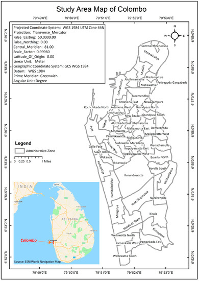
Figure 1.
Sri Lanka context, with details of the study area (Colombo Municipal Council).
The UHI effect in Colombo has been well documented, with strong association between UHI and land cover (particularly green cover) [31,36,38,39], urban growth and density [30,33], urban morphology [40], and urban surface properties [41]. Previous explorations in UHI mitigation include urban form and shade manipulations [35] and increase in urban green space [36,42]. There has been some attempt to quantify the heat hazard in Colombo in the past (using proxy measures for heat hazard, such as land cover [43], LST [30], and HI [44]. However, a recent survey of heat risk assessment in South Asia [45] found no previous attempt in Colombo. Moreover, comprehensive characterisation of the heat risk as defined by the IPCC (hazard, vulnerability, and exposure), has not been attempted in Colombo. Given the high vulnerability of South Asia to heat [46,47], as well as the planning possibilities to mitigate heat risk through climate-sensitive planning, detailed spatial exploration of risk is needed to aid decision-making at local scale.
3. Materials and Methods
In this paper, we aim to highlight the possibility of developing a fine-grained heat risk map in a data-poor region of the world (Colombo, Sri Lanka) to identify local areas of the city where planning resources need to be concentrated to reduce the heat risk. We then explore the likely heat risk reduction through commonly used local climate modifying approaches (densification and green infrastructure) on selected ‘high’ and ‘low’ heat risk areas from this map. The purpose of exploring ‘low risk’ areas is to highlight the contribution of green infrastructure to local cooling, while the purpose of selecting ‘high’ risk areas is to check the likely scale of heat risk reduction possible, by changes to building-generated shading and greening. The former will highlight the causes of low risk (thus, needing protection) while the latter will show the scale of heat risk reduction possible. Together, these could point to a way to develop area-specific planning approaches to mitigate the heat risk.
3.1. Heat Risk Mapping
The process of heat risk mapping followed a five-step workflow:
- Collection of remotely sensed and GIS-based data on the physical and climatological characteristics of the city to estimate the ‘heat hazard’; land use and building quality and type data to derive ‘heat exposure’; and socioeconomic status of the population to characterise ‘heat vulnerability’ (or sensitivity to heat);
- Image processing of all data;
- Spatial correlation check;
- Assignment of weightage and ranking to derive heat risk;
- Multilayer overlay and composite heat risk map (see Figure 2 for a detailed workflow).
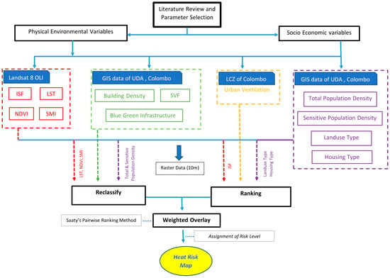 Figure 2. Heat risk mapping workflow.
3.1.1. Data and Assumptions
Table 1 and Table 2 indicate the sources of data, the characterisation of the various parameters used for the determination of heat risk, and the associated assumptions. Where local evidence was available from previous studies on Colombo’s UHI to support the assumptions, these are indicated in parenthesis. Since the aim was to estimate the maximum likely heat risk, we selected climate and environmental data for the driest period (inter-monsoon period 1—see discussions on Colombo context in Section 2.1), when the sun is directly overhead (April) and daytime (see also Section 3.3 for further justifications).

Table 1.
Physical environment and climate data, characterisation, and assumptions.

Table 2.
Socioeconomic data, characterisation, and assumptions.
3.1.2. Image and Data Processing
All the gathered spatial data were processed in a common GIS platform and geographical boundary (administrative wards of the Colombo Municipal Council). All raster were resampled to 10 m from the original 30 m resolution, as explained in Appendix A. The vector data (LCZ, building footprint, green–blue infrastructure and socioeconomic data) within administrative wards were assigned equally to 10 m resolution to bring all data to a common resolution. The satellite image for the Colombo area was obtained on 13 Jan 2017, when the cloud cover was minimal (less than 2.9% of the map area). We used the WGS 84 UTM 44 N projection system for this step. Table 3 and Table 4 show data transformation into usable output layers for the heat risk map. Appendix A provides further details on resampling, LST and NDVI calculations, relevant equations, and normalisation procedures.

Table 3.
Data processing approach—physical environment and climate data.

Table 4.
Data processing approach—socioeconomic data.
3.1.3. Creating LST and NDVI Layers
LST and NDVI are key environmental and climate data. Remotely sensed LST is an average surface temperature per pixel, whereas UHI is usually indicated by air temperature (AT). Fine-grained air temperature data were not available for Colombo, therefore, LST was used as a proxy for heat hazard. As detailed in Appendix A, LST and AT have a linear relationship, which makes LST a reasonable proxy. Conversion of the thermal band’s digital number (DN) values into radiance values is required to create LST from Landsat images. At-satellite brightness temperatures were calculated using these radiance values [51,52]. NDVI on the other hand, is a measure of the health and composition of greenery on a patch of land area. It is calculated from remotely sensed images, using the reflectance in the RED and near-infrared (NIR) bands of the electromagnetic spectrum [53]. Furthermore, the proportion of vegetation was calculated to estimate the land surface emissivity. To adjust LST, the land surface emissivity was determined using the process specified by Sobrino et al. [54]. Finally, the derived LST values were then converted from kelvin to Celsius (°C). We used a single image to derive LST and NDVI, which, in the context of an equatorial climate such as Colombo is appropriate, since annual variation in heat hazard is minimal. Seasonality in terms of temperature and humidity is minimal in Colombo, whereas diurnal variations are larger. Detailed steps and associated equations for the calculations of LST and NDVI as well as the justification for their use, are shown in Appendix A.
3.1.4. Spatial Correlation Check
In the third step, the mapping approach was checked for spatial correlation through Moran’s autocorrelation of each variable and spatial correlation between each variable.
The global Moran’s I statistic assesses spatial autocorrelation based on feature locations and attribute values. In general, global Moran’s I statistics were employed to measure geographic correlation, with positive, negative, and no autocorrelation, as three categories of categorisation statistics [55]. Moran’s I index, expected index, variance, z-score, and p value are the five statistical values produced by spatial autocorrelation. The statistical significance is indicated by the z-score and the p-value. The interpretation of Moran’s I values is shown in Table 5.

Table 5.
Moran’s I value interpretation.
3.1.5. Weight Assignment and Ranking
We used Saaty’s [14] pair-based matrix—AHP—and a nine-level scale for the fourth step in the workflow (weight assignment and ranking). We consulted three local experts familiar with the urban geography of Colombo, using the questionnaire shown in Appendix B, and an average grade of the experts was assigned to each parameter. Experts made comparisons as to the relative importance of the parameters. They indicated on a scale of 1–9 how many times more important or dominant one element was over another with respect to the hazard/vulnerability/exposure criterion or property shown to them. The final priority scales were synthesised by multiplying them by the priority of their parent nodes and adding all such nodes [14]. Table 6 describes the assigned weights for all twelve parameters.

Table 6.
Weights of parameters calculated using AHP method.
Based on expert scores, we applied the interval ranking method to assign weight of sub-class (attribute) for ISF, LCZ, land use type and housing type for the purpose of processing data in the weighted overlay tool of ArcMAP. The ranking is shown below in Table 7, Table 8, Table 9 and Table 10. The ranking order followed a 1–10 scale (1 = low and 10 = high vulnerability to heat).

Table 7.
Ranking of sub-class parameters—ISF.

Table 8.
Ranking of sub-class parameters—LCZ class (see [56] for details of LCZ classes).

Table 9.
Ranking of sub-class parameters—land use type.

Table 10.
Ranking of sub-class parameters—housing type.
3.1.6. Multilayer Overlay and Composite Mapping
After processing all the data, we finally reclassified them on a scale of 1 to 10. The scale indicated an order of heat risk, where 1 was considered the lowest heat risk and 10 was considered the highest risk. Continuous data (LST, NDVI, etc.) were grouped into ten groups of equal intervals, and risk classes (1–10) were assigned on the basis of the assumptions specified in Table 1 and Table 2. Discrete data (such as land use, housing type, etc.) were assigned risk classes according to expert opinion (Table 8, Table 9 and Table 10). We then used the weighted overlay tool in ArcMAP to combine all twelve chosen variables. This produced a heat risk map divided into the said ten classes of heat risk. Since the distribution of heat risk was normal (see Figure 3) we characterised the median range (5–6) as ‘moderate’ heat risk, while the two extremities (1–4 and 8–10) were classified as ‘low’ and ‘high’ heat risk, respectively. The ArcMAP mapping process using model builder is shown in Figure 4.
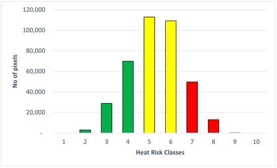
Figure 3.
Distribution of heat risk classes.
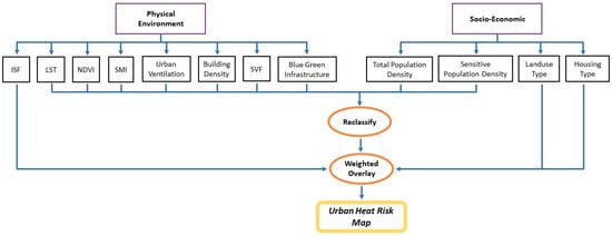
Figure 4.
Model builder of heat risk map in ArcMAP 10.6.
3.2. Estimation of Heat Risk Reduction in Selected ‘High’ and ‘Low’ Risk Areas
The second part of the study focused on estimating the cooling potential of known UHI mitigation approaches (shading and green cover) in parts of the city identified as having different heat risks. Once the heat risk map for Colombo was developed, we selected four blocks of 200 m × 200 m, two each representing ‘High’ and ‘Low’ heat risk as shown in Figure 5. Details of the selected locations are given in Table 11. The justification for their selection is provided in Appendix C, where area statistics of the heat risk in each of the 56 wards of the city of Colombo are shown (we selected areas with the lowest and highest total heat risk).
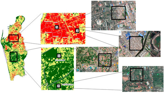
Figure 5.
Selected locations for estimation of heat risk reduction. Note: Please refer to Figure 8 for heat risk categories (green = ‘low,’ yellow = ‘moderate’ and red = ‘high’). The image on left is identical to the heat risk map of Colombo in Figure 8. The purpose is to contextualise the selected locations.

Table 11.
Selected locations for heat risk estimation legend and descriptions.
3.3. Simulation Models and Data
Simulations were carried out using ENVI-met ver. 4.4.6 [15] using the parameters shown in Table 12. Having mapped the heat risk, the purpose of this step was to highlight the differential heat risk reduction possibilities of urban planning options within the same city, highlighting the importance of developing area-specific planning approaches to mitigate the heat risk in Colombo. In other words, would the known heat risk mitigation action (such as manipulating building density, or green cover) work more, or less, in different parts of the city? Are the effects of urban planning options the same in ‘high’ and ‘low’ risk areas?

Table 12.
ENVI-met input parameters for the simulations.
ENVI-met is a three-dimensional non-hydrostatic microclimate model with a typical spatial resolution of 0.5 m up to 10 m, which has already been successfully used in urban heat risk studies in the tropics and has previously been validated in Colombo [32,33]. Figure 6 shows the plan views (and Figure 7, the three-dimensional views) of the selected sites, while the simulation parameters are given in Table 12. Climate data for the initiation of the model were purchased from the Sri Lankan Dept. of Meteorology. Data for the period of 1991 to 2020 indicated April as the hottest month in the current reference period, with April 2016 recording the highest temperature in the past 30 years. We, therefore, selected 15 April 2016 as the simulation date. Simulations started at 6pm on the previous day to allow the model to stabilise. All data were extracted at 1.5 m height to be relevant for the calculation of comfort indices.
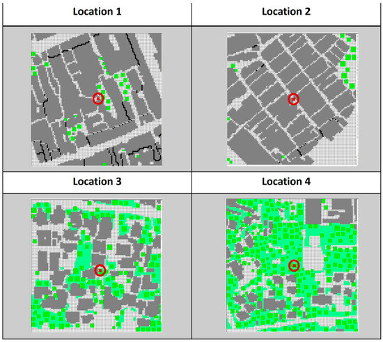
Figure 6.
Simulation models for the base cases with red circles representing locations of data collection.
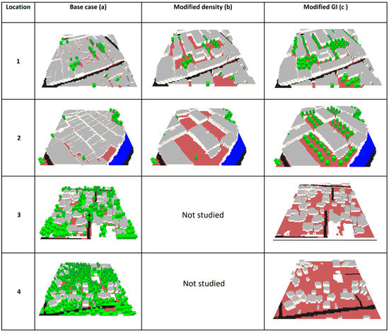
Figure 7.
Three-dimensional view of simulation models. Note: ‘Modified GI’ cases for locations 3 and 4 consisted of the removal of all GI without changes to building volume (see descriptions of cases in Section 3.3).
Simulations in locations 1 and 2 (Table 11, ‘high’ heat risk) consisted of:
- Modified density case—Structures in these locations were often unauthorised and of poor quality, therefore, we converted the area into four-story rectangular blocks by re-arranging the building footprint but maintaining the total building volume (as measured by the floor area ratio—FAR). The Sri Lankan Urban Planning and Building Regulations strictly control FAR [57]; thus, the only way to maintain the FAR when increasing the building height was to reduce its footprint. All buildings except religious buildings and warehouses were, thus, modified (Figure 6 and Figure 7b);
Simulations in locations 3 and 4 (Table 11, ‘low’ heat risk) consisted of:
Simulated data analysed in the next section were obtained from the red circles in Figure 6, representing the middle of the simulation domain.
3.4. Analysis Protocols
Heat stress, especially in tropical outdoor conditions, is notoriously difficult to quantify. No thermal comfort index is fully able to explain heat stress under hot, humid conditions [58]. Among those widely used in hot, humid climates, PET appears to be the most common, especially its modified version which also includes thresholds for tropical heat stress [59]. We used two indicators: MRT and PET. MRT assumes greater importance among these parameters, especially in conditions of high solar angles [60]. MRT, defined as the uniform temperature of an imaginary enclosure in which the radiant heat transfer from the human body equals the radiant heat transfer in the actual non-uniform enclosure [61] is also critical in calculating thermal indices such as PET [62] and UTCI [63]. Given that detailed spatial distribution of heat stress information from ENVI-met is available in MRT, we used MRT as the analysis parameter for spatial analysis of heat stress. MRT is a good proxy for outdoor comfort and is extensively used in the literature [64].
PET is defined as the air temperature in which the heat budget of the human body is balanced in a typical indoor setting (without wind and solar radiation) with the same core and skin temperature as under the complex outdoor conditions to be assessed [60]. ENVI-met provides PET data at selected points and RayMan software was used to calculate the variations in PET over 24 h. Using the MRT information from ENVI-met, we calculated PET for spot analysis of heat stress in the middle of each of the studied domains.
4. Results
Table 13 indicates the spatial correlation between variables. Some high correlations were expected. For example, the well-known coupling between soil moisture and surface temperature [65] was especially true during the daytime, where the water content of upper soil layers and near surface temperature was particularly strong during clear days with reduced wind speeds.

Table 13.
Spatial correlation of selected variables.
Some of the other stronger correlations were logical. Total population density vs. sensitive population density could be expected to be high, assuming these two have similar distributions. Other correlations had support from the literature. For example, the negative relationship between population density and blue–green infrastructure has been well documented [66,67]. While these two variables are generally negatively correlated, the strength of the relationship depends on the population size, type of green infrastructure and location of the city [67]. In the case of Colombo, the available green cover (17% of the total area of the city core [68]) was unequally distributed. The city development plan [68] envisages an increased green cover of 35% by 2030, without changes to either total population or population density. Whether such uniform greening targets are feasible, given the steep increase in green cover needed to meet the target in a short time, remains to be seen.
There are some unique clusters (such as ‘land use type’ vs. ‘housing type’) indicating the socioeconomic characteristics of Colombo. While it is well-known that greener areas are strongly correlated to ‘better quality’ housing types [69], the strong correlation between ‘land use types’ and ‘housing types’ with SVF indicated the low density, open, single-family housing dominated the built form of the city.
Nevertheless, spatial correlation between variables showed that most of them were not strongly correlated (49 out of the 66 correlations were <±0.25). This indicated the usefulness of including all of the chosen variables in estimating heat risk.
4.1. Heat Risk Map of Colombo
Figure 8 shows the final heat risk map we developed for Colombo. The more heavily built-up areas in the centre-north of the city showed high heat risk, while areas with high green and blue infrastructure showed low risk. The fact that the former area also consisted of extremes of socioeconomic conditions (poor quality housing, high population density and high fraction of sensitive population [36]) further added to heat stress inequity in the ‘red’ areas, whereas better housing and lower population density negatively influenced heat stress in the ‘green’ areas in Figure 8.
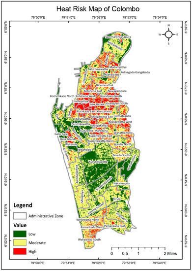
Figure 8.
Heat risk map for Colombo, Sri Lanka.
This was further confirmed by a land cover survey conducted a few years before the Landsat image used for the present heat risk map (2014 vs. 2017) [68]. This study found that Kurunduwatte (the precinct in the middle of Figure 8 and the area of simulation location 3) had the highest concentration of playgrounds, parks and high-function green spaces. A 2017 survey of access to green spaces in Colombo [68] found that over 80% of the Kurunduwatte precinct was covered within 300 m of buffers around green spaces in the area (Figure 6.9 of [69]). Thus, the area was not only well endowed in terms of green spaces, but these were public and highly accessible.
The identified high heat risk areas corresponded well with the action plan of the present Colombo Commercial City Development Plan 2019 to 2030 [70]. The plan recognises some of the areas highlighted by ‘hHigh’ heat risk in Figure 8 (such as Aluthkade East, Aluthkade West, Masangasweediya and Jinthupitya—the first three of which were covered by simulation locations 1 and 2) for their ‘underutilised’ status due to most of the area being occupied by underserved settlements that have encroached on state land and privately owned estates. These areas have emerged informally and in haphazard ways corresponding to socioeconomic processes. A recent stakeholder consultation [71] further highlighted the congested nature of the built form and the lack of open spaces and parks. Our housing type data [36] further indicated the use of temporary building materials, leading to weak capacity for heat adaptation. Unclear land tenure [70] discourages investment in housing improvement. Moreover, it was highlighted that most of these settlements abutted canal fronts that have relatively poor access, and are prone to flooding, thus, resulting in low land values (Figure 79 in Volume 1 and Map 4.9 in Volume 2 [70]). Similarly, the more affluent areas of the city with high land values and low building density corresponded to low heat risk.
The socioeconomic and physical land use linkages between our heat risk map for Colombo showed similarities to studies undertaken in other contexts [72]. Exploring relations between thermal zones and the socioeconomic conditions of the population of Santiago, Chile [73], found that “urban climates are a representation of societal and natural integrated processes. The warmest areas are found in neighbourhoods with high-density social buildings lacking green areas that are located in those areas of the city where lower income population predominates. The coolest areas are located in those neighbourhoods where the most affluent people live; these zones are characterised by the presence of green spaces and lower dwelling densities”.
Additionally, Figure 8 bore a close similarity to a recently published physiological ‘hotspot map’ for Colombo, based solely on thermal stress (‘heat index’) distribution (Figure 6 of [44]). There were striking similarities between the cool spots, but our map is much more spatially fine-grained. Furthermore, the inclusion of vulnerability and exposure parameters added fine details to our heat risk map.
4.2. Applicability of Heat Reduction Approaches in High and Low Heat Risk Areas
Figure 9 shows the daily PET variations at 1.5 m above ground on the hottest day (15 April 2017). While there was no reduction in peak heat stress between the cases, there were clear reductions in the number of hours of heat stress (‘hot’ and ‘very hot’) in the modified cases (i.e., modified density and green cover), especially in ‘high’ heat risk locations. Location 2 (high risk, residential area) had the worst base case with only four hours of neutral conditions and nine hours of very hot conditions, whereas location 4 (low risk, medium density, planned area) had the best base case with eleven hours of neutral conditions and only five hours of very hot conditions. These findings provide further clues to the reasons for the differences: tightly packed built form with barely any vegetation (location 2) and/or lack of open spaces (location 1—high risk, mixed use area), even though both sites have similar built density. Location 4 had higher levels of thermal comfort (or fewer hours of extreme heat stress) than location 3 (low risk, high green, low density) due to high green cover and low paved area (see Table 11). Modification of density in the high heat risk site had no impact on the number of hours of neutral comfort conditions. However, the density variation resulted in a reduction in the number of hours of very hot conditions in location 2. Combining density modification with green cover significantly increased the number of hours with neutral temperature whilst also bringing down the number of hours with high temperatures. Given the low density of building in location 3, the removal of trees made very little difference (Figure 9c).
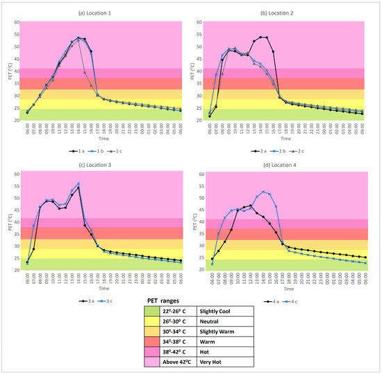
Figure 9.
PET variation for the different scenarios on the simulated day.
Removing all green cover in Location 4 resulted in significantly fewer hours with neutral conditions. This further highlights the importance of vegetation to heat risk reduction at all locations. The results also confirm the ‘accuracy’ of ‘high’ and ‘low’ heat risk areas as classified by our approach, in that the known heat mitigation approaches are able to offer greater cooling in low risk areas than high risk areas.
Figure 10, Figure 11, Figure 12 and Figure 13 show the spatial distribution of MRT at peak daytime (1 p.m. local time) and peak night-time (6 a.m. local time) for all four locations. Unlike the PET values (Figure 9), the MRT distribution had greater variation and could be critical in developing street level heat adaptation strategies.
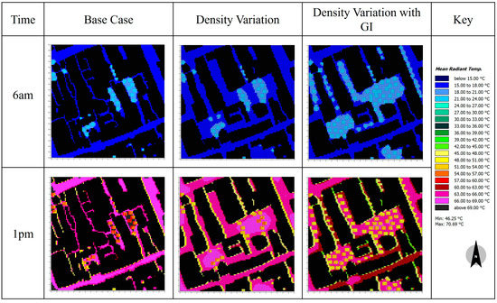
Figure 10.
Spatial MRT variations at location 1 for 6 a.m. and 1 p.m.
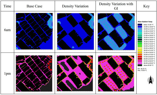
Figure 11.
Spatial MRT variations at location 2 for 6 a.m. and 1 p.m.
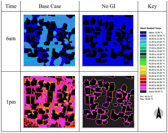
Figure 12.
Spatial MRT variations at location 3 for 6 a.m. and 1 p.m.
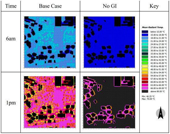
Figure 13.
Spatial MRT variations at location 4 for 6 a.m. and 1 p.m.
Locations 1 and 2 show MRT variations of 15–18 °C across the domain at 6 a.m. except for the slight increase in MRT of 18–21 °C when GI was present. The density modification demonstrated similar results, whereas the introduction of GI resulted in a greater fraction of interstitial spaces showing MRT of 18–21 °C. The inverse was true for locations 3 and 4 at 6 a.m., confirming that the introduction of GI resulted in slightly elevated MRTs between buildings at night-time.
The spatial variations in MRT in the base cases of locations 1 and 2 at 1 p.m. was very high (66–69 °C) along wider streets, and slightly lower (63–66 °C) along narrower streets. The presence of vegetation reduced MRT to 57–60 °C. The shading modification resulted in a slight improvement of MRT in location 1 between buildings, whereas location 2 showed very little difference, highlighting the importance of factors other than shading in optimising thermal comfort. Both locations showed reduced MRT levels of 48–51 °C along the northeast façades, indicating the potential for developing pedestrian activities along these areas. The shading modification combined with green cover in location 1 demonstrated the ideal scenario, with a greater portion of the area at the lower end of the MRT range. This observation was confirmed by the MRT variations in locations 3 and 4, the sparse built form resulting in a relatively lower reduction in MRT, despite the presence of large amounts of GI. As seen in the PET graph (Figure 9) the removal of vegetation in locations 3 and 4 resulted in steep rises in MRT values, highlighting the importance of maintaining green cover to keep these areas cool.
There are several practical implications of these findings:
- The fact that peak heat hazard (thermal stress) was similar in all locations indicates the importance of exposure and sensitivity (i.e., socioeconomic factors) in modulating the heat risk. Given the high correlation between land use classes and ‘housing type’ (with a positive correlation in ‘low’ heat risk areas), improving the housing type and economic conditions of the urban population is an important tool to manage heat risk, rather than merely focusing on reducing temperature;
- The introduction of green cover and shading could reduce heat stress in high heat risk areas, but only if building footprints are arranged to create sufficient interstitial spaces, while maintaining the total built footprint. This implies a more nuanced approach to building footprint regulations in high heat risk areas;
- Local variations in MRT in ‘low’ risk areas showed the importance of green cover. Planning strategies in these areas should, therefore, focus on maintaining the already high green cover.
5. Conclusions
The present work demonstrates the possibility of accurately identifying ‘high’ and ‘low’ heat risk areas in data-poor tropical cities such as Colombo, Sri Lanka, and the varying possibilities of modulating heat stress through planning approaches. Currently available data (remotely sensed temperature, vegetation, and locally-sourced census data) is adequate to develop a detailed spatial understanding of heat risk. While it may not be possible to reduce the peak thermal discomfort, it is possible to reduce the number of hours of heat stress through density and vegetation combinations. The fact that such heat stress reductions are possible without reducing the building footprint points to the possibility of maintaining high building density in a climate-sensitive manner. These could have important planning implications for other hot, humid cities with similar developmental pressures to Colombo.
There are some limitations to the present approach. Only one date (albeit the hottest, least windy, and highest solar radiation day) was selected for heat hazard; although seasonality is limited in Colombo, there may be differences during the rainy season, and this could be explored to better understand the spatial risk profile. However, we have attempted to reduce the effect of seasonality and temporal variation by normalisation, as explained in Appendix A. Another limitation is the lack of fine-grained data on air temperature. In the absence of air temperature, we have used LST as a proxy for heat hazard, which may be a reasonable proxy to air temperature, as shown in Appendix A. Only two urban microclimate modification strategies—shading modification and vegetation—were explored in this study. Other approaches, such as the materiality of the built environment and its contribution to heat vulnerability and/or exposure, were not studied. Additional levels of density, and green cover variations too, need to be studied, to develop a more nuanced understanding of the likely mitigation potential of local planning actions.
In terms of future directions, the interplay between heat hazard and the moderating influence of socioeconomic factors (ranging from public health to energy consumption to economic development and social cohesion) needs more interdisciplinary research to develop a holistic response to the increasing problem of urban- and global-warming-induced heat risk and its mitigation. Work is also needed to develop heat action plans (HAPs) based on heat risk mapping exercises, such as the present study. Additionally, early warning systems, capacity building and community education to raise awareness and take evasive actions to mitigate heat risk are also needed.
Author Contributions
Conceptualisation, R.E.; methodology, R.E., N.P., R.R. and M.J.; software, M.J. and S.O.; validation, S.O., M.Z. and M.J.; formal analysis, N.M., R.E., M.J., R.R. and N.P.; investigation, S.O, M.J., N.M. and M.Z.; resources, R.E.; data curation, M.Z., M.J. and S.O.; writing—original draft preparation, R.E.; writing—review and editing, R.E., N.P., R.R., N.M., M.J. and S.O.; visualisation, M.J., M.Z. and N.M.; supervision, R.E.; project administration, R.E.; funding acquisition, R.E. All authors have read and agreed to the published version of the manuscript.
Funding
This research was partially funded by the Education, Audio-visual and Culture Executive Agency (EACEA) of the EU, grant number 2017-1926.
Institutional Review Board Statement
Not applicable.
Informed Consent Statement
Not applicable.
Data Availability Statement
Restrictions apply to the availability of these data. Data was obtained from Dept. of Census and Statistics, Sri Lanka and are available from the authors with the permission of Dept. of Census and Statistics, Sri Lanka.
Conflicts of Interest
The authors declare no conflict of interest.
Abbreviations
| AHP | Analytical hierarchy process |
| DN | Digital number |
| GIS | Geographic information system |
| HI | Heat index |
| IPCC | Intergovernmental Panel on Climate Change |
| ISF | Impervious surface fraction |
| LCZ | Local climate zone |
| LST | Land surface temperature |
| MRT | Mean radiant temperature |
| NDVI | Normalised difference vegetation index |
| NIR | Near infrared |
| OLI | Operational Land Imager |
| PET | Physiologically equivalent temperature |
| SFDRR | Sendai Framework for Disaster Risk Reduction |
| SMI | Soil moisture index |
| SVF | Sky view factor |
| TIRS | Thermal infrared sensor |
| UC-AnMap | Urban climate analysis map and its corollary |
| UC-ReMap | Urban climate recommendation map |
| UHI | Urban heat island |
| UTCI | Universal thermal climate index |
| UTM | Universal Transverse Mercator |
| WGS | World Geodetic System |
| WUDAPT | World Urban Database Accept Portal Tools |
Appendix A. Explanations of Calculation Processes for LST and NDVI
LST and NDVI retrieval were critical steps of the methodology of the present paper. Radiative transfer equation (as shown in Equation (A6) below) was used. Before using this equation, the digital number needs to be converted to radiance and the sensor’s brightness temperature needs to be known:
Digital number to radiance:
where is the spectral radiance at the sensor’s opening in Watts/(m2·Sr·μm), is the quantised adjusted pixel values in digital number (DN), represents radiance add band, and is the radiance multi band.

Table A1.
Constant used to calculate radiance.
Table A1.
Constant used to calculate radiance.
| Parameter | Landsat 8 Description | Average Values |
|---|---|---|
| Radiance add band 10 | 0.10000 | |
| Radiance add band 11 | ||
| Radiance multi band 10 | 0.0003342 | |
| Radiance multi band 11 |
Brightness temperature:
where represents the satellite temperature in kelvin, is the spectral radiance, while K1 and K2 are the calibrated constant as provided by the Landsat data used by the study.

Table A2.
Constants used to calculate brightness temperature.
Table A2.
Constants used to calculate brightness temperature.
| Calibrated Constant for Landsat 8 | Band | Constant |
|---|---|---|
| K1 | Band 10 | 774.8853 |
| Band 11 | 480.8883 | |
| K2 | Band 10 | 1321.0789 |
| Band 11 | 1201.1442 |
The brightness temperature is affected by atmospheric conditions, which could be improved using NDVI to determine spectral emissivity of various land surface values as per Table A3.

Table A3.
NDVI thresholds for spectral emissivity of land surfaces.
Table A3.
NDVI thresholds for spectral emissivity of land surfaces.
| NDVI Thresholds | Spectral Emissivity of Land Surface (ε) |
|---|---|
| NDVI < −0.185 | 0.995 |
| −0.185 ≤ NDVI ≤ −0.157 | 0.970 |
| −0.157 ≤ NDVI ≤ 0.727 | 1.0094 + Ln(NDVI) |
| NDVI > 0.727 | 0.990 |
Normalised difference vegetation index (NDVI) is given below:
Proportion of vegetation index:
Emissivity:
ε = 0.004PV + 0.986
Land surface temperature:
where is the brightness temperature in kelvin; is the wavelength of emitted radiance (λ = for band 10, and 12 μm for band 11); h is the Planck’s constant (6.626 × 10⁻³⁴ m2kg/s); c represents the velocity of light (2.998 × 10⁸ m/s); is the Boltzmann constant (1.38 × 10⁻²³ J/K), and calculated value is 1.438 × 10⁻² mk.
Conversion of LST from kelvin to degrees Celsius
T°C = LST − 273.15
Table A4 provides details of the satellite image (Operational Land Imager—OLI, and thermal infrared sensors—TIRS) used for the study.

Table A4.
Detail information of the image used for the study.
Table A4.
Detail information of the image used for the study.
| Satellite | Sensor | Metadata | Spatial Resolution | Spectral Band (Wavelength in μm) |
|---|---|---|---|---|
| LANDSAT 8 | OLI and TIRS | Date = 13 January 2017; Scene cloud cover = 2.89% | Bands 1–7, 9 = 30 m Band 8 = 15 m Band 10 and 11 = 100 m (re-sampled to 30 m) | Band 1—Coastal aerosol (0.43–0.45) |
| Band 2—Blue (0.45–0.51) | ||||
| Band 3—Green (0.53–0.59) | ||||
| Band 4—Red (0.64–0.67) | ||||
| Band 5—Near infrared (NIR) (0.85–0.88) | ||||
| Band 6—SWIR1 (1.57–1.65) | ||||
| Band 7—SWIR2 (2.11–2.29) | ||||
| Band 8—Panchromatic (0.50–0.68) | ||||
| Band 9—Cirrus (1.36–1.38) | ||||
| Band 10—TIRS1 (10.60–11.19) | ||||
| Band 11—TIRS2 (11.50–12.51) |
Source: https://www.usgs.gov/media/images/landsat-8-oli-and-tirs-and-their-uses. (accessed on 19 December 2022.)
As indicated in Table A4, the cloud cover contamination was minimal, requiring no further treatment. In terms of resampling, we further resampled the 30 m resolution provided by the data provider into 10 m using the bilinear interpolation method in ArcGIS software. Bilinear interpolation calculates the value of each pixel by averaging the values of the surrounding four pixels (weighted for distance). Such interpolation is appropriate for continuous data, whereas other resampling methods such as ‘nearest neighbour’ or ‘majority resampling’ are more appropriate for discrete data. Although the cubic interpolation method is also applicable for continuous data, its use of 16 surrounding pixels for weighted average tends to reduce the variations in data. Therefore, we used the bilinear method to resample the LST data by considering closest temperature values of LST as well as taking into account the nearest temperature values with higher weight (Source: https://desktop.arcgis.com/en/arcmap/latest/tools/data-management-toolbox/resample.htm, accessed on 19 December 2022.).
Appendix A.1. Soil Moisture Index (SMI)
The dry edge and wet edge LST and NDVI connections provided confidence that soil moisture could be determined using the LST–NDVI space [74]. The formula (Equation (A9)) to estimate soil moisture index within the space of LST–NDVI was previously proposed [74].
where is the maximum LST value, is the minimum LST value, SMI is the soil moisture index, while a1, a2, and b1, b2 are empirical parameters for both the dry and wet margins that can be determined by linear regression of known remotely sensed data.
Appendix A.2. Impervious Surface Extraction
Impervious surface areas of the study area were extracted using the supervised classification technique of Landsat 8 OLI Satellite imagery. Based on spectral reflectance of surface properties in different colour bands, the surface features were classified into impervious (built-up) and pervious (water, vegetation, and bare land) zones. Maximum likelihood classification technique was used for interpolation of spectral signature.
Appendix A.3. LST Validation
Validity and accuracy of satellite-derived output on surface temperature are necessary conditions to increase the reliability of extracted LST. Given the absence of in situ measurements of local surface and air temperatures in our present study, the process of validation of temperature data necessarily relied on secondary sources in similar climates.
A recent study [75] showed that satellite-derived longwave upward radiation of Landsat has a bias of 1.9 kelvin and RMSE of 1.2 kelvin. Although the temperature results from the NOAA-AVHRR platform and MODIS sensor are known for better accuracy, their spatial resolution is poor. The higher spatial resolution of Landsat products is more appropriate for a detailed heat risk mapping study such as the present paper. A further study [76] found a high degree of agreement between the satellite-retrieved surface temperature and the ground-based LST observations. The correlation, root mean square (RMS) difference, and standard deviation for the two sets of data were estimated as 0.89, 0.5 °C, and approximately 0.72 °C, respectively. Another study [77] also found similar patterns between satellite-derived LST and ground-measured surface temperature across 13 stations. Additional studies [78] have considered satellite-derived data as being well representative of UHI on heterogeneous surfaces. There is also evidence that there is a linear relationship between atmospheric and surface urban heat island [79]. Although the intensity of air temperature heat island is lower—compared with surface temperature heat island—there was a linear trend across the study area. As such, the use of satellite-derived LST can be considered as a justified proxy indicator for surface urban heat intensity, which, at worst, may have a linear relationship with atmospheric urban heat island.
Appendix A.4. Normalisation of LST
Given that we used one satellite image to derive the heat hazard, the present study used normalisation technique to reduce the effect of seasonality and temporal variation by smoothing the pixel values. A similar approach [79] used different statistical methods to represent spatial non-stationarity of surface temperature across the city. However, the present study used the normalised ratio scale (NRS) method according to Equation (A11) to represent the LST value as a source information for surface thermal characteristics by normalising the effect of seasonal and temporal variations.
Compared with other investigated methods, NRS produces less discrepancy across the year [80]. Therefore, this method was adopted in this study to ensure non-stationarity; in addition, the LST pixel values had a lesser, and acceptable, range of annual anomaly.
Appendix B. Analytical Hierarchical Process (AHP) Matrix Used in the Study
| Relative Comparison | |||||||||
| Land Surface Temperature | NDVI | Building Density | Sky View Factor | Uninterrupted Wind Flow | Impervious Surface Fraction | Soil Moisture Index | Blue Infrastructure | Instruction | |
| Land Surface Temperature | 1 | 3 | This matrix aims to | ||||||
| NDVI | 0.333333333 | 1 | derive the relative importance of environ- | ||||||
| Building Density | #DIV/0! | 1 | mental and socio- | ||||||
| Sky View Factor | #DIV/0! | 1 | 0.2 | economic variables to the urban heat island | |||||
| Uninterrupted Wind Flow | #DIV/0! | 1 | phenomenon. In | ||||||
| Impervious Surface Fraction | #DIV/0! | 1 | this worksheet, you are asked to rate | ||||||
| Soil Moisture Index | #DIV/0! | 1 | the relative importance of each of | ||||||
| Blue Infrastructure | #DIV/0! | 1 | the eight variables | ||||||
| Total of Column | #DIV/0! | against each other, on a scale of 1 to 9 | |||||||
Instructions
This matrix aims to derive the relative importance of environmental and socioeconomic variables to the urban heat island phenomenon. In this worksheet, you are asked to rate the relative importance of each of the eight variables against each other, on a scale of 1 to 9.
Example 1.Cell no D4.
Regarding UHI, if it is considered that land surface temperature is three times (out of nine) more important than NDVI, then put 3 in this cell (LST to NDVI).
| Weight Assignment | ||||||||||
| Land Surface Temperature | NDVI | Building Density | Sky View Factor | Uninterrupted Wind Flow | Impervious Surface Fraction | Soil Moisture Index | Blue Infrastructure | Average of Row | Weight (% of av of row) | |
| Land Surface Temperature | ||||||||||
| NDVI | ||||||||||
| Building Density | ||||||||||
| Sky View Factor | ||||||||||
| Uninterrupted Wind Flow | ||||||||||
| Impervious Surface Fraction | ||||||||||
| Soil Moisture Index | ||||||||||
| Blue Infrastructure | ||||||||||
| Total | ||||||||||
| Relative Comparison | |||||
| Population Density | Land Use of Building | Sensitive Population Density | Household Income Level | Vehicular Pollution Dispersion (Mobility) | |
| Population Density | 1 | ||||
| Land Use of Building | 1 | ||||
| Sensitive Population Density | 1 | ||||
| Household Income Level | 1 | ||||
| Vehicular Pollution Dispersion (Mobility) | 1 | ||||
| Total of Column | |||||
| Weight Assignment | |||||||
| Population Density | Land Use of Building | Sensitive Population Density | Household Income Level | Vehicular Pollution Dispersion (Mobility) | Average of Row | Weight (% of av of row) | |
| Population Density | |||||||
| Land Use of Building | |||||||
| Sensitive Population Density | |||||||
| Household Income Level | |||||||
| Vehicular Pollution Dispersion (Mobility) | |||||||
| Total | |||||||
| Relative Comparison | ||
| Environmental | Socioeconomic | |
| Environmental | 1 | |
| Socioeconomic | 1 | |
| Total of Column | ||
| Weight Assignment | ||||
| Environmental | Socioeconomic | Average of Row | Weight (% of av of row) | |
| Environmental | ||||
| Socioeconomic | ||||
| Total | ||||
Appendix C. Summary Heat Risk Statistics by Administrative Zones of Colombo

Table A5.
Colombo municipal council area—zonal statistics of heat risk.
Table A5.
Colombo municipal council area—zonal statistics of heat risk.
| Administrative Zone | Zone Code | Count (Pixels) | Area (m2) | Heat Risk | ||||||||
|---|---|---|---|---|---|---|---|---|---|---|---|---|
| Min | Max | Range | Mean | Std | Variety | Majority | Minority | Median | ||||
| Aluthkade West | 2 | 1464 | 146,400.00 | 5 | 9 | 4 | 7.352 | 0.792 | 5 | 8 | 9 | 8 |
| Kochchikade South | 14 | 2270 | 227,000.00 | 5 | 9 | 4 | 7.235 | 0.814 | 5 | 8 | 9 | 7 |
| Kochchikade North | 13 | 2264 | 226,400.00 | 5 | 8 | 3 | 7.174 | 0.743 | 4 | 7 | 5 | 7 |
| Masangasweediya | 24 | 2584 | 258,400.00 | 5 | 8 | 3 | 7.146 | 0.715 | 4 | 7 | 5 | 7 |
| Jinthupitiya | 10 | 1991 | 199,100.00 | 5 | 8 | 3 | 7.119 | 0.654 | 4 | 7 | 5 | 7 |
| Nawagampura | 27 | 1258 | 125,800.00 | 5 | 9 | 4 | 7.068 | 0.824 | 5 | 7 | 9 | 7 |
| Aluthkade East | 1 | 2777 | 277,700.00 | 5 | 8 | 3 | 7.027 | 0.854 | 4 | 7 | 5 | 7 |
| New Bazaar | 28 | 5029 | 502,900.00 | 5 | 9 | 4 | 6.913 | 0.814 | 5 | 7 | 9 | 7 |
| Grandpass North | 6 | 3344 | 334,400.00 | 5 | 8 | 3 | 6.788 | 0.832 | 4 | 7 | 5 | 7 |
| Grandpass South | 7 | 5279 | 527,900.00 | 4 | 9 | 5 | 6.756 | 0.999 | 6 | 7 | 4 | 7 |
| Slave Island | 32 | 1123 | 112,300.00 | 4 | 8 | 4 | 6.695 | 0.860 | 5 | 7 | 4 | 7 |
| Khettarama | 12 | 3332 | 333,200.00 | 4 | 8 | 4 | 6.601 | 1.026 | 5 | 6 | 4 | 7 |
| Kotahena West | 16 | 3077 | 307,700.00 | 4 | 8 | 4 | 6.561 | 0.816 | 5 | 7 | 4 | 7 |
| Panchikawatta | 29 | 2316 | 231,600.00 | 4 | 8 | 4 | 6.561 | 0.868 | 5 | 7 | 4 | 7 |
| Maligakanda | 20 | 2379 | 237,900.00 | 5 | 8 | 3 | 6.478 | 0.808 | 4 | 6 | 5 | 6 |
| Madampitiya | 18 | 2802 | 280,200.00 | 4 | 9 | 5 | 6.408 | 0.965 | 6 | 6 | 9 | 6 |
| Maradana | 23 | 1946 | 194,600.00 | 4 | 8 | 4 | 6.357 | 0.938 | 5 | 7 | 4 | 6 |
| Dematagoda | 38 | 7311 | 731,100.00 | 4 | 8 | 4 | 6.277 | 0.916 | 5 | 7 | 4 | 6 |
| Kotahena East | 15 | 3411 | 341,100.00 | 4 | 8 | 4 | 6.269 | 0.732 | 5 | 7 | 8 | 6 |
| Kuppiyawatta West | 45 | 3671 | 367,100.00 | 4 | 8 | 4 | 6.252 | 0.796 | 5 | 6 | 4 | 6 |
| Maligawatta West | 22 | 2666 | 266,600.00 | 5 | 8 | 3 | 6.201 | 0.807 | 4 | 6 | 8 | 6 |
| Pamankada West | 50 | 6103 | 610,300.00 | 4 | 7 | 3 | 6.188 | 0.688 | 4 | 6 | 4 | 6 |
| Sammanthranapura | 31 | 1721 | 172,100.00 | 3 | 8 | 5 | 6.181 | 0.957 | 6 | 6 | 3 | 6 |
| Modara | 26 | 7795 | 779,500.00 | 3 | 8 | 5 | 6.047 | 0.948 | 6 | 6 | 3 | 6 |
| Keselwatta | 11 | 3062 | 306,200.00 | 4 | 8 | 4 | 5.960 | 0.893 | 5 | 6 | 4 | 6 |
| Wanathamulla | 52 | 6071 | 607,100.00 | 4 | 8 | 4 | 5.922 | 0.891 | 5 | 6 | 8 | 6 |
| Wellawatta South | 54 | 6377 | 637,700.00 | 4 | 7 | 3 | 5.761 | 0.804 | 4 | 6 | 4 | 6 |
| Aluthmawatha | 3 | 6390 | 639,000.00 | 3 | 8 | 5 | 5.751 | 0.921 | 6 | 6 | 3 | 6 |
| Kuppiyawatta East | 44 | 5730 | 573,000.00 | 4 | 8 | 4 | 5.711 | 0.923 | 5 | 6 | 8 | 6 |
| Maligawatta East | 21 | 6325 | 632,500.00 | 4 | 8 | 4 | 5.591 | 0.991 | 5 | 5 | 8 | 5 |
| Borella South | 37 | 6562 | 656,200.00 | 4 | 7 | 3 | 5.580 | 0.766 | 4 | 6 | 4 | 6 |
| Bloemendhal | 4 | 10,062 | 1,006,200.00 | 3 | 8 | 5 | 5.579 | 0.941 | 6 | 5 | 3 | 6 |
| Mahawatta | 19 | 4903 | 490,300.00 | 3 | 8 | 5 | 5.569 | 0.964 | 6 | 5 | 3 | 5 |
| Wellawatta North | 53 | 9443 | 944,300.00 | 3 | 7 | 4 | 5.564 | 0.885 | 5 | 6 | 3 | 6 |
| Borella North | 36 | 9010 | 901,000.00 | 4 | 8 | 4 | 5.506 | 0.879 | 5 | 5 | 8 | 5 |
| Pettah | 30 | 6854 | 685,400.00 | 3 | 8 | 5 | 5.465 | 0.964 | 6 | 5 | 3 | 5 |
| Kollupitiya | 43 | 6821 | 682,100.00 | 3 | 7 | 4 | 5.415 | 0.842 | 5 | 6 | 3 | 5 |
| Milagiriya | 47 | 10,639 | 1,063,900.00 | 3 | 7 | 4 | 5.393 | 0.747 | 5 | 6 | 3 | 5 |
| Pamankada East | 49 | 8340 | 834,000.00 | 4 | 7 | 3 | 5.358 | 0.833 | 4 | 5 | 7 | 5 |
| Lunupokuna | 17 | 10,652 | 1,065,200.00 | 3 | 8 | 5 | 5.241 | 0.861 | 6 | 5 | 8 | 5 |
| Bambalapitiya | 35 | 12,479 | 1,247,900.00 | 3 | 7 | 4 | 5.190 | 0.790 | 5 | 6 | 7 | 5 |
| Wekanda | 34 | 3532 | 353,200.00 | 3 | 8 | 5 | 5.187 | 1.354 | 6 | 4 | 8 | 5 |
| Havelock Town | 40 | 12,911 | 1,291,100.00 | 3 | 7 | 4 | 5.124 | 0.802 | 5 | 5 | 7 | 5 |
| Kirulapone | 42 | 12,621 | 1,262,100.00 | 3 | 7 | 4 | 5.097 | 0.800 | 5 | 5 | 3 | 5 |
| Kirula | 41 | 16,199 | 1,619,900.00 | 3 | 7 | 4 | 5.094 | 0.827 | 5 | 5 | 3 | 5 |
| Ibbanwala | 9 | 7504 | 750,400.00 | 3 | 7 | 4 | 5.084 | 0.889 | 5 | 5 | 7 | 5 |
| Peliyagoda Gangabada | 55 | 205 | 20,500.00 | 4 | 7 | 3 | 4.976 | 0.435 | 4 | 5 | 7 | 5 |
| Mattakkuliya | 25 | 19,754 | 1,975,400.00 | 2 | 8 | 6 | 4.835 | 1.028 | 7 | 5 | 8 | 5 |
| Narahenpita | 48 | 7790 | 779,000.00 | 3 | 7 | 4 | 4.797 | 0.994 | 5 | 5 | 7 | 5 |
| Hunupitiya | 8 | 7591 | 759,100.00 | 3 | 7 | 4 | 4.645 | 1.301 | 5 | 3 | 7 | 5 |
| Suduwella | 33 | 7886 | 788,600.00 | 3 | 8 | 5 | 4.569 | 0.967 | 6 | 4 | 8 | 4 |
| Fort | 56 | 12,624 | 1,262,400.00 | 2 | 7 | 5 | 4.426 | 1.066 | 6 | 4 | 2 | 4 |
| Thimbirigasyaya | 51 | 18,590 | 1,859,000.00 | 3 | 7 | 4 | 4.340 | 0.931 | 5 | 4 | 7 | 4 |
| Galle Face | 5 | 4733 | 473,300.00 | 3 | 8 | 5 | 4.209 | 0.909 | 6 | 4 | 8 | 4 |
| Kurunduwatta | 46 | 35,513 | 3,551,300.00 | 2 | 7 | 5 | 4.006 | 1.012 | 6 | 3 | 7 | 4 |
| Gothamipura | 39 | 11,211 | 1,121,100.00 | 2 | 7 | 5 | 3.903 | 1.158 | 6 | 3 | 7 | 4 |
| Bold indicates selected locations | ||||||||||||
| Bold indicates selected locations | ||||||||||||
References
- Jay, O.; Capon, A.; Berry, P.; Broderick, C.; de Dear, R.; Havenith, G.; Honda, Y.; Kovats, R.S.; Ma, W.; Malik, A.; et al. Reducing the health effects of hot weather and heat extremes: From personal cooling strategies to green cities. Lancet 2021, 398, 709–724. [Google Scholar] [CrossRef]
- IPCC. Climate Change 2021: The Physical Science Basis, Contribution of Working Group I to the Sixth Assessment Report of the Intergovernmental Panel on Climate Change; Masson-Delmotte, V.P., Zhai, A., Pirani, S.L., Connors, C., Péan, S., Berger, N., Caud, Y., Chen, L., Goldfarb, M.I., Gomis, M., et al., Eds.; Cambridge University Press: Cambridge, UK, 2021. [Google Scholar]
- Hamdi, R.; Kusaka, H.; Doan, Q.-V.; Cai, P.; He, H.; Luo, G.; Kuang, W.; Caluwaerts, S.; Duchêne, F.; Van Schaeybroek, B.; et al. The State-of-the-Art of Urban Climate Change Modeling and Observations. Earth Syst. Environ. 2020, 4, 631–646. [Google Scholar] [CrossRef]
- Shreevastava, A.; Prasanth, S.; Ramamurthy, P.; Rao, P.S.C. Scale-dependent response of the urban heat island to the European heatwave of 2018. Environ. Res. Lett. 2021, 16, 104021. [Google Scholar] [CrossRef]
- Rogers, C.D.; Gallant, A.J.; Tapper, N.J. Is the urban heat island exacerbated during heatwaves in southern Australian cities? Theor. Appl. Clim. 2019, 137, 441–457. [Google Scholar] [CrossRef]
- IPCC. Climate Change 2022: Impacts, Adaptation, and Vulnerability. Contribution of Working Group II to the Sixth Assessment Report of the Intergovernmental Panel on Climate Change; Pörtner, H.-O., Roberts, D., Tignor, M., Poloczanska, E., Mintenbeck, K., Alegría, A., Craig, M., Langsdorf, S., Löschke, S., Möller, V., et al., Eds.; Cambridge University Press: Cambridge, UK, 2022. [Google Scholar]
- Cardona, O.D.; van Aalst, M.K.; Birkmann, J.; Fordham, M.; McGregor, G.; Perez, R.; Pulwarty, R.S.; Schipper, E.L.F.; Sinh, B.T. Determinants of risk: Exposure and vulnerability. In Managing the Risks of Extreme Events and Disasters to Advance Climate Change Adaptation; Field, C.B., Barros, V., Stocker, T.F., Qin, D., Dokken, D.J., Ebi, K.L., Mastrandrea, M.D., Mach, K.J., Plattner, G.-K., Allen, S.K., et al., Eds.; A Special Report of Working Groups I and II of the Intergovernmental Panel on Climate Change (IPCC); Cambridge University Press: Cambridge, UK; New York, NY, USA, 2012; pp. 65–108. [Google Scholar]
- Rosenthal, J.K.; Kinney, P.L.; Metzger, K.B. Intra-urban vulnerability to heat-related mortality in New York City, 1997–2006. Health Place 2014, 30, 45–60. [Google Scholar] [CrossRef]
- Keramitsoglou, I.; Sismanidis, P.; Analitis, A.; Butler, T.; Founda, D.; Giannakopoulos, C.; Giannatou, E.; Karali, A.; Katsouyanni, K.; Kendrovski, V.; et al. Urban thermal risk reduction: Developing and implementing spatially explicit services for resilient cities. Sustain. Cities Soc. 2017, 34, 56–68. [Google Scholar] [CrossRef]
- Tomlinson, C.J.; Chapman, L.; Thornes, J.E.; Baker, C.J. Including the urban heat island in spatial heat health risk assessment strategies: A case study for Birmingham, UK. Int. J. Health Geogr. 2011, 10, 42. [Google Scholar] [CrossRef]
- Kamal, N.I.A.; Ash’Aari, Z.H.; Abdullah, A.M.; Kusin, F.M.; Yusuff, F.M.; Sharaai, A.H.; Muharam, F.M.; Ariffin, N.A.M. Extreme heat vulnerability assessment in tropical region: A case study in Malaysia. Clim. Dev. 2021, 14, 472–486. [Google Scholar] [CrossRef]
- De Perez, E.C.; van Aalst, M.; Bischiniotis, K.; Mason, S.; Nissan, H.; Pappenberger, F.; Stephens, E.; Zsoter, E.; Hurk, B.V.D. Global predictability of temperature extremes. Environ. Res. Lett. 2018, 13, 054017. [Google Scholar] [CrossRef]
- Oppermann, E.; Strengers, Y.; Maller, C.; Rickards, L.; Brearley, M. Beyond Threshold Approaches to Extreme Heat: Repositioning Adaptation as Everyday Practice. Weather. Clim. Soc. 2018, 10, 885–898. [Google Scholar] [CrossRef]
- Saaty, T.L.; Peniwati, K.; Shang, J.S. The analytic hierarchy process and human resource allocation: Half the story. Math. Comput. Model. 2007, 46, 1041–1053. [Google Scholar] [CrossRef]
- ENVI-met. ENVI-met. A Holistic Microclimate Modelling System. Available online: https://envi-met.info/doku.php?id=root:start (accessed on 19 December 2022).
- Li, Z.; Hu, J.; Meng, R.; He, G.; Xu, X.; Liu, T.; Zeng, W.; Li, X.; Xiao, J.; Huang, C.; et al. The association of compound hot extreme with mortality risk and vulnerability assessment at fine-spatial scale. Environ. Res. 2021, 198, 111213. [Google Scholar] [CrossRef]
- Baumüller, J.; Reuter, U. Demands and Requirements on a Climate Atlas for Urban Planning and Design; Office of Environmental Protection: Stuttgart, Germany, 1999. [Google Scholar]
- VDI. VDI-Guideline 3787, Part 1, Environmental Meteorology-Climate and Air Pollution Maps for Cities and Regions; VDI, Beuth Verlag: Berlin, Germany, 1997. [Google Scholar]
- Demuzere, M.; Kittner, J.; Bechtel, B. LCZ Generator: A Web Application to Create Local Climate Zone Maps. Front. Environ. Sci. 2021, 9, 637455. [Google Scholar] [CrossRef]
- Bechtel, B.; Alexander, P.J.; Böhner, J.; Ching, J.; Conrad, O.; Feddema, J.; Mills, G.; See, L.; Stewart, I. Mapping Local Climate Zones for a Worldwide Database of the Form and Function of Cities. ISPRS Int. J. Geo-Inf. 2015, 4, 199–219. [Google Scholar] [CrossRef]
- Perera, N.G.R.; Emmanuel, R. A “Local Climate Zone” based approach to urban planning in Colombo, Sri Lanka. Urban Clim. 2018, 23, 188–203. [Google Scholar] [CrossRef]
- Quan, S.J.; Bansal, P. A systematic review of GIS-based local climate zone mapping studies. Build. Environ. 2021, 196, 107791. [Google Scholar] [CrossRef]
- Bechtel, B.; Alexander, P.J.; Beck, C.; Böhner, J.; Brousse, O.; Ching, J.; Demuzere, M.; Fonte, C.; Gál, T.; Hidalgo, J.; et al. Generating WUDAPT Level 0 data—Current status of production and evaluation. Urban Clim. 2019, 27, 24–45. [Google Scholar] [CrossRef]
- Kotharkar, R.; Ghosh, A.; Kotharkar, V. Estimating summertime heat stress in a tropical Indian city using Local Climate Zone (LCZ) framework. Urban Clim. 2021, 36, 100784. [Google Scholar] [CrossRef]
- Shi, Y.; Ren, C.; Luo, M.; Ching, J.; Li, X.; Bilal, M.; Fang, X.; Ren, Z. Utilizing world urban database and access portal tools (WUDAPT) and machine learning to facilitate spatial estimation of heatwave patterns. Urban Clim. 2021, 36, 100797. [Google Scholar] [CrossRef]
- Benz, S.A.; Burney, J.A. Widespread Race and Class Disparities in Surface Urban Heat Extremes Across the United States. Earth’s Futur. 2021, 9, e2021EF002016. [Google Scholar] [CrossRef]
- Chakraborty, T.; Hsul, A.; Manyal, D.; Sheriff, G. Disproportionately higher exposure to urban heat in lower-income neighbor-hoods: A multi-city perspective. Environ. Res. Lett. 2019, 14, 105003. [Google Scholar]
- Li, X.-X. Heat wave trends in Southeast Asia during 1979–2018: The impact of humidity. Sci. Total. Environ. 2020, 721, 137664. [Google Scholar] [CrossRef]
- Parkes, B.; Buzan, J.R.; Huber, M. Heat stress in Africa under high intensity climate change. Int. J. Biometeorol. 2022, 66, 1531–1545. [Google Scholar] [CrossRef]
- Fonseka, H.; Zhang, H.; Sun, Y.; Su, H.; Lin, H.; Lin, Y. Urbanization and Its Impacts on Land Surface Temperature in Colombo Metropolitan Area, Sri Lanka, from 1988 to 2016. Sens. 2019, 11, 957. [Google Scholar] [CrossRef]
- Ranagalage, M.; Estoque, R.C.; Murayama, Y. An Urban Heat Island Study of the Colombo Metropolitan Area, Sri Lanka, Based on Landsat Data (1997–2017). ISPRS Int. J. Geo. Inf. 2017, 6, 189. [Google Scholar] [CrossRef]
- Subasinghe, S.; Estoque, R.C.; Murayama, Y. Spatiotemporal Analysis of Urban Growth Using GIS and Remote Sensing: A Case Study of the Colombo Metropolitan Area, Sri Lanka. ISPRS Int. J. Geo. Inf. 2016, 5, 197. [Google Scholar] [CrossRef]
- Emmanuel, R. Thermal comfort implications of urbanization in a warm-humid city: The Colombo Metropolitan Region (CMR), Sri Lanka. Build. Environ. 2005, 40, 1591–1601. [Google Scholar] [CrossRef]
- Johansson, E.; Emmanuel, R. The influence of urban design on outdoor thermal comfort in the hot, humid city of Colombo, Sri Lanka. Int. J. Biometeorol. 2006, 51, 119–133. [Google Scholar] [CrossRef]
- Emmanuel, R.; Rosenlund, H.; Johansson, E. Urban shading-a design option for the tropics? A study in Colombo, Sri Lanka. Int. J. Clim. 2007, 27, 1995–2004. [Google Scholar] [CrossRef]
- Maheng, D.; Ducton, I.; Lauwaet, D.; Zevenbergen, C.; Pathirana, A. The Sensitivity of Urban Heat Island to Urban Green Space—A Model-Based Study of City of Colombo, Sri Lanka. Atmosphere 2019, 10, 151. [Google Scholar] [CrossRef]
- Ranagalage, M.; Estoque, R.C.; Zhang, X.; Murayama, Y. Spatial Changes of Urban Heat Island Formation in the Colombo District, Sri Lanka: Implications for Sustainability Planning. Sustainability 2018, 10, 1367. [Google Scholar] [CrossRef]
- Deptartman of Census and Statistics (DCS), Census of Population and Housing-2012, Final Report. 2012. Available online: https://www.statistics.gov.lk/Population/StaticalInformation/CPH2011/CensusPopulationHousing2012-FinalReport (accessed on 19 December 2022.).
- Emmanuel, R. Assessment of Impact of Land Cover Changes on Urban Bioclimate: The Case of Colombo, Sri Lanka. Arch. Sci. Rev. 2003, 46, 151–158. [Google Scholar] [CrossRef]
- Emmanuel, R.; Johansson, E. The influence of urban morphology and sea breeze on hot, humid microclimate: The case of Colombo, Sri Lanka. Clim. Res. 2006, 30, 189–200. [Google Scholar] [CrossRef]
- Emmanuel, R.; Fernando, H.J.S. Urban heat islands in humid and arid climates: Role of urban form and thermal properties in Colombo, Sri Lanka and Phoenix, USA. Clim. Res. 2007, 34, 241–251. [Google Scholar] [CrossRef]
- Herath, H.; Halwatura, R.; Jayasinghe, G. Evaluation of green infrastructure effects on tropical Sri Lankan urban context as an urban heat island adaptation strategy. Urban For. Urban Green. 2018, 29, 212–222. [Google Scholar] [CrossRef]
- Jayasinghe, P.; Raghavan, V.; Yonezawa, G. Exploration of expansion patterns and prediction of urban growth for Colombo City, Sri Lanka. Spat. Inf. Res. 2021, 29, 465–478. [Google Scholar] [CrossRef]
- Perera, T.A.N.T.; Nayanajith, T.M.D.; Jayasinghe, G.Y.; Premasiri, H.D.S. Identification of thermal hotspots through heat index determination and urban heat island mitigation using ENVImet numerical micro climate model. Model. Earth Syst. Environ. 2021, 8, 209–226. [Google Scholar] [CrossRef]
- Dimitrova, A.; Ingole, V.; Basagaña, X.; Ranzani, O.; Milà, C.; Ballester, J.; Tonne, C. Association between ambient temperature and heat waves with mortality in South Asia: Systematic review and meta-analysis. Environ. Int. 2020, 146, 106170. [Google Scholar] [CrossRef]
- Byers, E.; Gidden, M.; Leclère, D.; Balkovic, J.; Burek, P.; Ebi, K.; Greve, P.; Grey, D.; Havlik, P.; Hillers, A.; et al. Global exposure and vulnerability to multi-sector development and climate change hotspots. Environ. Res. Lett. 2018, 13, 055012. [Google Scholar] [CrossRef]
- Mora, C.; Dousset, B.; Caldwell, I.R.; Powell, F.E.; Geronimo, R.C.; Bielecki, C.R.; Counsell, C.W.W.; Dietrich, B.S.; Johnston, E.T.; Louis, L.V.; et al. Global risk of deadly heat. Nat. Clim. Chang. 2017, 7, 501–506. [Google Scholar] [CrossRef]
- Senanayake, I.; Welivitiya, W.; Nadeeka, P. Remote sensing based analysis of urban heat islands with vegetation cover in Colombo city, Sri Lanka using Landsat-7 ETM+ data. Urban Clim. 2013, 5, 19–35. [Google Scholar] [CrossRef]
- Allender, S.; Wickramasinghe, K.; Goldacre, M.; Matthews, D.; Katulanda, P. Quantifying Urbanization as a Risk Factor for Noncommunicable Disease. J. Urban Health 2011, 88, 906–918. [Google Scholar] [CrossRef]
- Rhew, I.C.; Stoep, A.V.; Kearney, A.; Smith, N.L.; Dunbar, M.D. Validation of the Normalized Difference Vegetation Index as a Measure of Neighborhood Greenness. Ann. Epidemiol. 2011, 21, 946–952. [Google Scholar] [CrossRef]
- Weng, Q.; Lu, D.; Schubring, J. Estimation of land surface temperature–vegetation abundance relationship for urban heat island studies. Remote Sens. Environ. 2004, 89, 467–483. [Google Scholar] [CrossRef]
- Liu, H.; Weng, Q. Enhancing temporal resolution of satellite imagery for public health studies: A case study of West Nile Virus outbreak in Los Angeles in 2007. Sens. Environ. 2012, 117, 57–71. [Google Scholar] [CrossRef]
- Orhan, O.; Ekercin, S.; Dadaser-Celik, F. Use of Landsat Land Surface Temperature and Vegetation Indices for Monitoring Drought in the Salt Lake Basin Area, Turkey. Sci. World J. 2014, 2014, 142939. [Google Scholar] [CrossRef]
- Sobrino, J.A.; Jiménez-Muñoz, J.C.; Paolini, L. Land surface temperature retrieval from LANDSAT TM 5. Sens. Environ. 2004, 90, 434–440. [Google Scholar] [CrossRef]
- Boots, B.N.; Getis, A. Point Pattern Analysis; Newbury Park: Sage, CA, USA, 1988. [Google Scholar]
- Stewart, I.D.; Oke, T.R. Local Climate Zones for Urban Temperature Studies. Bull. Am. Meteorol. Soc. 2012, 93, 1879–1900. [Google Scholar] [CrossRef]
- Goverment of Sri Lanka, Urban Development Authority Planning and Development Regulations 2021, Extraordinary Gazette No. 2235/54, 2021, 08 July 2021. Available online: https://www.uda.gov.lk/attachments/act/2235-54E.pdf (accessed on 19 December 2022).
- Chindapol, S.; Blair, J.; Osmond, P.; Prasad, D. A Suitable Thermal Stress Index for the Elderly in Summer Tropical Climates. Procedia Eng. 2017, 180, 932–943. [Google Scholar] [CrossRef]
- Lin, T.-P.; Matzarakis, A. Tourism climate and thermal comfort in Sun Moon Lake, Taiwan. Int. J. Biometeorol. 2007, 52, 281–290. [Google Scholar] [CrossRef]
- Mayer, H.; Höppe, P. Thermal comfort of man in different urban environments. Theor. Appl. Climatol. 1987, 38, 43–49. [Google Scholar] [CrossRef]
- American Society of Heating, Refrigerating and Air-Conditioning Engineers. ASHRAE Handbook: Fundamentals; ASHRAE: Atlanta, GA, USA, 2001. [Google Scholar]
- Höppe, P. The physiological equivalent temperature–A universal index for the biometeorological assessment of the thermal environment. Int. J. Biometeorol. 1999, 43, 71–75. [Google Scholar] [CrossRef]
- International Society of Biometeorology (ISB). Universal Thermal Climate Index. Available online: https://www.utci.org/ (accessed on 19 December 2022).
- Lam, C.K.C.; Lee, H.; Yang, S.-R.; Park, S. A review on the significance and perspective of the numerical simulations of outdoor thermal environment. Sustain. Cities Soc. 2021, 71, 102971. [Google Scholar] [CrossRef]
- Wiesner, S.; Eschenbach, A.; Ament, F. Urban air temperature anomalies and their relation to soil moisture observed in the city of Hamburg. Meteorol. Z. 2014, 23, 143–157. [Google Scholar] [CrossRef]
- Wellmann, T.; Schug, F.; Haase, D.; Pflugmacher, D.; van der Linden, S. Green growth? On the relation between population density, land use and vegetation cover fractions in a city using a 30-years Landsat time series. Landsc. Urban Plan. 2020, 202, 103857. [Google Scholar] [CrossRef]
- Wolff, M.; Haase, D. Mediating Sustainability and Liveability—Turning Points of Green Space Supply in European Cities. Front. Environ. Sci. 2019, 7, 61. [Google Scholar] [CrossRef]
- Japan International Cooperation Agency (JICA). Urban Transport System Development Project, Colombo. 2014. Available online: http://www.transport.gov.lk/web/images/stories/F-CoMTrans_Main_S.pdf (accessed on 19 December 2022).
- UN Habitat. State of Sri Lankan Cities; 2018; ISBN 978-955-7622-02-6. Available online: https://unhabitat.org/the-state-of-sri-lankan-cities-2018-report (accessed on 19 December 2022.).
- Ministry of Megapolis and Western Development. Urban Development Authority, Sri Lanka, Colombo Commercial City Development Plan 2019–2030. Available online: https://www.uda.gov.lk/attachments/devplan_detailed/Development%20Plans%202019-2030/commercial%20city/CommercialCity-eng-v2.pdf (accessed on 19 December 2022.).
- Lu, S.-L.; Emmanuel, R.; Perera, N.; Ratnayake, R.; Grimmond, S.; Luo, Z.; Omidvar, H.; Sun, T. Reduction of overheating in Sri Lanka: An action research imperative? In Proceedings of the 36th ARCOM Conference, Glasgow, UK, 7–8 September 2020. [Google Scholar]
- Berghauser Pont, M.; Haupt, P.; Berg, P.; Alstäde, V.; Heyman, A. Systematic review and comparison of densification effects and planning motivations. Build. Cities 2021, 2, 378–401. [Google Scholar] [CrossRef]
- Romero, H.; Salgado, M.; Smith, P. Climate change and urban climate: Relations between thermal zones and the socioeconomic conditions of the population of Santiago de Chile. Rev. INVI 2010, 25, 151–179. [Google Scholar]
- Zeng, Y.; Feng, Z.; Xiang, N. Assessment of soil moisture using landsat ETM+ temperature/vegetation index in semiarid environment. In Proceedings of the 2004 IEEE International Geoscience and Remote Sensing Symposium, Anchorage, AK, USA, 20–24 September 2004; pp. 4306–4309. [Google Scholar] [CrossRef]
- Rigo, G.; Parlow, E.; Oesch, D. Validation of satellite observed thermal emission with in-situ measurements over an urban surface. Sens. Environ. 2006, 104, 201–210. [Google Scholar] [CrossRef]
- Sharma, R.; Joshi, P. Identifying seasonal heat islands in urban settings of Delhi (India) using remotely sensed data—An anomaly based approach. Urban Clim. 2014, 9, 19–34. [Google Scholar] [CrossRef]
- Yuan, F.; Bauer, M.E. Comparison of impervious surface area and normalized difference vegetation index as indicators of surface urban heat island effects in Landsat imagery. Sens. Environ. 2006, 106, 375–386. [Google Scholar] [CrossRef]
- Mallick, J.; Rahman, A.; Singh, C.K. Modeling urban heat islands in heterogeneous land surface and its correlation with impervious surface area by using night-time ASTER satellite data in highly urbanizing city, Delhi-India. Adv. Space Res. 2013, 52, 639–655. [Google Scholar] [CrossRef]
- Gawuc, L.; Łobocki, L.; Strużewska, J. Application of the profile method for the estimation of urban sensible heat flux using roadside weather monitoring data and satellite imagery. Urban Clim. 2022, 42, 101098. [Google Scholar] [CrossRef]
- Weng, Q.; Rajasekar, U.; Hu, X. Modeling Urban Heat Islands and Their Relationship with Impervious Surface and Vegetation Abundance by Using ASTER Images. IEEE Trans. Geosci. Sens. 2011, 49, 4080–4089. [Google Scholar] [CrossRef]
Disclaimer/Publisher’s Note: The statements, opinions and data contained in all publications are solely those of the individual author(s) and contributor(s) and not of MDPI and/or the editor(s). MDPI and/or the editor(s) disclaim responsibility for any injury to people or property resulting from any ideas, methods, instructions or products referred to in the content. |
© 2023 by the authors. Licensee MDPI, Basel, Switzerland. This article is an open access article distributed under the terms and conditions of the Creative Commons Attribution (CC BY) license (https://creativecommons.org/licenses/by/4.0/).


