Analysis and Evaluation of the Layered Precipitable Water Vapor Data from the FENGYUN-4A/AGRI over the Southeastern Tibetan Plateau

Abstract

The Layered Precipitable Water Vapor (LPW) product derived from the Advanced Geosynchronous Radiation Imager (AGRI) onboard the first of the Chinese new generation geostationary satellite Fengyun-4A (FY-4A) has great significance for weather forecasting and climate monitoring of the Tibetan Plateau. To analysis and evaluation the reliability of the FY-4A/AGRI LPW, with respect to the complex terrain on the Southeastern Tibetan Plateau, the atmospheric precipitable water vapor values were calculated based on the radiosonde observations (RAOB TPW) of 11 radiosonde stations in the research area from 2019 to 2020, and a comparative analysis was performed with the FY-4A/AGRI LPW. The results indicated that: (1) FY-4A/AGRI LPW and RAOB TPW demonstrate excellent consistency in all of the vertical height layers, but the atmospheric precipitable water vapor was underestimated by FY-4A/AGRI LPW; (2) The mean values of FY-4A/AGRI LPW in various months were all lower than those of RAOB TPW. The low layer FY-4A/AGRI LPW was the most stable in precision from the dimension of months; and (3) The precision of FY-4A/AGRI LPW, and the deviation between FY-4A/AGRI LPW and RAOB TPW were related with RDLS. The evaluation results of the study demonstrated that FY-4A/AGRI LPW underestimated the total water vapor in the research area, but the Bias and RMSE values were relatively low. FY-4A/AGRI LPW had a relatively high precision, and the data from it had superior quality and stability in terms of time changes and spatial distribution. Therefore, the product can perfectly reflect the spatial and temporal variation of the atmospheric water vapor on the Southeastern Tibetan Plateau.

1. Introduction

The total atmospheric precipitable water vapor is the amount of liquid water if all the atmospheric water vapors in the column were condensed. It is mainly used to represent the atmospheric water vapor status of the whole layer of the atmosphere [1,2]. The atmospheric water vapor will not only influence the radiation balance and atmospheric circulation, but also influence the precipitation intensity by changing the moisture transmission [3,4,5,6]. As an important parameter for the weather forecast, the atmospheric water vapor content is a critical factor in studying the global water circulation, climate change, and energy circulation of the earth-atmosphere system, and an input parameter for the inversion of the aerosol and ground surface temperature [7,8,9,10]. Therefore, accurately estimating the atmospheric water vapor content has great practical significance.

Currently, approaches most often used for monitoring atmospheric water vapors include radiosonde observation [11], microwave radiometers [12,13,14], Global Positioning System (GPS) receivers [15,16,17], and satellite remote sensing [18,19,20,21,22]. Among them, radiosonde observation is a traditional observation technique. By virtue of its high precision, the radiosonde observation has been widely used to provide reference data for the evaluation of other observation techniques [23,24]. However, on account of disadvantages, such as a high cost, a sparse distribution of spatial stations, and a low time resolution (only twice a day), radiosonde observation faces great challenges in monitoring the weather process and in short and temporary weather forecasts. Microwave radiometers and ground-based GPS, which are common and reliable ground-based observation techniques, have preferred features, such as a high precision and a high time resolution. However, these two ground-based observation techniques also face the problem of sparse distributions of ground stations. The development of satellite remote technology enables large-scale and high-frequency observations of atmospheric water vapor. For example, a MODerate resolution Imaging Spectroradiometer (MODIS) could provide atmospheric water vapor products with a relatively high spatial resolution [25,26,27]. At present, MODIS has been successfully applied in research fields, such as the atmosphere, climate, and water circulation. The loading platforms for MODIS are TERRA and AQUA, both of which are low earth orbit (LEO) satellites with a relatively low time-resolution. Moreover, the MODIS data of 0.05° 0.05° has about a 50% data loss in the Tibetan Plateau.

In comparison with LEO satellites, the geostationary orbit (GEO) satellite could offer observations at a higher frequency for a single region. The Fengyun-4 satellite (FY-4) is the latest generation GEO meteorological satellite in China used for weather monitoring, alerting, and forecasts. The first satellite, FY-4A, was launched on 11 December 2016 [28]. As one of the main observation instruments of FY-4A, the AGRI has 14 observation channels (nine new spectral bands in addition to five spectral bands in the FY-2 series) [29,30,31]; the highest resolution in the visible spectrum (VIS) can reach 0.5 km, the resolution in the near-infrared (NIR) waveband is 2 km, and the resolution of other infrared (IR) spectral bands is 4 km. In addition, the increase in the quantity of spectral bands, FY-4A/AGRI shows significant improvements all around in comparison with FY-2 series satellites, including an increase in spectral resolution, an increase in radiation precision, and an improvement in the rectification and navigation of the imaging instrument. The National Satellite Meteorological Center has started the stable supply of FY-4A Grade L2 Layered Precipitable Water Vapor product (FY-4A/AGRI LPW) since January 2019. The coverage area includes the full-disc and the China region.

With an average elevation above 4000 m, the Tibetan Plateau is part of a terrain that influences the distribution and variation of atmospheric water vapor and has a significant influence on the regional and global atmospheric circulation and energy balance [32,33,34]. The Southeastern Tibetan Plateau contains complex terrain between the Tibetan Plateau and the basin, with a sudden altitude change from 6000 m to 200 m. The unique terrain has a significant influence on the spatial distribution of the atmospheric water vapor in the region [35,36]. It is difficult to obtain water vapor distribution information with high spatial and temporal frequency for the region when solely depending on ground-based observation techniques. The high spatial-temporal frequency of FY-4A/AGRI LPW is an advantage in climate-sensitive regions, such as the high-altitude mountainous areas of the Tibetan Plateau.

At present, studies and evaluations of FY-4A/AGRI LPW are still very limited. In particular, the issue of whether FY-4A/AGRI LPW can perfectly reflect the status of atmospheric water vapor under the unique geographical conditions and significant changes in altitude of the Southeastern Tibetan Plateau still needs further evaluation. Based on the above analysis, in this paper, the data of the FY-4A/AGRI LPW are compared with the RAOB TPW, and the reliability of the satellite product in regions with complex terrains is analyzed and verified. The aims of this study are to provide a basis for improving inversion accuracy and boost the application expansion of FY-4A/AGRI LPW.

2. Data and Methods

2.1. Research Area

The research area is located at the transition area between the Tibetan Plateau in the Grade I echelon and the Middle-Lower Yangtze plains in the Grade II echelon among the top three echelons of the mainland of China. The area clearly has higher landscaping features in the west and lower ones in the east. The terrain is complex and diversified, with a wide gap in altitude. The western region is plateau and mountainous land, with an altitude above 3000 m; the eastern region is hilly, with an altitude from 500 to 200 m. The area presents obvious differences in climate. The western area is mainly in a cold temperate climate, with a mean temperature from 4 °C to 12 °C, and an annual precipitation from 500 mm to 900 mm. The eastern basin is subject to a subtropical monsoon climate with a mean temperature from 16 °C to 18 °C, and a mean precipitation from 1000 mm and 1300 mm. Meteorological disasters in the region present with a large variety and high frequency and on a wide scale. Main types of disasters include drought, rainstorms, and extremely low temperatures.

2.2. Research Data

2.2.1. FY-4A/AGRI LPW

FY-4A/AGRI LPW are based on the inversion of the clear sky atmospheric moisture profile of the single-pixel or M × M region. It takes IR brightness temperatures from all AGRI IR channels as the input and the numerical weather prediction forecast output as the background [37].

FY-4A/AGRI LPW include the total atmospheric precipitable water of the whole atmospheric layer (the height value of the condensed water from all water vapor in the whole atmospheric layer after being collected into a unit vessel), and the layered atmospheric water vapor (in centimeters). The layered precipitable water vapor content refers to the height value of condensed water vapor in three different sigma height layers, including the following: LPW Low: 0.9~1.0; LPW Middle: 0.7~0.9; LPW High: 0.3~0.7. The spatial resolution of the FY-4A/AGRI LPW is 4 × 4 km, and its coverage includes the full-disc and the China region. The full-disc AGRI/AGRI LPW has a scene of data 15 min after every hour, and one scene of data every 3 h (00:00, 03:00, 06:00, etc.); the China-region FY-4A/AGRI LPW has a time resolution of 5 min. Since 18 January 2019, FY-4A/AGRI LPW has been officially releasing 40 scenes of complete full-disc data and 165 scenes of data for the Chinese territory every day. The remote sensing data of the FENGYUN Satellite can be downloaded (http://satellite.nsmc.org.cn/) (accessed on 10 May 2021). The time range of the research data used in this study is January 2019 to December 2020.

2.2.2. Radiosonde Observation Data

The research applied two types of RAOB datasets to evaluate the FY-4A/AGRI LPW. One of the two types RAOB datasets is the L-band data under the routine business observations of the China Meteorological Administration in the period from January 2019 to December 2020. The observation device is L-band wind-measuring radar and a GRS1 digital electronic radiosonde sensor. The data cover information, such as air pressure, temperature, dew point temperature, wind direction, and wind velocity. The precision of the observation data is as follows: air pressure: 1~2 hPa; temperature: 0.2~0.3 °C; humidity: 4~5%. Two observations were made each day (00:00 UTC and 12:00 UTC). To maximize the availability of observation materials at different time points and stations, we also selected the GPS-encrypted radiosonde observation data in the period from 20 June to 31 July in each year from 2019 to 2020 that are acquired from the Southwest Vortex Intensive observation experiment conducted by the Chengdu Plateau Meteorological Research Institute of China Meteorological Administration [38]. The observation equipment is a Vaisala RS-92 GPS radiosonde system. Four observations were made on each day (0:00 UTC, 06:00 UTC, 12:00 UTC, and 18:00 UTC).

In the research area, there are seven routine radiosonde stations and four intensive radiosonde stations. In the intensive observation experiment period from 20 June to 31 July of each year, the seven routine radiosonde stations increased to four observations to be consistent with the time of the intensive radiosonde stations. The position information of the 11 radiosonde stations is shown in Figure 1. The specific information is shown in

Table 1. Radiosonde stations in the Southeastern Tibetan Plateau.

Radiosonde Station	Latitude (°)	Longitude (°)	Height (m)
Batang	30.00	99.10	2589
Dazhou	31.20	107.51	311
Ganzi	31.62	100.01	3394
Hongyuan	32.80	102.56	3422
Jiange	32.27	105.51	522
Jinchuan	31.29	102.04	2165
Jiulong	29.00	101.50	2919
Mingshan	30.08	103.11	690
Wenjiang	30.70	103.84	541
Xichang	27.90	102.28	1592
Yinbin	28.80	104.61	342

.

2.3. Research Methods

2.3.1. Three-Dimensional Matching between FY-4A/AGRI LPW and RAOB Data

The RAOB data has four time sequences (00:00 UTC, 06:00 UTC, 12:00 UTC, and 18:00 UTC). The time matching takes the observation time of the RAOB data as the basis, and the time matching threshold value is set at ±60 min, and the nearest FY-4A/AGRI LPW within the time interval is searched for matching the RAOB data. In consideration of the horizontal drift distance of sounding balloons and referred to the relevant paper [39], the threshold value of spatial matching is set at 20 km. By taking the position of the RAOB station as the benchmark, all data grids of FY-4A/AGRI LPW are searched in radius of 20 km, and the mean value of these grids is calculated.

In the vertical direction, FY-4A/AGRI LPW has three layers, including high (0.3 < Sigma < 0.7), middle (0.7 < Sigma < 0.9), and low (Sigma > 0.9) for the vertical layers, which mismatch with the vertical resolution of the RAOB. Therefore, the RAOB data needs to be converted into a Sigma layer in vertical height, and an integral calculation needs to be conducted to determine the water vapor content in the corresponding height layer to guarantee matching with the vertical space of FY-4A/AGRI LPW.

Height conversion formula is shown in Equation (1):

$$Sigma=\left(P-0.005\right)/\left(P_s-0.005\right)$$

(1)

where $P$ represents the vertical pressure value; and $P_s$ represents the ground surface air pressure of each time sequence of the radiosonde station.

RAOB data contains some variables, such as air pressure, temperature, relative humidity, and wind, from the ground to about 30 km above the radiosonde sites with more than 3000 vertical layers. Based on the three Sigma layers of FY-4A/AGRI LPW, the three layered precipitable water vapor were calculated from RAOB data, as shown in Equation (2):

$$TPW=\frac{1}{g}{\displaystyle \underset{P_{s1}}{\overset{P_{s2}}{\int }}{M}_r\left(P\right)dP}$$

(2)

where $TPW$ is the atmospheric water vapor value from radiosonde calculation; $P_{s1}$ and $P_{s2}$ represent the atmospheric pressure value corresponding with the Sigma value in vertical direction of the radiosonde station; $M_r\left(P\right)$ represents the mixing ratio, which will change along with the atmospheric pressure; and g represents the acceleration of gravity.

Finally, the missing data with 0 value in FY-4A/AGRI LPW or RAOB TPW datasets need to be deleted to avoid affecting the evaluation results.

2.3.2. Evaluation Indicators

Three indicators are selected to conduct the precision evaluation indicators of this study, including mean deviation, root mean square error, and correlation coefficient. The specific calculation formulas are shown as follows:

Mean deviation:

$$Bias=\frac{{\displaystyle \sum _{i=1}^n\left(x_i-y_i\right)}}{n}$$

(3)

Root mean square error:

$$RMSE=\sqrt{\frac{{\displaystyle {\sum }_{i=1}^n{\left(x_i-y_i\right)}^2}}{n}}$$

(4)

Correlation coefficient:

$$R=\frac{{\displaystyle \sum _{i=1}^n\left(x_i-\overline{x}\right)\left(y_i-\overline{y}\right)}}{\sqrt{{\displaystyle \sum _{i=1}^n{\left(x_i-\overline{x}\right)}^2}{\displaystyle \sum _{i=1}^n{\left(y_i-\overline{y}\right)}^2}}}$$

(5)

where $n$ represents the total number of the data samples; $\overline{x}$ is the average values of FY-4A/AGRI LPW, $x_i$ represents the values of FY-4A/AGRI LPW; $y_i$ represents the values of RAOB TPW; and $\overline{y}$ represents the mean value of RAOB TPW. The value range of correlation coefficient R is [0, 1]; the closer R is to 1, the better the correlation between the two types of data. The relative deviation Bias reflects the deviation degree of the two types of data in the values. Proximity of an absolute value of $\mathrm{Bias}$ to 0 indicates a small deviation between the two kinds of data and a higher precision in the evaluation data. If $\mathrm{Bias}$ is a negative value, then the values of FY-4A LPW are lower than the values from RAOB TPW. Otherwise, the FY-4A LPW values are higher than those of RAOB TPW. The RMSE can reflect the dispersion degree of the two kinds of data.

3. Results and Analysis

After three-dimensional matching between FY-4A/AGRI LPW and RAOB TPW in terms of vertical layers, time and space, the above evaluation methods were applied by taking the water vapor value calculated from RAOB TPW as the “True Value” to perform a precision evaluation for the FY-4A/AGRI LPW product from multiple aspects and to verify the applicability of the data of the product in the research area.

3.1. The Precision of FY-4A/AGRI LPW in Vertical Height Layer

Figure 2 shows the scatter plots of the three-dimensional matched dataset of FY-4A/AGRI LPW and RAOB TPW. It can be seen in the figure that FY-4A/AGRI LPW and RAOB TPW demonstrate excellent consistency in all of the vertical height layer. The FY-4A/AGRI LPW values of whole layer were distributed from 0 cm to 7.5 cm, the values of high layer were distributed from 0 cm to 2.5 cm, the values of middle layer were distributed from 0 cm to 3.2 cm, and the values of low layer were distributed from 0 cm to 2 cm. The majority of the scatter dots were plotted up the diagonal line, approximately 76% for whole layer, 74% for high layer, 75% for middle layer, and 69% for low layer, indicated that the atmospheric precipitable water vapor was underestimated by FY-4A/AGRI LPW. As shown in Figure 2a, when the water vapor content was relatively low, the under-evaluation was most obvious. When the water vapor content was relatively high, the correlation between FY-4A/AGRI LPW and RAOB TPW was relatively high. The pattern of high layer, middle layer, and low layer were similarly with the whole layer.

In Figure 2b, the distribution of scatter dots from high layer FY-4A/AGRI LPW and RAOB TPW is obviously concentrated in the range from 0 cm to 0.7 cm. The R of high layer was 0.90, which was the smallest among the three vertical layers. As shown in Figure 2c, the distribution of scatter dots from middle layer was less concentrated than the high layer. The R of middle layer was 0.93, which was bigger than the R of high layer. However, the Bias and RMSE were the biggest among three vertical layers. Figure 2d shows the scatter plots of the low layer from FY-4A/AGRI LPW and RAOB TPW. The scatter dots in the low layer were relatively uniform within the interval and had the best correlation with the RAOB TPW.

Figure 3 is a histogram of the frequency of errors between the FY-4A/AGRI LPW and RAOB TPW observations in various layers, and this visually presents the error distribution of FY-4A/AGRI LPW. In the datasets for the matching, the sample quantities in the whole layer, high layer, middle layer, and low layer all reached a level above 5700. Therefore, a sufficient data quantity can meet the demands of precision evaluation. As for the distribution status in the histogram of the frequency in various layers, all layers showed a normal distribution. All middle values were negative, indicating the overall underestimation of FY-4A/AGRI LPW.

3.2. The Precision of FY-4A/AGRI LPW in Different Month

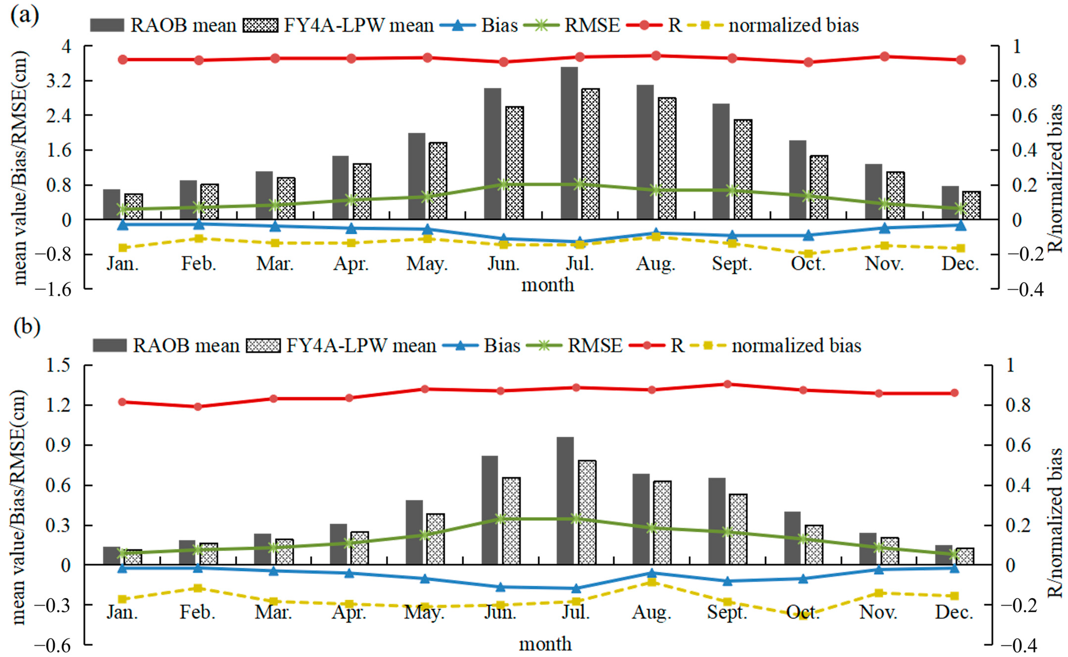
Figure 4 shows the statistical results of various evaluation indicators from January to December from 2019 to 2020. As shown in Figure 4, the evaluation indicators of FY-4A/AGRI LPW in the whole layer, high layer, middle layer, and low layer demonstrated the same characteristics; the mean values of FY-4A/AGRI LPW in various months were all lower than those of RAOB TPW, indicating the underestimations of FY-4A/AGRI LPW in various months. The R remained at a relatively high level and demonstrated satisfactory stability along with changes in time. The Bias and RMSE were relatively high in June and July, while they were relatively low in other months. Considering that LPW values in June and July were relatively larger, we normalized Bias (Bias/FY-4A-LPW mean) to further analysis FY-4A/AGRI LPW quality.

Figure 4a shows a comparison of the whole-layer water vapor values of FY-4A/AGRI LPW and RAOB TPW. It can be seen in the figure that the mean values of water vapor of FY-4A/AGRI LPW and RAOB TPW were highest in June, July, and August, then decreased progressively toward two sides. The mean values were lowest in January, February, and December, which conformed to the actual change rule of the atmospheric water vapor in the Southeastern Tibetan Plateau along with changes in months. In terms of correlation, a high correlation was maintained in various months in these two years, and the change in the correlation along with the time was relatively stable. Both the Bias and RMSE were highest in June, July, and August, and lowest in January and December. The normalized Bias of each month was relatively stable.

As shown in Figure 4b, the variation of these two kinds of water vapor value was similar to the whole layer. The R of high layer had reached a level above 0.8. In comparison with the whole layer, the stability was poorer relatively, and the values in January and February were relatively low. The Bias was highest in June and July, and lowest in January and December. Different from the water vapor in the whole layer, the deviation of FY-4A/AGRI LPW in the high layer in August was relatively small, and the deviation saw an increase in September. The trend of the RMSE was consistent with that of the whole layer of the water vapor; it was highest in June, July, and August, and lowest in January and December. The normalized Bias was smallest in August and was largest in October.

Figure 4c shows a comparison of the middle-layer water vapor values of FY-4A/AGRI LPW and RAOB TPW. The R was lowest in June, at 0.81. In all other months, it reached a level above 0.85. The mean values of the water vapor and change trend in the whole layer of these two kinds of data were similar. The Bias was highest in June and July, then decreased in August. The deviation in September and October increased again, then decreased to the lowest level in December, January, and February. The RMSE was highest in June, July, and August, and lowest in January and December. Different with Bias, the normalization Bias had an insignificant change in all the months.

Figure 4d shows a comparison of the low-layer water vapor values of FY-4A/AGRI LPW and RAOB TPW. As shown in the figure, the mean values of the water vapor of these two kinds of data were similar to those of the whole layer of the atmospheric air. The R, which remained above 0.9, was the highest and most stable compared to the other layers. The maximum R was as high as 0.95, indicating the best stability of the water vapor in the low layer along with changes of months. The Bias was highest in June and July, and lowest in January and December. The trend of the RMSE was consistent with that of the whole layer of the water vapor; it was highest in June, July, and August, and lowest in January and December. However, the trend of normalization Bias tends to be lager in January and December. Moreover, the Bias and RMSE were the most stable compared to the water vapor of the other layers, indicating that the low layer FY-4A/AGRI LPW was the most stable in precision from the dimension of months.

3.3. The Precision of FY-4A/AGRI LPW in Spatial Distribution

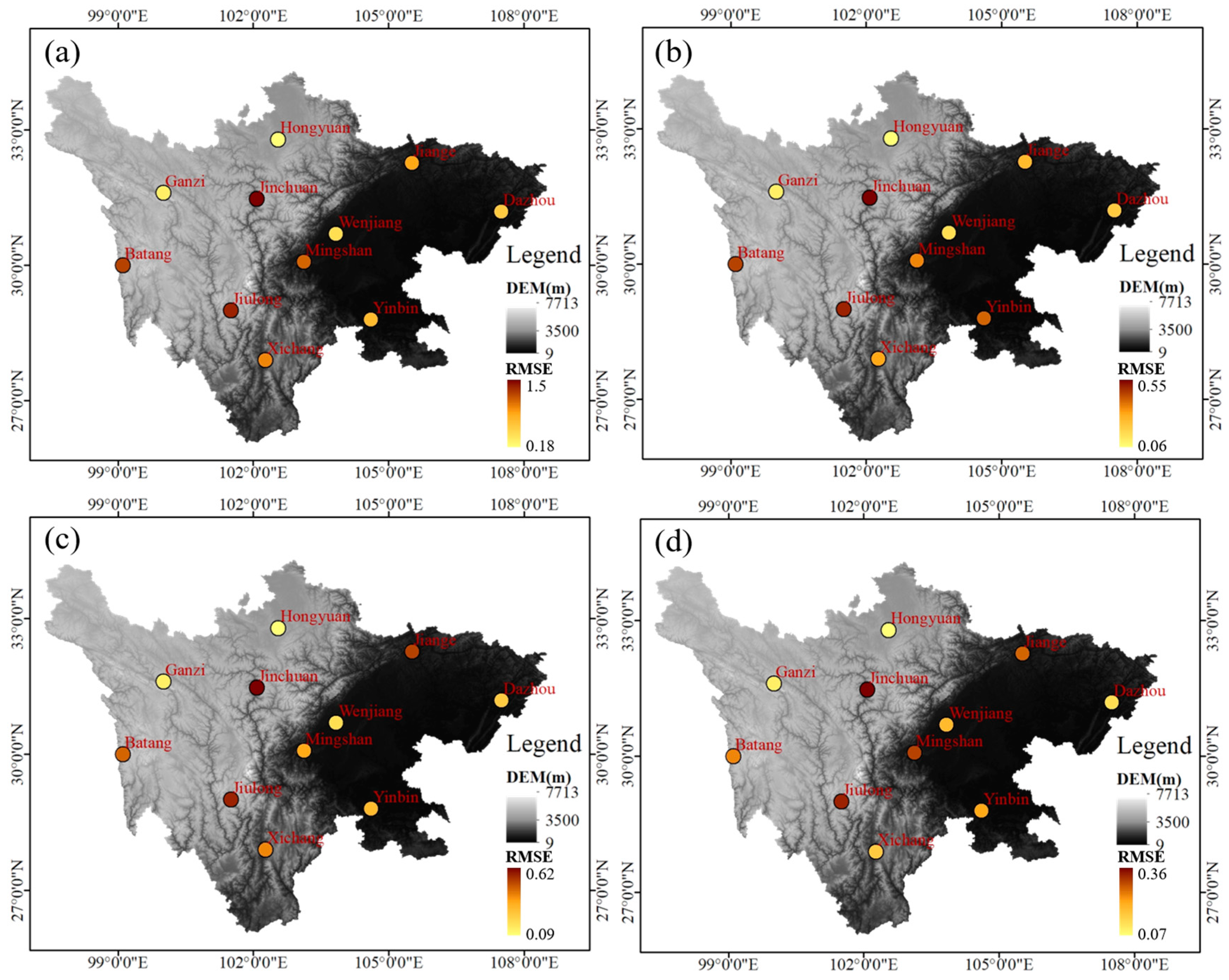
The above discussions indicate the high and stable quality of FY-4A/AGRI LPW in monthly variation. Thus, the following discussions focus on the spatial distribution of FY-4A LPW. Figure 5 shows the spatial patterns of Bias of FY-4A/AGRI LPW from each layer. A relatively large negative Bias at all the layers could be seen over the Jinchuan, Jiulong, and Batang station. While some smaller Bias were found over the north and east of the study area. Similar to the pattern of Bias, the relatively larger RMSE also could be seen over the Jinchuan, Jiulong, and Batang station in Figure 6. The RMSE over Hongyuan and Ganzi station were relatively smaller.

3.3.1. The Correlation between the Precision of FY-4A/AGRI LPW and DEM

As analyzed previously, the terrains of the Southeastern Tibetan Plateau are complex and changeable. In order to study the influence of the altitudes in the research area to the precision of FY-4A/AGRI LPW, we drafted a spatial distribution chart of the Bias and RMSE with respect to the altitude data. The resolution of the datasets of Aster GDEM Version3 digital elevation model (DEM) is 30 m. As shown in Figure 5, the terrains of the research area are high in the west and low in the east, tilting from the northwest to southeast. The maximum DEM difference could be above 7000 m. The eastern part includes a basin with flat terrain and a relatively low DEM. The DEM of the plateau in the western part is mostly above 4000 m. The positions of 11 RAOB stations have significant difference in altitudes, and the precision of FY-4A/AGRI LPW shows obvious differences in spatial distribution.

Figure 5 show that all layers of FY-4A/AGRI LPW have relatively significant underestimate for the central position (eastern of the plateau), and relatively small underestimate in the plain and northwestern region. While FY-4A/AGRI LPW generally underestimated the water vapor content in the whole research area, the Yibin station in the plain overestimated the water vapor. The Bias values of FY-4A/AGRI LPW in the plain area and its surrounding areas, including Wenjiang, Mingshan, Yibin, and Dazhou, were obviously lower than those in stations on the plateau, including Jinchuan, Jiulong, Batang, and Xichang. However, the Bias values of the FY-4A/AGRI LPW data in high-altitude regions, such as Ganzi and Hongyuan station, were relatively small.

In order to perform further quantitative analysis on the relationship between Bias and DEM, a broken line chart for the DEM and the Bias in various layers is shown in Figure 6. The 11 stations show relatively significant differences in DEM values. The one with the highest DEM is Hongyuan Station (3422 m), and the one with the lowest DEM is Dazhou Station (311 m). Although the Jinchuan and Jiulong Stations with a relatively high DEM were obviously underestimated, the Bias of FY-4A/AGRI LPW of Hongyuan Station in various layers, the station with the highest DEM, was relatively small.

Figure 7 shows the spatial distribution layout of RMSE and DEM. The RMSE indicates the dispersion degree among the data. The RMSE over low-altitudes tend to be smaller, and tend to be lager over high-altitudes. Similar to the patterns of Bias, the RMSE of Ganzi and Hongyuan station which in high-altitudes were relatively small.

Figure 8 shows a broken line chart of the RMSE and DEM on the basis of quantitative statistics. It can be seen in the figure that the RMSE values of FY-4A/AGRI LPW in various layers had little relation to the DEM, which is consistent with the Bias results above.

3.3.2. The Correlation between the Precision of FY-4A/AGRI LPW and Relief Degree of Land Surface

The Relief Degree of Land Surface (RDLS) applies the changes in altitude in a certain area to indicate the relief status of the land surface. It is a quantitative basis for the classification of the categories of the topography and landforms [40,41,42]. The FY-4A/AGRI LPW needs to take underlying surface parameters as a background field to retrieve the water vapor information. The RDLS will influence the accuracy and reliability of the values of water vapor retrieved by FY-4A. The significant altitude difference of the junction between the Tibetan Plateau and the Sichuan Basin contribute to the complex and changeable landforms of the research area. Therefore, this study employs the RDLS to discuss its influence on the precision of the FY-4A/AGRI LPW product.

The RDLS can be calculated from the DEM data. The precision of the relief degree will not only be influenced by the spatial resolution of the DEM data and the topographic and geomorphic features of the research area [43], but also rely on the size of the analysis window extract [44]. Based on the datasets of DEM (spatial resolution is 30 m), the best analysis window of RDLS model in this study area were determined by using the mean change point analysis method [45,46]. After multiple experiments, the size of the RDLS model was set to 39 × 39. The RDLS is the altitude difference between the highest and lowest points in a certain region, i.e., the relief features of the land surface within a certain region. The RDLS in the area can be calculated with the following formula:

RDLSi = Max (Hi) − Min (Hi)

(6)

where Hi represents the altitude (m) in the area, and Min (Hi) and Max (Hi) represent the minimum and maximum altitude in the area, respectively.

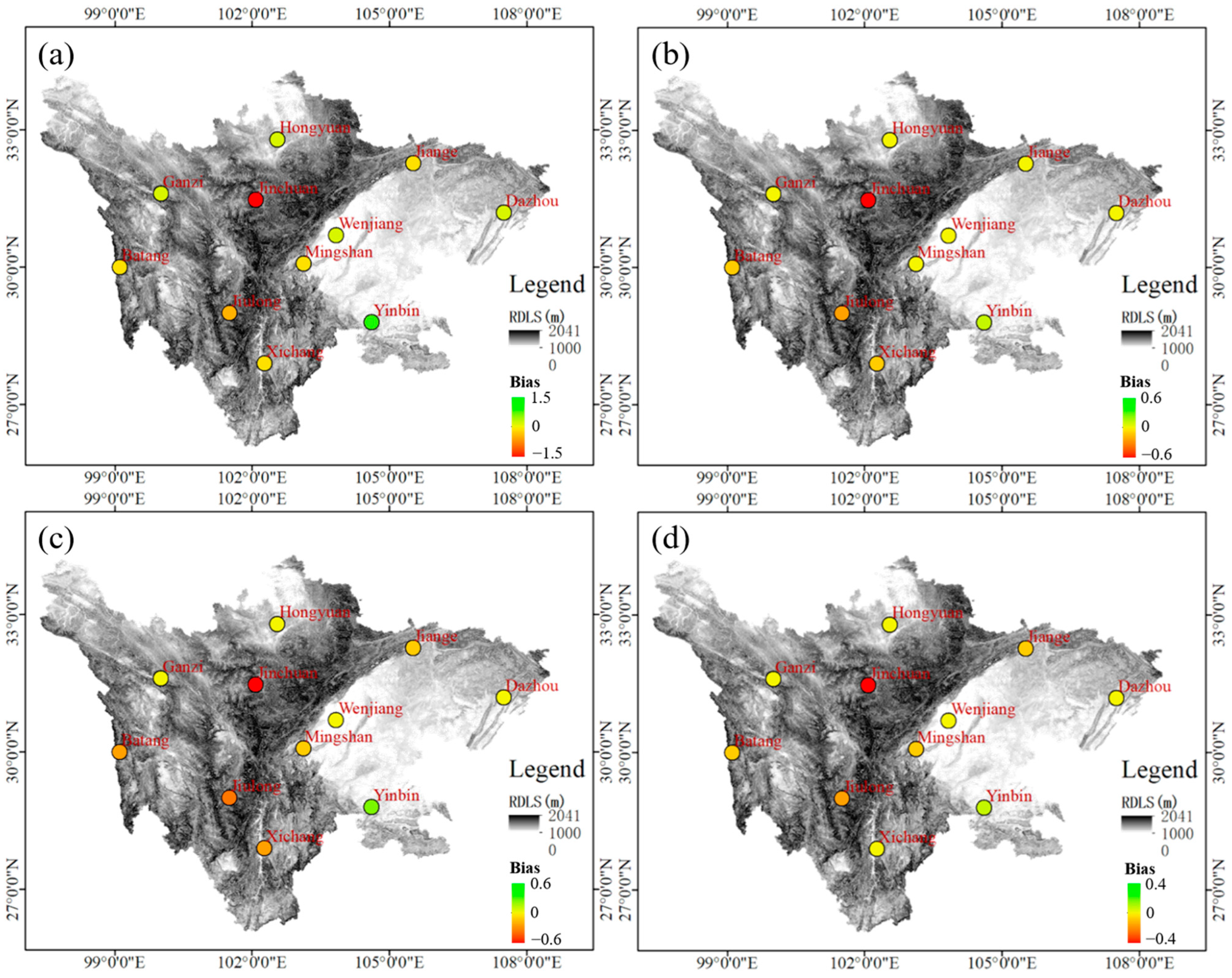
Figure 9 shows the overall spatial distribution between the Bias in the space of various stations and the RDLS. The RDLS of the research area is from 0 m to 2041 m. The 11 stations show significant differences in terrains. Wenjiang, Yibin, and Dazhou in the plain area have a relatively low RDLS, and their Bias’ are relatively small, respectively. Jinchuan, Jiulong, Batang, and other stations on the plateau have a relatively high RDLS, and their Bias’ are relatively large. Notwithstanding the relatively high altitude, the Bias values in Hongyuan and Ganzi were relatively small due to the small RDLS. In terms of analysis from the spatial layout, the Bias had a positive correlation with the RDLS.

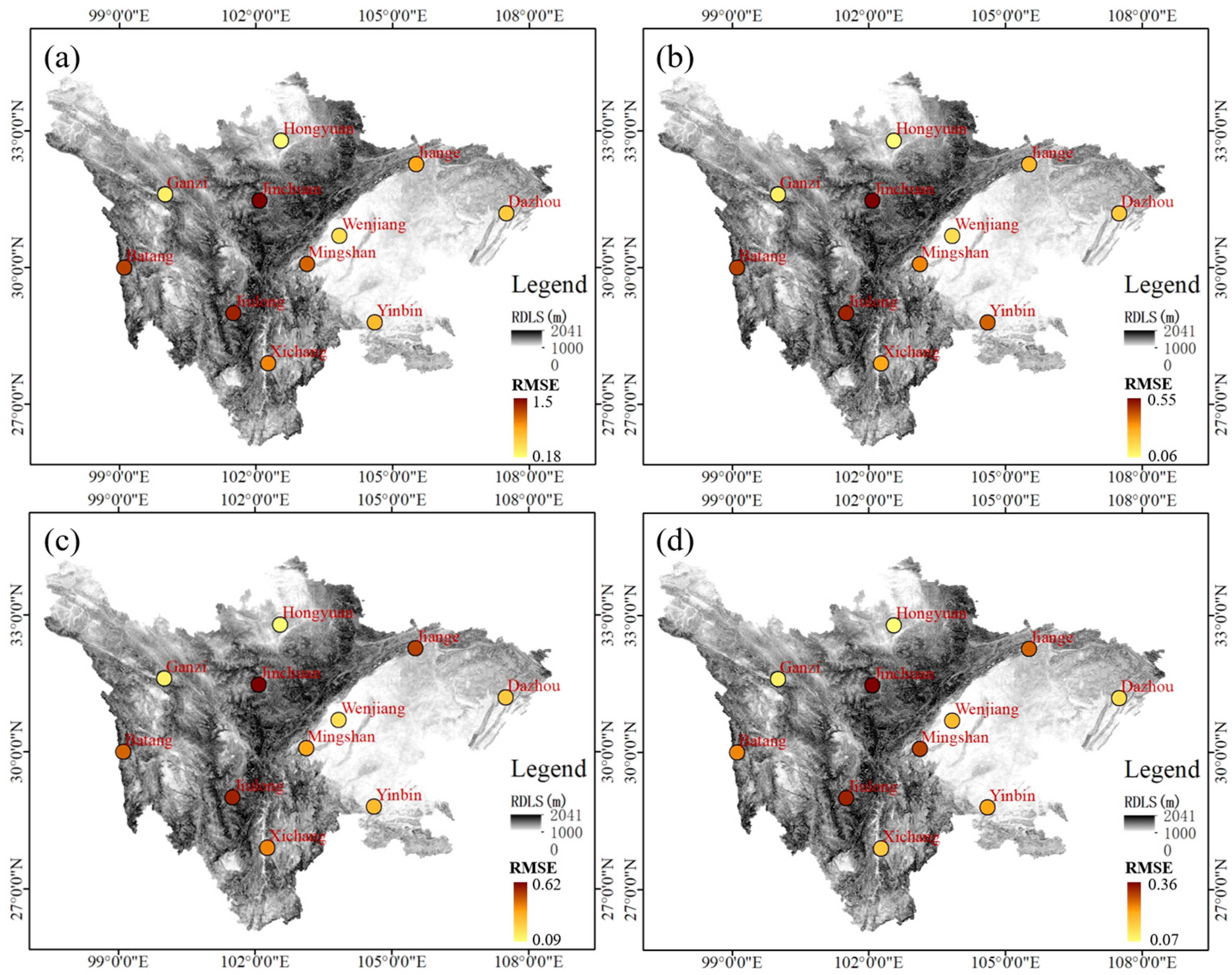
Figure 10 shows the spatial distribution layout of the RMSE and RDLS. Areas with a relatively low RDLS, such as Wenjiang, Dazhou, Hongyuan, and Ganzi, had a relatively small RMSE. Areas with a relatively high RDLS, such as Jinchuan, Jiulong, and Batang, had a relatively large RMSE. Stations at the junction position between the mountainous region and the basin, such as Jiange, Mingshan, and Yibin, showed inconsistent RMSE values of FY-4A/AGRI LPW in various layers. The results demonstrated that the complexity of the landforms will influence the dispersion degree of the data of FY-4A/AGRI LPW product and radiosonde observation to a certain degree. However, the influences at different levels were not consistent with each other.

The above discussions indicate that the precision of FY-4A/AGRI LPW was related with RDLS. Thus, the R between the absolute value of Bias(Abias), RMSE, and the RDLS of each layer were calculated, respectively. It can be seen from

Table 2. The R, slope, and intercept between Abias, RMSE, and RDLS.

Layers	R	Slope	Intercept
Abias-whole (cm)	0.60 *	0.0016	0.2153
Abias-High (cm)	0.35	0.0004	0.1198
Abias-Middle (cm)	0.66 **	0.0006	0.0992
Abias-Low (cm)	0.71 **	0.0004	0.2650
RMSE-Whole (cm)	0.54 *	0.0012	0.4308
RMSE-High (cm)	0.27	0.0003	0.0704
RMSE-Middle (cm)	0.64 **	0.0005	0.1913
RMSE-Low (cm)	0.55 *	0.0002	0.1376

* Means it passed the 90% confidence test; ** means it passed the 95% confidence test.

, the R between Abias and RDLS of the middle layer and low layer were about 0.66–0.71, passed the 95% confidence test. The R between RMSE and RDLS of the middle layer and low layer passed the 95% and 90% confidence test, respectively. The slopes and intercepts showed that the deviation between FY-4A/AGRI LPW and RAOB TPW was positively correlated with RDLS.

4. Conclusions and Discussion

RAOB TPW, recorded at 11 stations on the Southeastern Tibetan Plateau in the period from January 2019 to December 2020, were extracted from the RAOB data, and Bias, RMSE, and R were used to evaluate the FY-4A/AGRI LPW product. The precision and error characteristics of FY-4A/AGRI LPW were summarized and analyzed in terms of vertical height layers, time changes, and spatial distribution. The following conclusions can be drawn.

FY-4A/AGRI LPW and RAOB TPW demonstrate excellent consistency in all of the vertical height layers, but FY-4A/AGRI LPW underestimates precipitable water vapor in southeastern Tibetan Plateau. The correlation coefficient between FY-4A/AGRI LPW and RAOB TPW in high layer was the smallest and the low layer had the best correlation with the RAOB TPW. The Bias and RMSE in middle layer were the biggest. The mean values of FY-4A/AGRI LPW in various months were all lower than those of RAOB TPW, indicating the underestimations of FY-4A/AGRI LPW in various months. The mean values of water vapor of FY-4A/AGRI LPW and RAOB TPW were highest in June, July, and August, then decreased progressively toward two sides. The mean values were lowest in January, February, and December, which conformed to the actual change rule of the atmospheric water vapor in the Southeastern Tibetan Plateau along with changes in months. The Bias and RMSE of the low-layer were the most stable compared to other layers, indicating that the low layer FY-4A/AGRI LPW was the most stable in precision from the dimension of months.

The precision of FY-4A/AGRI LPW was related with RDLS, and the deviation between FY-4A/AGRI LPW and RAOB TPW was positively correlated with RDLS. The complexity of the landforms will influence the dispersion degree of the data of FY-4A/AGRI LPW product and radiosonde observation to a certain degree. However, the influences at different levels were not consistent with each other.

Inspit of the overall dry bias in Southeastern Tibetan Plateau, the FY-4A/AGRI LPW FY-4A/AGRI LPW had a relatively high precision, and the data from it had superior quality and stability in terms of time changes and spatial distribution. Therefore, the product can perfectly reflect the spatial and temporal variation of the atmospheric water vapor on the Southeastern Tibetan Plateau. Combined with the description of algorithm for FY-4A/AGRI LPW by Zhang Yong et al. [37], there are two factors that can explain the deviations between the FY-4A/AGRI LPW and RAOB TPW. They are: (1) the matching processing of FY-4A/AGRI LPW and RAOB; (2) the uncertainties in the surface infrared emissivity. In this study, the three-dimensional Matching was used to minimize the deviations of FY-4A/AGRI LPW and RAOB TPW. However, the uncertainties of the drift distance of sounding balloons may also affect the comparison, especially to the high layer. That may explain the least correlation in high layer. In addition, Surface emissivity is an important parameter of the algorithm for FY-4A/AGRI LPW. Topographic relief will lead to the errors of surface emissivity. Thus, the surface emissivity could be an important factor in the deviations of middle and low layers between FY-4A/AGRI LPW and RAOB TPW in the larger RDLS region.

References

1. Wu, M.; Jin, S.; Li, Z.; Cao, Y.; Ping, F. High-Precision GNSS PWV and Its Variation Characteristics in China Based on Individual Station Meteorological Data. Remote Sens. 2021, 13, 1296. [Google Scholar] [CrossRef]
2. Gilmore, J.B. Understanding the Influence of Measurement Uncertainty on the Atmospheric Transition in Rainfall and Column Water Vapor. J. Atmos. Sci. 2015, 72, 2041–2054. [Google Scholar] [CrossRef]
3. Hu, P.; Wang, M.; Yang, L.; Wang, X.; Feng, G. Water Vapor Transport Related to the Interdecadal Shift of Summer Precipitation over Northern East Asia in the Late 1990s. J. Meteorol. Res. 2018, 32, 113–125. [Google Scholar] [CrossRef]
4. Miranda, P.; Mateus, P. A new unconstrained approach to GNSS atmospheric water vapor tomography. Geophys. Res. Lett. 2021, 48, ee2021GL094852. [Google Scholar] [CrossRef]
5. Trenberth, K.; Smith, L.; Qian, T.; Dai, A.; Fasullo, J. Estimates of the Global Water Budget and Its Annual Cycle Using Observational and Model Data. J. Hydrometeorol. 2007, 8, 758–769. [Google Scholar] [CrossRef] [Green Version]
6. Feng, X.; Yan, H.; Wang, S.; Qiu, G.; Tang, S.; Shang, L.; Dai, Q.; Hou, Y. Seasonal variation of gaseous mercury exchange rate between air and water surface over Baihua reservoir, Guizhou, China. Atmos. Environ. 2004, 38, 4721–4732. [Google Scholar] [CrossRef]
7. He, Q.; Shen, Z.; Wan, M.; Wan, M.; Li, L. Perceptible Water Vapor Converted from GNSS-ZTD and ERA5 Datasets for the Monitoring of Tropical Cyclones. IEEE Access 2020, 8, 87275–87290. [Google Scholar] [CrossRef]
8. Solomon, S.; Rosenlof, K.; Portmann, R.; Daniel, J.; Davis, S.; Sanford, T.; Plattner, G. Contributions of stratospheric water vapor to decadal changes in the rate of global warming. Science 2010, 5970, 1219–1223. [Google Scholar] [CrossRef] [Green Version]
9. Wagner, T.; Beirle, S.; Grzegorski, M.; Platt, U. Global trends (1996–2003) of total column precipitable water observed by Global Ozone Monitoring Experiment (GOME) on ERS-2 and their relation to near-surface temperature. J. Geophys. Res. 2006, 111, 2193–2214. [Google Scholar] [CrossRef] [Green Version]
10. Trenberth, K.; Fasullo, J.; Smith, L. Trends and variability in column-integrated atmospheric water vapor. Clim. Dyn. 2005, 24, 741–758. [Google Scholar] [CrossRef]
11. Shoji, Y.; Sato, K.; Yabuki, M.; Tsuda, T. Comparison of shipborne GNSS-derived perceptible water vapor with radiosonde in the western North Pacific and in the seas adjacent to Japan. Earth Planets Space 2017, 69, 153. [Google Scholar] [CrossRef]
12. He, W.; Cheng, Y.; Zou, R.; Wang, P.; Chen, H.; Li, J.; Xia, X. Radiative Transfer Model Simulations for Ground-Based Microwave Radiometers in North China. Remote Sens. 2021, 13, 5161. [Google Scholar] [CrossRef]
13. Sun, W.; Wang, J.; Li, Y.; Meng, J.; Zhao, Y.; Wu, P. New Gridded Product for the Total Columnar Atmospheric Water Vapor over Ocean Surface Constructed from Microwave Radiometer Satellite Data. Remote Sens. 2021, 13, 2402. [Google Scholar] [CrossRef]
14. Bai, T.; Ding, J.; Liu, Y.; Wu, Y. Application of Microwave Radiometer in Monitoring Water Vapor Characteristics and Precipitation Analysis. Meteorol. Environ. Sci. 2021, 44, 102–107. [Google Scholar]
15. Wu, Z.; Liu, Y.; Liu, Y.; Wang, J.; He, X.; Xu, W.; Ge, M.; Schuh, H. Validating HY-2A CMR precipitable water vapor using ground-based and shipborne GNSS observations. Atmos. Meas. Tech. 2020, 13, 4963–4972. [Google Scholar] [CrossRef]
16. Van, M.; Rorland, P.; Pottiaux, E.; Stankunavicius, G.; Beirle, S.; Wagner, T.; Brenot, H.; Bruyninx, C.; Jones, J. Global Spatiotemporal Variability of Integrated Water Vapor Derived from GPS, GOME/SCIAMACHY and ERA-Interim: Annual Cycle, Frequency Distribution and Linear Trends. Remote Sens. 2022, 14, 1050. [Google Scholar] [CrossRef]
17. Lu, C.; Chen, X.; Liu, G.; Galina, D.; Jens, W.; Jiang, X.; Zheng, K.; Harald, S. Real-Time Tropospheric Delays Retrieved from Multi-GNSS Observations and IGS Real-Time Product Streams. Remote Sens. 2017, 9, 1317. [Google Scholar] [CrossRef] [Green Version]
18. Xiong, Z.; Sun, X.; Sang, J.; Wei, X. Modify the Accuracy of MODIS PWV in China: A Performance Comparison Using Random Forest, Generalized Regression Neural Network and Back-Propagation Neural Network. Remote Sens. 2021, 13, 2215. [Google Scholar] [CrossRef]
19. Li, X.; Tan, H.; Li, X. Real-Time Sensing of Precipitable Water Vapor from BeiDou Observations: Hong Kong and CMONOC Networks. J. Geophys. Res. Atmos. 2018, 123, 7897–7909. [Google Scholar] [CrossRef] [Green Version]
20. Nelson, R.R.; Crisp, D.; Ott, L.E.; O’Dell, C.W. High-accuracy measurements of total column water vapor from the orbiting carbon observatory-2. Geophys. Res. Lett. 2016, 43, 12261–12269. [Google Scholar] [CrossRef] [Green Version]
21. Cao, X.; Li, X.; Liu, S.; Zhang, X. Assessment of Spectra of the Atmospheric Infrared Ultraspectral Sounder on GF-5 and Validation of Water Vapor Retrieval. Sensors 2021, 21, 325. [Google Scholar] [CrossRef]
22. He, J.; Liu, Z. Water vapor retrieval from MERSI NIR channels of Fengyun-3B satellite using ground-based GPS data. Remote Sens. Environ. 2021, 258, 112384. [Google Scholar] [CrossRef]
23. Niell, A.; Coster, A.; Solheim, F.; Mendes, V.; Toor, P.; Langley, R.; Upham, C. Comparison of measurements of atmospheric wet delay by radiosonde, water vapor radiometer, GPS, and VLBI. J. Atmos. Ocean. Technol. 2001, 18, 830–850. [Google Scholar] [CrossRef]
24. Adeyemi, B.; Joerg, S. Analysis of water vapor over Nigeria using radiosonde and satellite data. J. Appl. Meteorol. Climatol. 2012, 51, 855–1866. [Google Scholar] [CrossRef]
25. Seemann, S.; Li, J.; Menzel, W.; Gumley, L. Operational retrieval of atmospheric temperature, moisture, and ozone from MODIS infrared radiances. J. Appl. Meteorol. 2003, 42, 1072–1091. [Google Scholar] [CrossRef]
26. King, M.; Kaufman, Y.; Menzel, W.; Tanre, D. Remote sensing of cloud, aerosol, and water vapor properties from the moderate resolution imaging spectrometer (MODIS). IEEE Trans. Geosci. Remote Sens. 1992, 30, 2–27. [Google Scholar] [CrossRef] [Green Version]
27. Kaufman, Y.; Gao, B. Remote sensing of water vapor in the near IR from EOS/MODIS. IEEE Trans. Geosci. Remote Sens. 1992, 30, 871–884. [Google Scholar] [CrossRef]
28. Yang, J.; Zhang, Z.; Wei, C.; Lu, F.; Guo, Q. Introducing the new generation of Chinese geostationary weather satellites, FENGYUN-4. Bull. Am. Meteorol. Soc. 2016, 98, 1637–1658. [Google Scholar] [CrossRef]
29. Zhang, X.; Xu, D.; Liu, R.; Shen, F. Impacts of FY-4A AGRI Radiance Data Assimilation on the Forecast of the Super Typhoon “In-Fa” (2021). Remote Sens. 2022, 14, 4718. [Google Scholar] [CrossRef]
30. Niu, Z.; Zhang, L.; Dong, P.; Weng, F.; Huang, W.; Zhu, J. Effects of Direct Assimilation of FY-4A AGRI Water Vapor Channels on the Meiyu Heavy-Rainfall Quantitative Precipitation Forecasts. Remote Sens. 2022, 14, 3483. [Google Scholar] [CrossRef]
31. Ren, J.; Xu, G.; Zhang, W.; Leng, L.; Xiao, Y.; Wan, R.; Wang, J. Evaluation and Improvement of FY-4A AGRI Quantitative Precipitation Estimation for Summer Precipitation over Complex Topography of Western China. Remote Sens. 2021, 13, 4366. [Google Scholar] [CrossRef]
32. Wu, G.; Liu, Y.; He, B.; Bao, Q.; Duan, A.; Jin, F. Thermal controls on the Asian summer monsoon. Sci. Rep. 2012, 2, 404. [Google Scholar] [CrossRef] [Green Version]
33. Rajagopalan, B.; Molnar, P. Signatures of Tibetan Plateau heating on Indian summer monsoon rainfall variability. J. Geophys. Res. 2013, 118, 1170–1178. [Google Scholar] [CrossRef]
34. Xu, X.; Lu, C.; Ding, Y.; Shi, X.; Guo, Y.; Zhu, W. What is the relationship between China summer precipitation and the change of apparent heat source over the Tibetan Plateau? Atmos. Sci. Lett. 2013, 14, 227–234. [Google Scholar] [CrossRef]
35. Li, Y.; Li, D.; Yang, S.; Liu, C.; Zhong, A.; Li, Y. Characteristics of the precipitation over the eastern edge of the Tibetan Plateau. Meteorol. Atmos. Phys. 2010, 106, 49–56. [Google Scholar] [CrossRef]
36. Wang, Y.; Wang, L.; Li, X.; Chen, D. Temporal and spatial changes in estimated near-surface air temperature lapse rates on Tibetan Plateau. Int. J. Climatol. 2018, 38, 2907–2921. [Google Scholar] [CrossRef] [Green Version]
37. Zhang, Y.; Li, Z.; Jun, L. A preliminary layer perceptible water vapor retrieval algorithm for FengYun-4 advanced geosynchronous radiation imager. In Proceedings of the IGARSS 2019—2019 IEEE International Geoscience and Remote Sensing Symposium, Yokohama, Japan, 28 July–2 August 2019; pp. 7564–7566. [Google Scholar]
38. Heng, Z.; Jiang, X. An Assessment of the Temperature and Humidity of Atmospheric Infrared Sounder (AIRS) v6 Profiles Using Radiosonde Data in the Lee of the Tibetan Plateau. Atmosphere 2019, 10, 394. [Google Scholar] [CrossRef] [Green Version]
39. Zhang, Y.; Li, J.; Li, Z.; Zheng, J.; Wu, D.; Zhao, H. FENGYUN-4A Advanced Geosynchronous Radiation Imager Layered Precipitable Water Vapor Products’ Comprehensive Evaluation Based on Quality Control System. Atmosphere 2022, 13, 290. [Google Scholar] [CrossRef]
40. Feng, Z.; Li, W.; Li, P.; Xiao, C. Relief degree of land surface and its geographical meanings in the qinghai-tibet plateau, China. Acta Geogr. Sin. 2020, 75, 1359–1372. [Google Scholar]
41. Liu, Y.; Deng, W.; Song, X. Relief Degree of Land Surface and Population Distribution of Mountainous Areas in China. J. Mt. Sci. 2015, 2, 518–532. [Google Scholar] [CrossRef]
42. Wang, L.; Liu, X.; Li, D.; Sun, Y. Geographical Detection of Spatial Heterogeneity and Drivers of PM2.5 in the Yangtze River Economic Belt. Environ. Sci. 2022, 43, 1190–1200. [Google Scholar]
43. Cen, Y.; Zhang, B.; Luo, J.; Deng, Q.; Liu, H.; Wang, L. Influence of Topographic Factors on the Characteristics of Gully Systems in Mountainous Areas of Ningnan Dry-Hot Valley, SW China. Int. J. Environ. Res. Public Health 2022, 19, 8748. [Google Scholar] [CrossRef] [PubMed]
44. Zhang, X.; Dong, K. Neighborhood Analysis-Based Calculation and Analysis of Multi-Scales Relief Amplitude. Adv. Mater. Res. 2012, 468–471, 2086–2089. [Google Scholar] [CrossRef]
45. Chen, X.; Zhang, X.; Chang, Q. A study on Optimal Statistical Unit of Relief Amplitude of Land Surface in Shaanxi Province. Bull. Soil Water Conserv. 2016, 36, 265–270+370. [Google Scholar]
46. Zhang, W.; Li, A. Study on the Optimal Scale for Calculating the Relief Amplitude in China Based on DEM. Geogr. Geo-Inf. Sci. 2012, 28, 8–12. [Google Scholar]
Figure 1. The topography and distribution of RAOB stations in the study region.
Atmosphere 14 00277 g001
Figure 2. Scatter plot between FY-4A/AGRI LPW and RAOB TPW. (a) Whole layer; (b) high layer; (c) middle layer; (d) low layer.
Atmosphere 14 00277 g002
Figure 3. The histograms of the Bias. (a) Whole layer; (b) high layer; (c) middle layer; (d) low layer.
Atmosphere 14 00277 g003
Figure 4. Monthly time series of the Bias and RMSE. (a) Whole layer; (b) high layer; (c) middle layer; (d) low layer.
Atmosphere 14 00277 g004aAtmosphere 14 00277 g004b
Figure 5. Spatial distribution of Bias and DEM. (a) Whole layer; (b) high layer; (c) middle layer; (d) low layer.
Atmosphere 14 00277 g005
Figure 6. Statistics of the Bias and DEM from each RAOB station.
Atmosphere 14 00277 g006
Figure 7. Spatial distribution of RMSE and DEM. (a) Whole layer; (b) high layer; (c) middle layer; (d) low layer.
Atmosphere 14 00277 g007
Figure 8. Statistics of the RMSE and DEM from each RAOB station.
Atmosphere 14 00277 g008
Figure 9. Spatial distribution of Bias and RDLS. (a) Whole layer; (b) high layer; (c) middle layer; (d) low layer.
Atmosphere 14 00277 g009
Figure 10. Spatial distribution of the RMSE and RDLS. (a) Whole layer; (b) high layer; (c) middle layer; (d) low layer.
Atmosphere 14 00277 g010