Simulation of the Spatial Flow of Wind Erosion Prevention Services in Arid Inland River Basins: A Case Study of Shiyang River Basin, NW China

Abstract

Wind erosion is a key global environmental problem. As an important protective measure to provide services to the ecosystems in wind-eroded areas, the wind erosion prevention service is of great significance to the management of wind and sand hazards and ecological environment restoration in the wind-eroded areas and the neighboring areas. Taking the Shiyang River basin as the study area, the quality of supplies for wind erosion prevention services was estimated using the RWEQ model for the years 2005, 2010, 2015, and 2020; the trajectories of air masses at wind speeds higher than the sand-causing wind speeds were simulated based on the forward trajectory module of the HYSPLIT model for a 24 h period; the spatial simulation of the flow of wind erosion prevention services on a daily scale with Minqin Station as the sand source was carried out; and the beneficiary areas of wind erosion prevention services were identified. Based on the RWEQ model, the spatial patterns of potential wind erosion, actual wind erosion, and wind and sand stabilization services were obtained, and the supply areas were divided. From 2005 to 2020, the wind erosion prevention service flow in the Shiyang River basin was distributed along a northwest–southeast direction, with a radial decrease from the center to the periphery, and with an extremely strong extraterritorial effect. The amount of wind erosion in the basin has a variable downward tendency over time and a spatial distribution pattern of high in the north and low in the south. The area of higher sand fixation is distributed in the eastern oasis area and desert junction zone. The HYSPLIT model was used to simulate the transport paths of wind and sand within 24 h during 2005–2020, the transmission paths of the wind erosion prevention service flow were obtained to be 59–134, and the flows were 2.55 × 10⁴–3.85 × 10⁶ t, displaying a changing trend of first decreasing, then increasing, and then decreasing. Gansu Province, Ningxia Hui Autonomous Region, and Inner Mongolia Autonomous Region are the most important areas benefiting from the wind erosion prevention service flow in the Shiyang River basin. The wind erosion prevention service flows in the basin benefit 47 cities in 9 provinces.

1. Introduction

The ecosystems of China’s arid inland river basins have been seriously degraded as a result of population growth and inefficient economic development patterns, and the ecosystem services (ESs) provided to humans are decreasing, facing a significant danger to ecological security and a significant obstacle to sustainable development [1,2,3]. Static ecosystem service assessment studies have ignored the flow of ESs caused by the imbalance in supply and benefit regions’ spatial distribution, reducing the guiding role of ESs in ecological protection and construction. ES flow establishes a spatial and temporal link between the supplying and benefiting ends [4,5,6] and plays a significant part in the formation, transport, modification, and upkeep of ESs. Quantitative study of ESs is conducive to systematically revealing the process of ES transfer, which helps to spatially and accurately assess the actual ESs and is crucial to the execution of policies for ecosystem management, such as ecosystem protection and ecological compensation. The transitional landscape of mountain–oasis–desert is a typical ecological feature of arid inland river basins, which creates substantial spatial heterogeneity in the basin’s supply and benefit as well as strong mobility of ESs.

Soil wind erosion (WE) is one of the major causes of land degradation globally [7,8,9]. Dust storms and strong winds are frequent as a result of global warming, and soil WE has become more severe in various regions [10,11]. Northwest China is part of the central Asian dust storm-prone area, and one of the most significant ecological issues in the dry and semiarid regions of northern China is sand erosion [12]. The ecological environment that humans depend on for survival is severely harmed by sand and dust storms, and the dust forms a large pollution zone downwind, which directly affects the quality of life of human beings and their production efficiency [13]. In order to alleviate the impact of wind and sand on human beings, it is crucial to clarify the change rule in the spatial location of wind erosion; for this reason, many scholars have utilized field sand collectors, indoor wind tunnels and movable wind tunnels [14,15], isotope tracers, etc., to study wind erosion; all these methods require a lot of manpower, material, and financial resources, and it is very difficult to expand the results of the study on the point scale to the regional scale, but it lays the foundation for the subsequent application of the model. Wind erosion prevention (WEP) services provided by ecosystems refer to the services that ecosystems located in dust source areas that have the effect of reducing wind speed and fixing soil [16,17,18], which can reduce or avoid the harmful effects of sand and dust weather on human beings after soil erosion and affect the ecology of the whole region as well as that of the downwind area.

Currently, the common models used to simulate and quantify wind erosion and sand stabilization services are the wind erosion equation (WEQ) model, Texas erosion and accretion (TEAM) model, wind erosion stochastic simulation (WESS) model, revised wind erosion equation (RWEQ) model, and wind erosion prediction system (WEPS). Although the integrated application of GIS, remote sensing, and model simulation has overcome the shortcomings of field experiments, the limitations of statistical and empirical wind erosion estimation studies have become more and more obvious, and therefore more and more studies have used the RWEQ to quantify WEP services. The RWEQ model is simple in operation and requires little data; so as long as there are ideal input data such as soil and meteorological data, the model can predict wind erosion well, and can estimate soil wind erosion in a long time series at the regional scale, so as to provide a better basis for regional desertification control. As a typical regulating service, WEP services have obvious spatial mobility, and portraying the flow of WEP services from the supply side to the use side spatially is conducive to understanding and clarifying the natural transmission mode of WEP services and the dynamic process of inhibiting wind and sand transmission spatially at the place of sand origin, thus enhancing the capacity of WEP and reducing the harm of sand and dust in the downwind direction. Shiyang River basin (SRB) is surrounded by the Tengger and Badain Jaran deserts to the north, which poses a major danger to the basin’s ecological ecosystem. As a significant component of China’s “Qinghai-Tibet Plateau Ecological Barrier and Northern Sand Control Belt”, the problem of wind and sand is very prominent in the SRB.

The challenge and emphasis of ES research is ES flow, and research in this area is still in the initial development stage. Among them, the exploration of the concept and characteristics of ES flows is still ongoing, while the quantification of ES flows and the identification of complete routeways has become a hotspot of late [19,20,21]. Based on GIS technology, using remote sensing information, depicting ES flow routes through spatially distributed models, and simulating the spatial flow process of ESs are important development directions for ES flow research [22,23,24,25]. Several models have been used by many researchers to study the ES flow process. However, the process of ES transfer is complex, involving the combined impacts of several biotic and abiotic factors, and a vast number of parameters that must be taken into account during model simulation, which makes the simulation of the ES flow transfer process a great challenge. Accurate simulation of ES flows not only improves understanding of ESs in the spatial transmission process and deepens the connotation of ES research, but also has important implications for ecosystem management and ecological compensation and other practical work.

Based on the above reasons, this paper’s study goals are (1) to quantitatively demonstrate the spatial and temporal relationship between the provision of WEP services and their beneficial effects in the SRB, (2) to achieve spatialized modeling of the WEP services’ flow routes and quantitative measurement of the flow, and (3) to explore the characteristics of the spatial and temporal changes in the flow of WEP services in SRB.

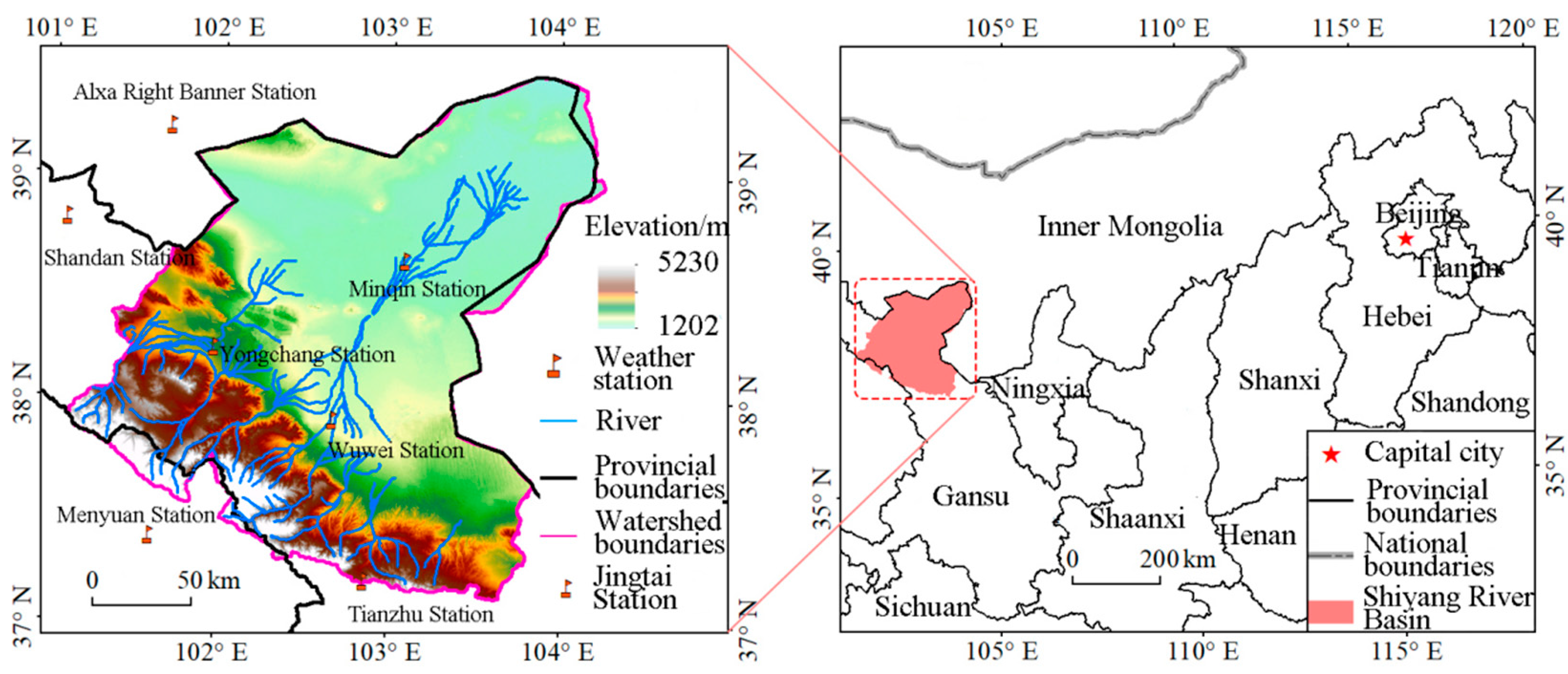
2. Study Area

SRB is a typical inland river in northwest China (Figure 1), with a length of about 250 km, originating from the northern foothills of the Qilian Mountains, and formed by the confluence of eight rivers, including the Xida River and Dongda River. The basin an area of approximately 4.12 × 10⁴ km² and is situated 37°02′–39°17′ N, 100°57′–104°12′ E. It borders the Badain Jaran desert, the Tengger desert, the Qilian Mountains, the Yellow River basin, and Heihe River basin. The basin’s topography is tilted from the southwest to the northeast and is high in the south and low in the north. With a 2–8 °C yearly mean temperature, 50–700 mm of rainfall per year, 700–2600 mm of evaporation per year, the basin experiences a typical temperate continental climate. Alpine grassland and forest ecosystems predominate in the basin’s upper parts, while the temperate arid areas in the middle and lower reaches of the basin are densely populated, with a high concentration of industries and extensive farmland. The total population in the basin is 2.17 million, of which 1.11 million are rural. In 2020, the GDP of the basin will be USD 11.79 billion, of which USD 2.56 billion will be in primary industry, USD 4.23 billion in secondary industry, and USD 5.00 billion in tertiary industry. SRB is a densely populated area in northwest China, with a high degree of water resources exploitation and utilization, prominent water use conflicts, and extremely strong constraints of soil and water resources on socioeconomic development. With the impact of manmade activities and global warming, the ecological environment of the SRB is deteriorating, seriously endangering the survival of its inhabitants.

3. Data and Methodology

3.1. Data Source

Data on land use for the years 2005, 2010, 2015, and 2020 are available from the Chinese Academy of Sciences’ Resource and Environment Data Center (https://www.resdc.cn/AchievementList1.aspx, accessed on 10 August 2023). The Geospatial Data Cloud served as the source for the digital elevation model (DEM) (http://www.ncdc.ac.cn, accessed on 13 August 2023). Data on soil texture were gathered from the Chinese Soil Characteristics Dataset of the National Glacial Tundra Desert Science Data Centre (http://www.iiasa.ac.at/Research/LUC/External-World-soil-database/HTML/, accessed on 10 August 2023), which was compiled based on the 1:1 million soil type map and the second soil census data, and the data were divided into three categories: sand, silt, and clay. Soil depth, rooting depth coefficient, organic matter content, and bulk weight were obtained from the Harmonized World Soil Databases, with a resolution of 1 × 1 km. The annual NDVI data were obtained from the MOD13Q1 product of the National Aeronautics and Space Administration (NASA) (www.nasa.gov/, accessed on 23 August 2023) of the United States of America (USA), and the highest possible value generation technique was used to combine the annual NDVI data. The aforementioned data have a 1 km spatial resolution. Meteorological data were obtained from the China Meteorological Data Sharing Network (http://data.cma.cn/, accessed on 16 August 2023), and to ensure the accuracy of the data, in addition to the four stations inside the study area, the data from nine meteorological stations in the surrounding area were also obtained, and the spatial interpolation was carried out by using ANUSPLIN 4.4 software to obtain the spatialized data of precipitation and evapotranspiration with a spatial resolution of 1 km. The data were spatially interpolated using ANUSPLIN software. The sand transport was obtained from the Gansu Provincial River Sediment Bulletin. All geographic information was converted to the Albers uniform cylindrical projection method in order to maintain the integrity of coordinates and reduce area distortion, and all of the data were processed to a raster with a 1 × 1 km resolution.

3.2. Methodology

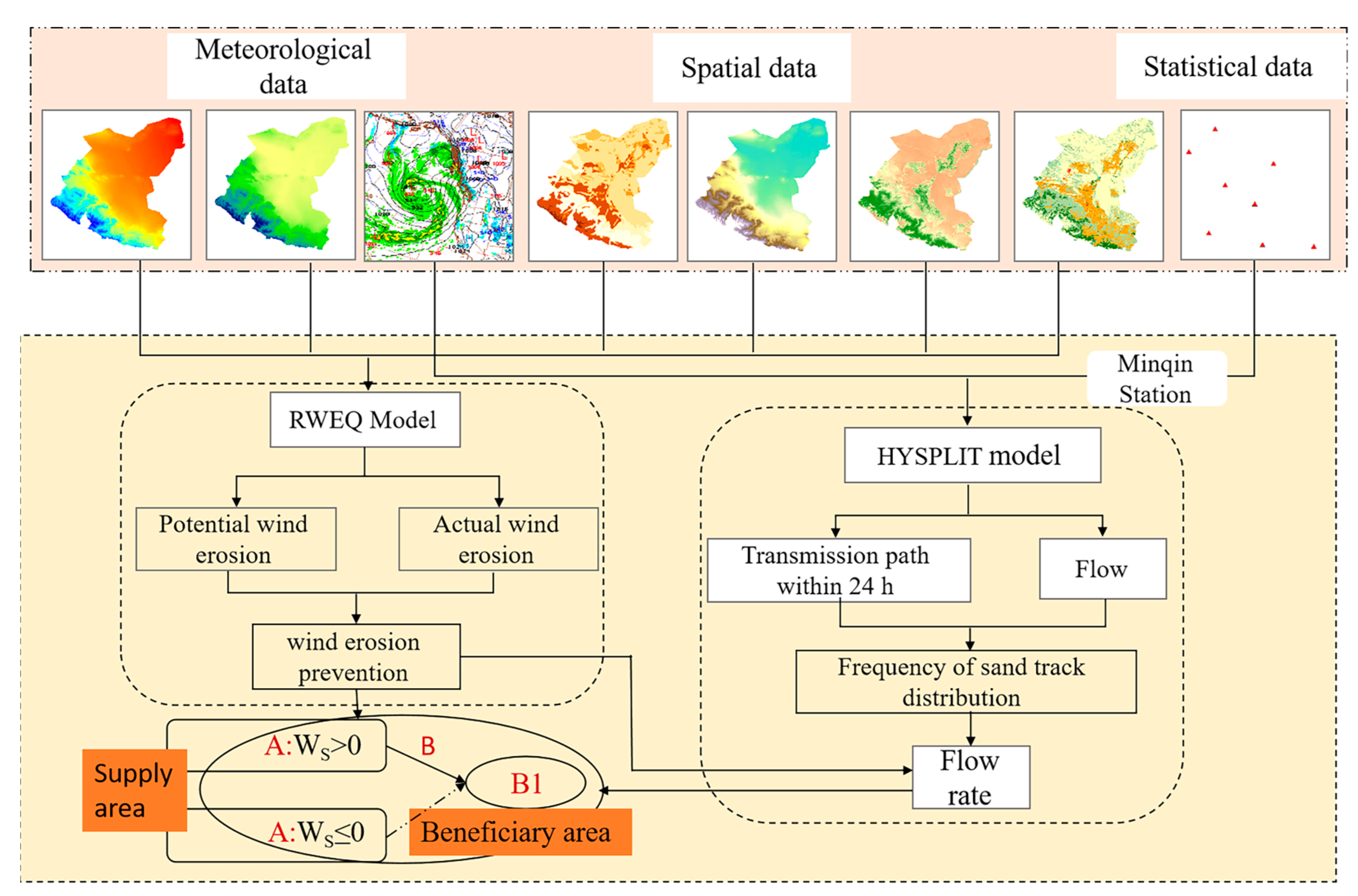
3.2.1. Research Framework

WEP services refer to services in which ecosystem vegetation located in dust and sand source areas has the effect of reducing wind speed and fixing the soil, reducing or avoiding the formation of dust and sandy weather after the soil has been eroded, which hurts human beings [26]. The transport of wind and sand is controlled by air masses, and as the transport capacity of the air mass decreases or the sand and dust carried by it settles, the transport of wind and sand is also cut off, which is the end of the transport path of the WEP service. However, the movement of air masses is extremely complex, and the settling effect along the way is affected by many factors, making it difficult to simulate the inhibition of their transmission. Therefore, the simulation process for the flow of WEP services is simplified, without considering the settlement and interception along the way; the transmission starts with a wind speed more than the sand initiation speed (>5 m·s⁻¹) at the sand source, and this paper only simulates the transmission route within 24 h. The benefits provided by WEP services mainly for human beings include services to reduce topsoil loss, protect soil fertility, and mitigate sedimentation, but the two capacities of reducing topsoil loss and protecting soil fertility, which are specific to the place where WE occurs, their flows are in situ, and no spatial transport occurs. Eroded wind sand may either stay in place or move downwind, and its flow belongs to allostatic flow due to the variable and unstable wind direction. Therefore, this paper only considers the mitigation of sedimentation services that can flow downwind.

This paper defines the WEP service flow as the reduced output of sand and dust blown to other landscapes as a result of the performance of the landscape’s WEP services. It is transported in air masses that are extremely mobile and unstable. The spatial flow of WEP services should be modeled in terms of a combination of supply, use, and flow (Figure 2). The spatial distribution of actual WE, potential WE, and WEP services were determined using the RWEQ model and the supply region was divided; the transmission route of WEP services was simulated using the HYSPLIT model. The WEP service flows downwind as a result of the wind field’s action. Since the impact of sand and dust is very extensive, everywhere it passes through can be regarded as a beneficiary region. It is assumed that when the sand eroded in area A is reduced under the function of the WEP service, the amount of sand and dust that can be blown up and carried by the air mass movement is reduced under the same wind speed of the sand initiation, so that the sand and dust received in area B in the downwind direction are reduced, and area B, which is part of the beneficiary location, is spared the negative effects of sand and dust from the upstream. The area through which the sand source passes in the downwind direction at wind speeds higher than those of sand initiation is the beneficiary region of the WEP service. However, virtually all transmission routes pass through the sand source, so its periphery must belong to the beneficiary region, especially in the vicinity of the dominant wind direction. The area where the sand source is located and where the flow of WEP services due to the functioning of WEP is not zero is the supply region of WEP services.

3.2.2. Calculation of the Volume of WEP

The RWEQ model, which completely takes into consideration factors like meteorological conditions, vegetation cover, erodibility of the soil, crust of the soil, roughness of the surface, etc., may be used to quantitatively analyze the dynamic changes of soil WE in the research region. Soil WE under the condition of vegetation cover in reality is the real quantity of WE, and the potential WE quantity is the soil WE in bare soil conditions without vegetation. The level of WEP is defined as the disparity between the soil’s actual and prospective WEP. The formula is [27]:

$$G=SR-SL$$

(1)

$$SR=\frac{2z}{s^2}Q-(Z/S{{)}^2}_{rmax}$$

(2)

$$Q_{rmax}^{\prime }=109.8{(WF\times EF\times SCF\times K^{\prime })}_{rmax}$$

(3)

$$S_r=150.71(EF\times EF\times SCF\times K^{\prime }{)}^{0.3700}$$

(4)

$$sl=\frac{2\mathrm{z}}{s^2}Q-(Z/S{{)}^2}_{max}$$

(5)

$$Q_{\max }=109.8(WF\times EF\times SCF\times K^{\prime }\times C{)}_{max}$$

(6)

$$s_r=150.71(WF\times EF\times SCF\times K^{\prime }\times C{)}^{0.3711}$$

(7)

where G is the mass of WEPs (kg·m⁻²); SR is the potential WE (kg·m⁻²); SL is the actual WE (kg·m⁻²); Q_max is the maximum sand transport capacity of wind (kg·m⁻¹); s is the length of the critical plot (m); Q_rmax is the maximum sand transport capacity of the potential wind (kg·m⁻¹); WF is the climatic factor (kg·m⁻¹); EF is the soil erodibility component (dimensionless); SCF is the soil crust factor (dimensionless); K’ is the soil roughness factor (dimensionless); s_r is the length of the potential critical plot (m); z is the calculated distance downwind (m); and C is the vegetation factor (dimensionless).

Climate factor WF [27]

We applied the method proposed by Zhang Wenbo [28] to solve the R-value using daily rainfall:

$$WF=Wf\times (p/g)\times SW\times SD$$

(8)

$$Wf=u_2(u_2-{\mathrm{u}}_1{)}^2\times Nd$$

(9)

where WF is the climate factor (kg·m⁻¹); Wf stands for windy factor (m³·s⁻¹); g is the speed of gravity (m·s⁻²); ρ is the air density (kg·m⁻³); SW is a measure of the moisture in the soil (dimensionless); SD is this study’s “snow cover factor” (dimensionless), which measures the proportion of study days without snow cover to all study days; u₁ is the wind speed of sanding, and the wind speed was taken to be 5 m·s⁻¹ in the present calculation; u₂ is the meteorological station’s measurement of average monthly wind velocity (m·s⁻¹); and Nd is the aggregate amount of days per month where the wind velocity was more than 5 m·s⁻¹.

Soil Erodibility Factor (EF)

Under specific soil physicochemical conditions, the soil erodibility factor (SEF), which measures how much soil is impacted by WE, is represented as follows [27]:

$$EF=29.09+0.31m{m}_s+0.17m_{silt}+0.33(m_s/m_c)-2.59\mathrm{OM}-0.95\mathrm{CaC}{\mathrm{O}}_3$$

(10)

where m_s is the soil sand content (%), m_silt is the soil silt content (%), m_c is the soil clay content (%), OM is the soil organic matter content (%), and CaCO₃ is the calcium carbonate content (%), which is taken as 0.

Soil Crust Factor (SCF)

The hard crust that forms on the soil’s surface effectively thwarts WE. Under specific soil physical and chemical circumstances, the soil crust factor, or the magnitude of the soil crust’s capacity to withstand WE, is stated as follows [27]:

$$SCF=11+0.0066(m_c{)}^2+0.021(OM{)}^2$$

(11)

Vegetation Factor C

The vegetation cover factor quantifies the amount that a certain vegetation condition prevents WE, is as follows [27]:

$$C=e^{-0.0483(SC)}$$

(12)

$$SC=\frac{NDVI-NDV{I}_{min}}{NDV{I-NDV\mathrm{I}}_{max}}$$

(13)

where SC is the vegetation cover (%), NDVI_max (NDVI_min) is not the maximum (minimum) value of the actual NDVI but refers to the NDVI value when the vegetation reaches the state of full cover (full bare). Because NDVI is sensitive to vegetation canopy, when the vegetation cover is less than 15%, the NDVI value of vegetation is higher than the NDVI value of bare soil, vegetation can be detected. However, due to the low vegetation coverage, the NDVI values in arid and semiarid areas can hardly indicate the vegetation biomass. When the vegetation coverage increased from 25% to 80%, the NDVI value increased linearly and rapidly with the increase of vegetation amount. When the vegetation coverage was more than 80%, the NDVI value increased slowly and showed saturation state, and the sensitivity to vegetation detection decreased. In other words, the limitation of NDVI affects the true NDVI_max and NDVI_min. It is expressed in the lower 5% and 95% percentile of the NDVI data.

Surface Roughness Factor K’

The surface roughness K’ is a reflection of the degree of surface roughness caused by topography on WE and is expressed as follows [29]:

$$K^{\prime }=\frac{1}{COS\alpha }$$

(14)

where α is the slope, which is calculated from the DEM data using the slope module of ArcGIS 10.2 software.

WEP amount may indicate the quantity of sand and dust that vegetation actually fixes, but it is greatly affected by climate change, such as the intensity of wind fields and precipitation, etc. So, the WEP amount is solely used to assess the ecosystem’s ability to prevent erosion, the influence of meteorological factors cannot be excluded, which has certain limitations. The proportion of WEP to possible WE was used to further analyze the role of WEP services in order to remove the impact of changes in meteorological factors and reflect the ecosystem’s own functions of WEP and fixation, and the ratio was defined as the WEP service retention rate, with the following calculation formula [30]:

$$R_w=\frac{G}{SR}\times 100\%$$

(15)

where R_w is the WEP retention rate (%).

3.2.3. Modelling of Spatial Flows of WEP Services

The flow of the WEP services increases with increasing frequency of distribution of the flow route. Based on the frequency of WEP services and flow routes for each raster, the actual WEP services that can be transported is the WEP service flow (the amount of sand and dust that is avoided to be generated and transported downwind due to the WEP services). The flow of WEP services is calculated as the product of the quantity of WEP services and flow route distribution frequency. The wind is the carrier for the flow of the resources supplied by the ecosystem for WEP services, so the trajectory of the air mass at a wind speed higher than that of sand initiation is the flow route of WEP services. The sand transport flux in the lower SRB is positively linked with wind speeds larger than 5 m∙s⁻¹, according to pertinent studies [31]; the sand commencement wind speeds are therefore defined as wind speeds greater than 5 m∙s⁻¹. The largest source of sand and dust in the SRB is downstream, where there is only one station, Minqin station, so Minqin station was used as the source of sand in SRB for the simulation study of the sand service flow of WEP.

Sand and dust flow routes establish a spatiotemporal link between the supply region and the beneficiary region of WEP services, and the flow of WEP services increases as the distribution frequency of the flow routeways increases. The frequency of distribution of WEP services and flow routeways can be used to determine flows [32]:

$$P{L}_i=FF\times p_i$$

(16)

where PL_i denotes the flow rate of WEP services on grid i (kg·m⁻²); FF is the amount of WEP on grid i; and p_i is the frequency of wind and sand trajectory distribution of the ith grid.

The raster trajectory distribution frequency was calculated as [32]:

$$P_i=\frac{L_i}{L}$$

(17)

where L_i is the number of wind and sand trajectories passing through the ith raster; L is the total number of wind and sand trajectories at the starting point.

Since the forward route of the HYSPLIT model is consistent with the sand transport trajectories, we use it to simulate the flow of the WEP services. The Lagrange method, which assumes that airborne particles drift with the wind and that the moving trajectory of each particle is the time and space integral of its position vector, is used by the HYSPLIT model to determine the trajectory of the air mass [33,34,35,36]. By averaging the three-dimensional velocity vectors at the initial position p(t) and the first hypothetical point p’(t + Δt), where the velocity vectors are linearly interpolated in space and time, one may determine the trajectory of a particle or air mass. The 1st speculative position is:

$${\mathrm{p}}^{\prime }(\mathrm{t}+\mathsf{\Delta }\mathrm{t})=\mathrm{p}\left(\mathrm{t}\right)+\mathrm{V}(\mathrm{p},\mathrm{t})\mathsf{\Delta }\mathrm{t}$$

(18)

By averaging the rates of the original position and the first putative position, the final position is determined, i.e.:

$$\mathrm{p}(\mathrm{t}+\mathsf{\Delta }\mathrm{t})=\mathrm{p}\left(\mathrm{t}\right)+0.5\left[\mathrm{V}(\mathrm{p},\mathrm{t})+\mathrm{V}({\mathrm{p}}^{\prime },\mathrm{t}+\mathsf{\Delta }\mathrm{t})\mathsf{\Delta }\mathrm{t}\right]$$

(19)

where V(p,t) is the initial position a speed vector; t is the initial moment; Δt is the integration time step; and V(p’, t + Δt) is the 1st putative position a speed vector.

Beneficial range generation with sand diffusion trajectory interpolation: HYSPLIT model simulation-based multiple trajectory generation. Since the distribution frequency of the simulation obtained for the line vector, in the 1 × 1 km resolution space, was extremely low, it was difficult to analyze; so, a certain range was selected to redivide the raster, determine the range of sand and dust radiation, and further intersect with the route to obtain the frequency of the distribution of sand and dust trajectories, the frequency of the distribution of the trajectory that, in the absence of WEP services, has the greatest influence when WE occurs, i.e., the beneficiary region of the WEP services.

4. Results

4.1. Characteristics of Spatial and Temporal Distribution of WE Volume

4.1.1. Potential WE

The total amount of potential WE in the SRB between 2005 and 2020 ranged from 0.22 to 0.29 billion t (Table S1), with the highest total amount of potential WE in 2010, followed by a gradual downward trend, the same as in 2005 in 2015 and dropping to the lowest in 2020, with overall first upward, then downward fluctuating characteristics. During the same period, the area that could be eroded by wind per unit area also shows fluctuating characteristics, with the area that could be eroded by wind per unit area ranging from 0.54 to 0.71 million t·km⁻².

Regarding geographical distribution, the regions with low potential WE were mostly found in the higher portions of the watershed with high plant cover and in both the middle and lower areas of the oasis edges (Figure S1), whereas the places with greater potential for WE were mostly found in the basin’s northern, drier region and were centered on its east and west edges. During the study period, the low erosion area in the upper reaches gradually shrank and the erosion risk increased. Upstream WE might be more severe than previously thought between 2005 and 2010, and erosion danger increased (Figure S1a,b). Subsequently, in 2010–2020, the high erosion area receded, and the erosion risk receded and was somewhat reduced from 2005 (Figure S1b–d). Potential WE in SRB has a pattern of northerly highs and southerly lows, and the potential erosion risk as a whole shows a continuous decrease in the upper reaches and fluctuating changes in the lower reaches.

4.1.2. Actual WE

Actual WE as a whole in SRB during 2005–2020 ranged from 0.18 to 0.26 million t, having the most real WE in total in 2010, followed by a slow decrease year by year, and the overall trend is an increase and then a decrease consistent with potential WE. Compared with 2005, the overall scale of actual erosion caused by wind in 2020 was slightly larger than the entire amount of possible WE, and the degree of WE in reality per unit area from 2005 to 2020 also showed the same characteristics of fluctuating changes of first increasing and then decreasing, ranging from 0.54 to 0.71 million t·km⁻². In terms of the proportion of erosion, the proportion of erosion was close in 2005, 2015, and 2020, and exceeded 80 percent in 2010. According to China’s soil erosion classification and grading standards (SL190–2007), in 2005, 2015, and 2020, the SRB as a whole belonged to moderate erosion, while in 2010 the erosion modulus was as high as 0.65 million t·km⁻², and the erosion level rose to strong erosion.

In terms of spatial distribution, actual WE is similar to potential WE, showing a differential distribution pattern decreasing from upstream to downstream (Figure S2). The areas with lighter erosion intensity are concentrated upstream with higher vegetation cover and abundant precipitation; the areas with intense WE in the potential and actual cases have a high degree of overlap, and they are all in desert areas with arid climates and low vegetation cover, as well as in the eastern desert–oasis intertwined zone. From 2005 to 2010, the overall erosion of the watershed intensified, with a large area of slight erosion in the upstream turning into mild erosion, accompanied by a large number of newly added moderate erosion patches, and the original moderate erosion in the downstream turned into strong erosion (Figure S2a,b). In 2015 (Figure S2c) and 2020 (Figure S2d), erosion in the lower reaches of the watershed reverted to the status of 2005, and the degree of erosion in some of the downstream areas of intense erosion in 2020 declined, but the upstream areas of slight erosion and mild erosion basically remain in the 2010 state without significant conversion.

4.2. Characteristics of the Spatial and Temporal Distribution of WEP Services

The total amount of WEP in the SRB during 2005–2020 ranged from 256 to 385 million t. The overall amount of WEP was the highest in 2015, and then decreased sharply from 2005 to 2010, then rebounded rapidly from 2010 to 2015, with an increase of 50.66%. From 2005 to 2020, the average unit area of WEP exhibited the same erratic pattern, varying from 2.9 to 4.93 t·km⁻². In terms of spatial distribution, the volume of sand and windbreak service distributed spatially of SRB showed a trend from the upstream to the downstream in the study period. The spatial distribution of the service volume showed a differential distribution pattern increasing from upstream to downstream (Figure 3), with the low-value areas primarily found in the hilly regions in the basin’s southwest and southeast, as well as in the oasis regions in the basin’s middle and northern regions. The high sand fixation area in the north tends to decrease with time. Among them, the high-value zone (>2 t·km⁻²) was the most significant area of change, which was 0.97 million km² in 2005, taking up most of the downstream’s central and eastern regions (Figure 3a). By 2010, the high-value area contracted to 0.17 million km², and the contiguous distribution pattern disappeared, with only a few patches remaining around the Minqin oasis (Figure 3b). In 2015, the high-value area in the downstream rebounded to 0.68 million km², but the eastern side of the watershed declined again by 2020 to a 1.5–2 t·km⁻²-dominated pattern (Figure 3c,d).

The amount of WEP can reflect the actual amount of sand and dust fixed by vegetation; however, the size of the wind and the severity of the precipitation are both significantly impacted by climate change. Utilizing solely the amount of WEP to assess ecosystems’ ability to avoid WE has some limitations and cannot completely exclude the impact of changes in meteorological conditions. To remove the impact of shifting meteorological elements and reflect the role of the ecosystem itself in preventing WE, the sand-fixing rate of the WEP service, i.e., the proportion between WEP and the potential WE amount, was used to further analyze the capacity of WEP services in SRB. The sand-fixing rate of the SRB was relatively stable from 2005 to 2020, and, except for the low sand-fixing rate of 2010, the rate remained at 31.0%. The sand fixation rate stays at 31.55–31.68%, and this change pattern is consistent with the changing status of the amount of WEP services and the amount of WEP per unit area in the basin. Spatially, the basic pattern of the sand fixation rate is completely different from that of WEP services, with a distribution pattern of high in the south and low in the north (Figure 4).

In the southern portion of the basin, the rate of sand fixation is greater, and the area of areas with a sand fixation rate of more than 50% grows from 18.11% in 2005 to 20.34% in 2020, and these areas are mainly located in the southern mountainous areas with higher vegetation cover. The grassland and cropland distribution areas in the middle reaches, which have relatively high sand fixation rates, are next in line, but their area decreases year by year, from 20.34% in 2005 to 17.19% in 2020. The area with a low sand fixation rate occupies the downstream, and its area has slightly contracted, and its WEP capacity has been effectively improved under the implementation of the basin ecological management strategy. Compared with the amount of WEP services, there is a big difference between the two, with the high sand fixation rate concentrated in the area covered by vegetation, but its sand fixation amount is not high. In contrast, the areas with high values of WEP service volume showed low sand fixation rates, which indicates that meteorological factors have a great influence on the WEP capacity of SRB.

4.3. Spatial and Temporal Characteristics of WEP Service Flows

4.3.1. Transboundary WEP Service Flow

Using Minqin station as a sand source, the forward trajectories of air masses in SRB were studied over a 24 h period from 2005 to 2020 when the wind speed exceeded the wind speed at which sand was initiated. Each year, the dates at Minqin station where the wind speed exceeds 5 m·s⁻¹ are counted (referred to as wind–sand records). The sand records at Minqin station are higher in the first half of the year than in the second, and they are mainly concentrated from March to May. Among them, the month of May is more special, first increasing and then holding steady, more stable, while the biggest decrease is in April, the first time there is a record of wind–sand weather less than 5 d. From 2005 to 2010, the wind–sand records of all months except February increased compared with that of 2005. The wind–sand records of the spring of 2005 and spring of 2015 are basically similar. From 2010 to 2015, wind and sand records declined during the six months of January, March, April, July, November, and December, and were lower than in 2010 overall. The wind–sand records for 2020 show a significant decrease in all months except May, which is the same as in 2015.

Each sand and wind record corresponds to a sand and dust transport route, which is also known as a WEP service flow route. From 2005 to 2020, the WEP service flow routes at Minqin station were 73, 134, 98, and 59, respectively. The routes of WEP service flow in SRB during the study period all displayed a northwest–southeast distribution pattern (Figure 5). A small number of routes passed to the north, northeast, and south. Among them, the furthest one towards the northwest could reach the boundary of Jiuquan City, which was the transmission route on 25 August 2010 (Figure 5b) and was 1018.90 km long, and the transmission route after 24 h was likely to have reached the territory of Xinjiang. The furthest route to the northeast is already close to Beijing, on 6 February 2010 (Figure 5b), with a fast flow to the northeast of 1.15493 × 10³ km, and if there is enough sand and wind, then cities along the way may experience dusty weather, with a wide range of impacts. Towards the south, as far as the territory of Sichuan Province, the transmission route on 30 September 2015 (Figure 5c), with a length of 767.57 km, travelled all the way to the southeast before arriving in Shaanxi Province and then turned sharply into Sichuan. The routes towards the southwest all changed direction after reaching the Qilian Mountains, partly turning back to the northeast and partly turning to the northwest and southeast. The transmission capacity of most of the routes was weakened due to the weakening of the wind by the Qilian Mountains, and the routes were cut off after the change in direction.

In 2005, the route of WEP service flows in SRB mainly passed through Gansu Province, the Inner Mongolia Autonomous Region, and the Ningxia Hui Autonomous Region (Figure 5a). In 2010, the basin’s WEP service flows had the greatest impact, with Gansu Province, the Inner Mongolia Autonomous Region, the Ningxia Hui Autonomous Region, and Shaanxi Province as the main flow routes, and some parts of Shanxi Province were also impacted (Figure 5b). The routes of the WEP flow in 2015 and 2005 flowed through the same area, but there was an increase in the northeasterly transport route in that year (Figure 5c). In 2020, the impact range of wind and sand fixation service flow further contracted (Figure 5d).

Using WEP service flow calculation method, the frequency of route distribution within the raster needs to be counted. However, on the one hand, due to the extremely low frequency of route distribution within the 1 × 1 km resolution grid, the statistical frequency of the rest of the area, except for the vicinity of Minqin station, is 1 or 2, which is not conducive to the analysis and study. On the other hand, considering that the coverage of all the sandy weather is relatively wide, too fine transmission route statistics are not meaningful. Therefore, concerning previous studies [6,37,38] and in combination with the route distribution in the study area, the raster was redivided using about 1000 km² as the raster area, i.e., 31.62 × 31.62 km as the resolution. The overall flow of the WEP services in SRB from 2005 to 2020 was 64.6 million t, 49.9 million t, 62.9 million t, and 55.3 million t, which follows the same pattern as the overall amount of WEP’s ups and downs. The flow of WEP services in SRB considering the frequency of transport routes showed a spatial pattern of decreasing from the center to the periphery (Figure 6). As with the route frequency, the high values had a northwest–southeast orientation. The year 2010 had the highest number of WEP transport routes and the flow allocated to each raster in that year was also the lowest, with 37.55% of the area having a flow of less than 0.005 t·km⁻² per unit area of WEP (Figure 6b). The year 2015 had the highest flow, but its transport routes were relatively dense, and the flow extending outwards was extended. Route frequency is too low, and also can only receive very little flow of WEP service (Figure 6c). The year 2020 has the relatively densest transmission route and the smallest transboundary area of influence (Figure 6d). In terms of cross-border receipts, the Inner Mongolia Autonomous Region and the Ningxia Hui Autonomous Region receive the largest flows.

4.3.2. Changes in the Flow of WEP Services within and Outside the Basin

From Figure S3, the flow of WEP services within SRB is affected by the transport route, the high-value area is distributed in a strip, the flow decreases along the high value area to the north and south, and the flow is lowest in the north. Among them, in 2005 (Figure S3a) and 2015 (Figure S3c), the high-value zones within the basin were wider in area, whereas low-value zones appeared on the southwest side of the basin in 2010 (Figure S3b) and 2020 (Figure S3d).

Statistically (Figure S4), the total flow in 2010 was lowest in the interior, only 0.89 Mt, and highest in 2020, 1.56 Mt. From Figure S4, it can be seen that the variation in the density of the WEP service flow in the interior and exterior of the watershed and the whole territory is the same, and all of them are lowest in 2010, which indicates that the WEP service flow in 2010 is low and spreads out more widely. Except for the smaller variation in the internal in 2010, the flow density of WEP service is close to that of the internal in 2005, 2015, and 2020, while the difference of the external in the four years is more obvious. The flow density of the interior is much higher than that of the exterior and the whole territory, and the gap between the whole territory and the exterior is not big, which means that the interior frequency of the WEP service flow in SRB is high and the flow is large. In summary, the total external flow of WEP service flow in SRB is higher than the total internal flow, and the external effect of the flow is more obvious. According to the flow density and the spatial pattern of internal and external flows, the spatial transport of WEP service flows in SRB from 2005 to 2020 follows the pattern of external dispersion and internal cohesion.

4.4. Spatial Patterns of Supply and Benefit Regions for WEP Service Streams

Taking into account the spatial distribution of the frequency of the distribution of WEP services and transmission routes in SRB, an adjusted quartile was used to classify the WEP service supply region and beneficiary region of SRB. From 2005 to 2020, the ratios of the supply region of SRB’s WEP services to the total region of the research region were 87.12%, 87.12%, 84.11%, and 85.02%, respectively, 78.32%, 84.11%, and 85.02%, which belongs to a decreasing trend in 2005–2010, and gradually rebound after 2015, but is still lower than that in 2005. Spatially, as the supply of WEP services is consistent with the amount of WEP; thus, it is not repeated here (Figure 7). The total region of the beneficiary region was 4.121 × 10⁵ km², 5.73 × 10⁵ km², 4.183 × 10⁵ km², 2.776 × 10⁵ km², respectively, showing a rising and then declining trend, with the largest beneficiary region in 2010. From the perspective of each administrative unit, in 2005, 34 cities in 7 provinces belonged to the beneficiary region, with the largest beneficiary region and beneficiary volume in Alxa League, and the whole territory of 4 cities benefited from this area (Figure 8a). In 2010, 47 cities in 9 provinces belonged to the beneficiary region, a total of 8 cities benefited the whole territory (Figure 8b). Compared to 2005, the newly added beneficiary cities were mainly located in Shanxi Province, suggesting that in 2010, the flow of WEP services had a greater scope of impact east of SRB. By 2015, 28 cities in 7 provinces belonged to the beneficiary region, a total of 8 cities, benefiting from the flow (Figure 8c). In 2020, 25 cities in 6 provinces belonged to the beneficiary region of the WEP service, all of which were in the beneficiary region (Figure 8d). Among them, the largest beneficiary region and the largest beneficiary amount were in Alxa League, with the largest beneficiary region of 4.12 × 10⁴ km² in 2010. Throughout the research period, the beneficiary region of the WEP services in SRB was constantly oriented northwest–southeast, and the eastern portion of the research region had the highest benefit area, which was mostly caused by the influence of the northwesterly breezes throughout the year. The closer the source of sand and dust, the higher the degree of benefit.

Based on the above identification and analysis of the supply region and beneficiary region of SRB’s WEP services, it can be seen that the beneficiary region of the WEP services is much larger than the supply region and spatially shows a distribution pattern spreading outward from the supply region. From Figure 7 and Figure 8, more than 90% of its supply region overlaps with the beneficiary region, and the beneficiary region basically contains the entire supply region. On the one hand, the influence range of wind and sand after diffusion is extremely wide, and for small watersheds such as SRB, a large sand and dust is enough to affect the whole basin. On the other hand, the spatial link between the supplier area and the beneficiary region is also determined by the direction of service transmission, with the predominant wind direction being northwest–southeast, and occasional northerly winds pushing the sand and dust southward to reach the foothills of the Qilian Mountains, which are far away from the sand source. Therefore, in SRB, the flow of WEP services has a strong spatial extraterritorial effect, and its supply region and beneficiary region are roughly in a spatial relationship of containing and being contained.

5. Discussion

5.1. Validation of Results

Potential WE characterizes the magnitude of soil WE intensity in the absence of vegetation cover, reflecting the regional soil WE potential and hazard. The WE potential of the study area has been relatively stable in the last 15 years. Comparing the results of previous research, the actual erosion pattern is consistent with the multiyear WE pattern simulated by Gong [39]. The north-high–south-low pattern of WEP is consistent with the findings of Liu [40]. However, the total amount of WEP in this paper is slightly lower, which may be related to the adopted study resolution. Overall, although Minqin County, which has the most serious erosion, has the largest amount of WEP services, its WE area and WE volume are still very large, the WEP rate is the lowest in the whole watershed, and sand prevention and sand control in the region is still a long-lasting battle. In the background of the differences in the airflow environment in all directions, there is a certain instability in the atmospheric environment; this paper simplifies the flow of WEP services, assuming that as long as the wind speed is greater than or equal to the critical wind speed of sand, the sand and dust in the source of the sand mirrors the movement of the airflow. The special geographic location of Shiyang basin in the Hexi Corridor makes its WEP service flow mainly in the northwest–southeast direction, plus the prevailing wind direction in the basin is northwest wind, and the transmission path in the southeast direction is more than that in the northwest. The conclusion of this study is in line with this objective fact, and the frequency of the paths of the WEP service flow in the southeast direction was more frequent than that in the northwest during the study period.

In this study, the RWEQ model was selected, and the meteorological factor and surface roughness factor in the model were corrected with reference to the research results of related scholars [37]. As the most important input data and basic driving force in the RWEQ model, the quality of the input data has a large impact on the estimation results of WEP. In this paper, the power exponent function was used to correct the wind speed in the study area, and the wind speed at the windward slope and the top of the slope in the study area was increased, so as to make the wind speed data more in line with the actual situation, and to improve the reliability of the results at a later stage of the estimation. Liu [41] used the RWEQ model and WEPS model to calculate the potential WE in the four seasons of the agricultural and pastoral intertwined zone in northern China, and proposed that the amount of WE in winter and spring is greater than that in the fall and summer seasons, which is consistent with the conclusion of the present study, for the reason that wind is the prerequisite to produce soil WE, and in the area of low vegetation cover, the wind factor in the RWEQ model has a determining role in the function of the regional WEP.

Due to the difficulty of conducting field sand and dust sampling traceability experiments, it is not possible to directly validate the experiment’s outcomes of WEP service flow. In this paper, sand and dust storm information with exact reports was selected for comparison and validation with the simulated routes in this chapter. The sand and dust information originating from Minqin during the study period with exact and relatively detailed reports was selected for validation with the simulated route of WEP services flow in this paper. From 2005 to 2020, the most serious sand and dust storm at Minqin station occurred on 24 April 2010, which seriously affected the life and property safety of the residents along the route. It was reported [42] that on 25 April 2010, the meteorological department issued a forecast that sandy weather would occur in parts of Guanzhong and southern Shaanxi Province on 25 April, suggesting that sand and dust would affect air quality in Shaanxi on the 25th. This coincides with the area reached by the flow route within 24 h modeled in this paper (Figure S5a). In contrast to the national real-time sand and dust map at that time [43], there was floating dust and sandy weather in the Ningxia Hui Autonomous Region as well as in Shaanxi Province from 25 to 27 April 2010 (Figure S5b). Consequently, the calculation of the WEP service flow in this paper is generally accurate. In addition, this paper indirectly verifies the accuracy of the results of WEP in the SRB based on the statistical data of the Gansu River Sediment Bulletin. Since “Gansu Provincial River Sediment Bulletin” has been published since 2010, its sand delivery was compared with the sand fixation data obtained from the experiment. The results show that the sand transport of Maimu River under SRB in 2019 is 58% less than the average sand transport in the last ten years, and the sand fixation rate in the southern part of SRB is more than 50% from 2005 to 2020 in this paper, so the simulation results of the SRB’s WEP are relatively credible.

5.2. Policies and Implications

Through the simulation and estimation of the flow of WEP services in the SRB, it is clear that the ESs that the basin can supply and deliver to the beneficiary areas are very important and considerable and have high economic value. The special geographic environment of SRB makes the distribution of soil and water resources in the basin uneven, and the WE and sand erosion is very serious, which causes serious harm to the ecological environment. Therefore, its ESs are characterized by strong extraterritorial effects, and only through the establishment of a sound ecological compensation policy can the suppliers be incentivized to provide more ecological capital, which in turn maintains and enhances the ability of the supplying area to continuously provide ESs. At present, the sources of ecological compensation funds are mainly governmental payment, local horizontal payment, and market transaction payment, and the distribution method is basically decided by the local government. The central government has limited financial resources, and it is not a long-term solution to rely entirely on the central government’s vertical allocation while China’s resource and environmental property rights trading has not yet formed a sound system; therefore, horizontal payment is the most reasonable way to implement ecological compensation. In addition, the SRB covers the cities of Jinchang, Wuwei, and Zhangye, which encompass Gansu Province, and the Haibei Tibetan Autonomous Prefecture, which is in Qinghai Province, but only parts of the Su’nan Yugu Autonomous County and Menyuan Hui Autonomous County of Zhangye City and the Haibei Tibetan Autonomous Prefecture, respectively, are located within the basin. Therefore, the implementation of ecological compensation at the county level in the SRB is easier to measure and favorable to practice.

5.3. Shortcomings and Prospects

Based on the theory of WEP service flow, this paper tries to construct a simulation framework of WEP service flow, and analyzes its temporal and spatial change characteristics, but there are still some places to be explored in depth. In the simulation of the WEP service flow, the surface process model used in this paper mainly focuses on the 2D study due to the lack of relevant data and the lack of consideration of gravity erosion, height, etc., and there is still room for improvement in the erosion assessment results. Therefore, in future studies, with the support of higher precision data and more scientific modeling, wind–sand erosion closer to the real situation can be simulated from a 3D perspective to improve the diversity and comprehensiveness of the simulation. Meanwhile, due to the lack of high-precision and long time series of measured data, some parameter values are obtained based on empirical methods or by referring to the conclusions of previous studies, which may have certain subjective errors. Since there are many different types of ESs that are closely related to human beings, we should continue to explore other types of ES flow processes by using GIS and remote sensing, further improve the research methodology, increase the accuracy of the simulation results, enhance the comprehensive value of the study, and explore more accurate and comprehensive spatial and temporal evolution of the service flow. In this study, some meteorological parameters were interpolated in the RWEQ model to quantify the WEP services, which may lead to errors in the assessment results. In the future, we need to further improve and validate the model, so that the results can provide a better reference for the establishment and optimization of the regional WE model. In addition, the HYSPLIT model can simulate the trajectory of air masses well, which is conducive to simulating the flow process of ESs using wind as a carrier. But the simulated path is a linear vector, and the area it passes through can only be roughly determined as the benefit area. There is no good way to determine the path width.

6. Conclusions

Aiming at the deficiencies and limitations of the existing ES flow studies, this paper aims to simulate the flow of WEP services by quantitatively measuring the supply of WEP services in the SRB and explore its spatial and temporal characteristics, so as to provide a direct and scientific reference for the application of eco-compensation policies based on the assessment of ESs. This paper quantitatively analyzed the spatial and temporal characteristics of wind and sand erosion and wind and sand fixation services and fixation rates in the SRB from 2005 to 2020 using the RWEQ model and the HYSPLIT model, simulated and mapped the cross-boundary flow conditions of wind and sand fixation services, and identified the supply and beneficiary zones of wind and sand fixation service flows in the SRB, and the study gained the following main conclusions:

• The SRB as a whole is moderately eroded, showing a differential distribution pattern decreasing from upstream to the downstream. From 2005 to 2020, the potential WE and actual WE amount both showed an escalating and then declining pattern. The risk of potential WE in SRB continued to decrease upstream, fluctuated, and changed downstream; the area of severe and mild erosion was the largest, and the actual WE amount condition within the watershed was highly polarized. Spatially, the actual WE amount was similar to the potential WE, with the low-value area concentrated in the vast southern region with higher vegetation cover and higher precipitation, and the high-value area located in the desert region with arid climate and low vegetation cover, as well as in the eastern desert–oasis interspersed zone.
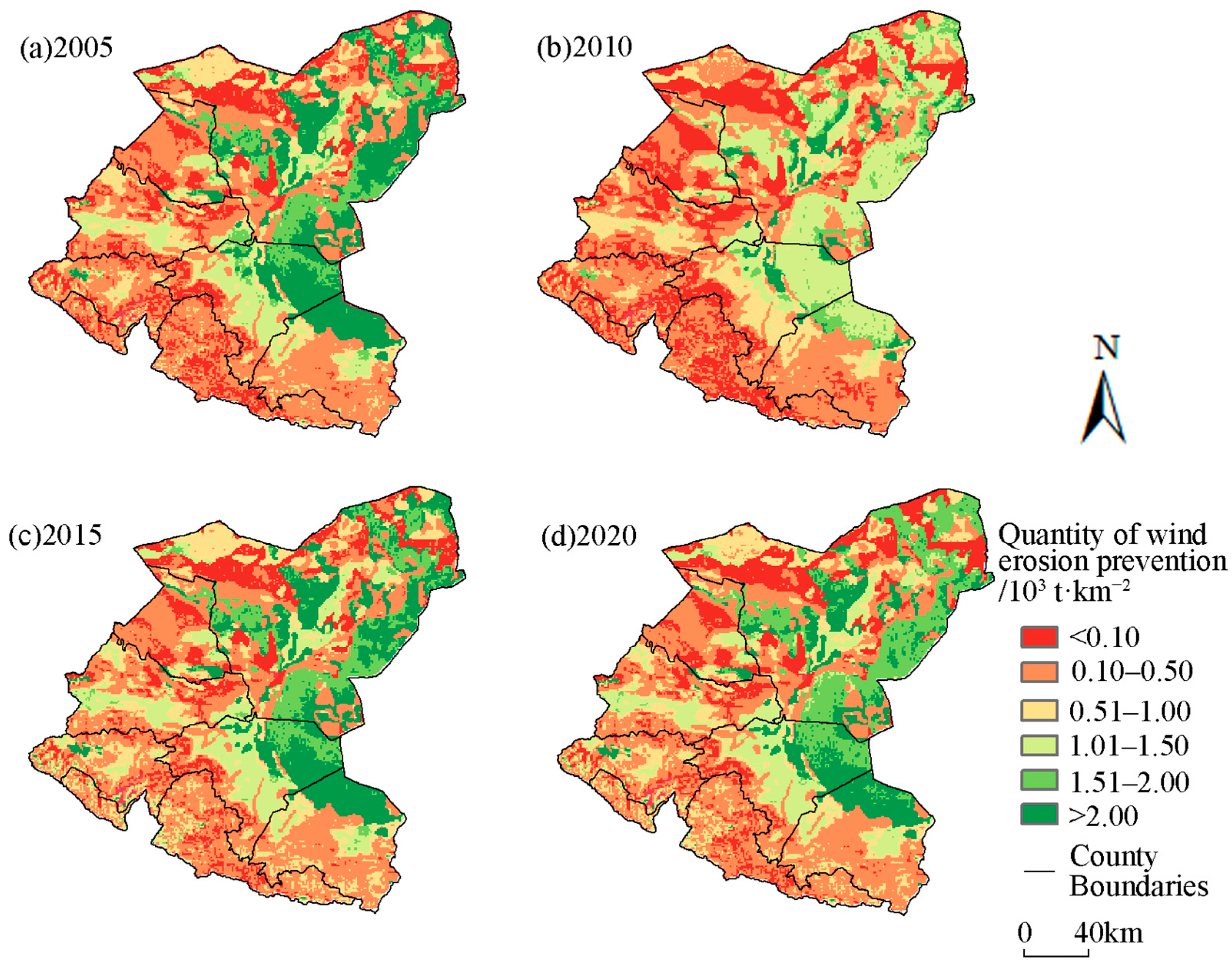
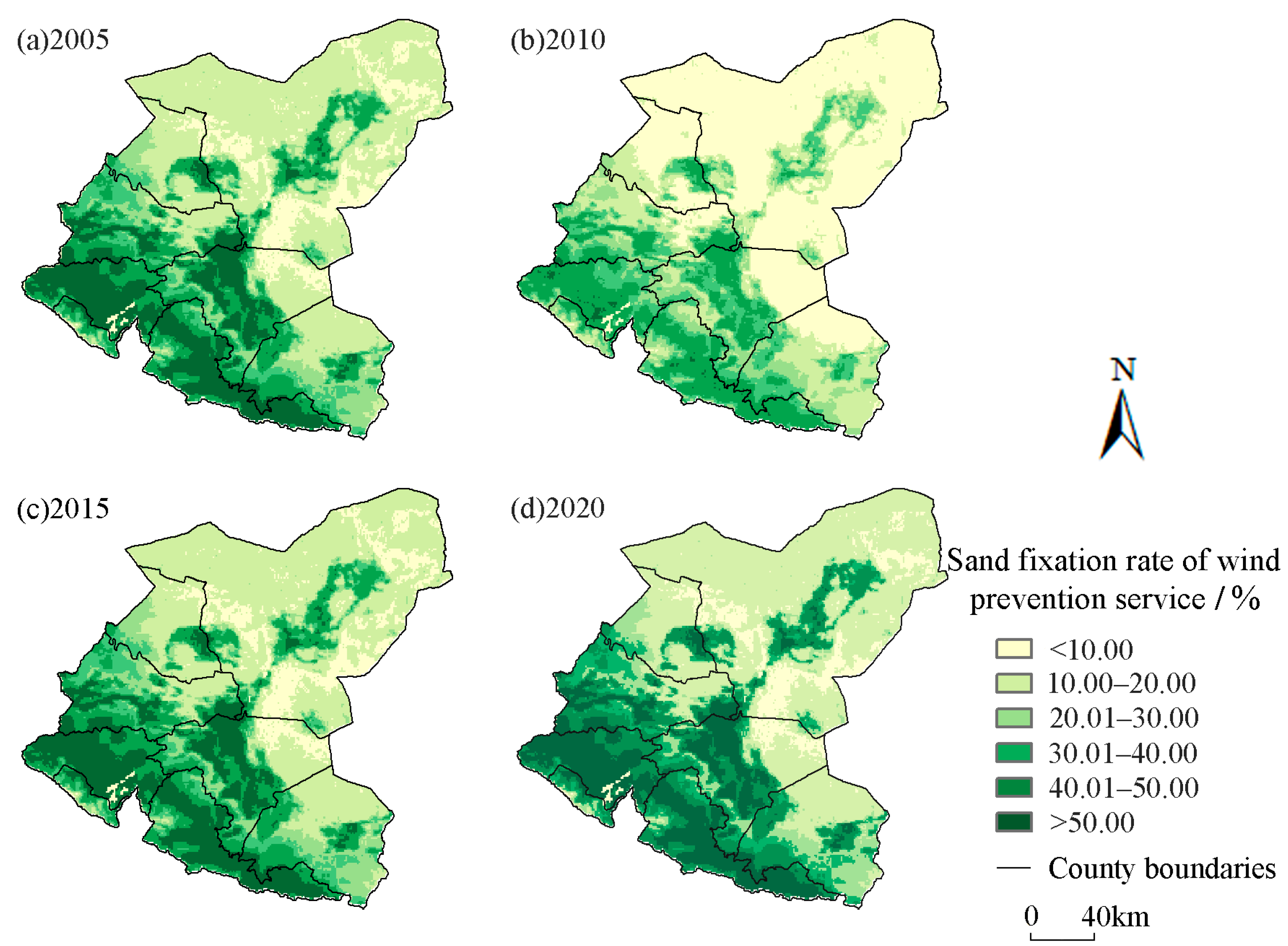
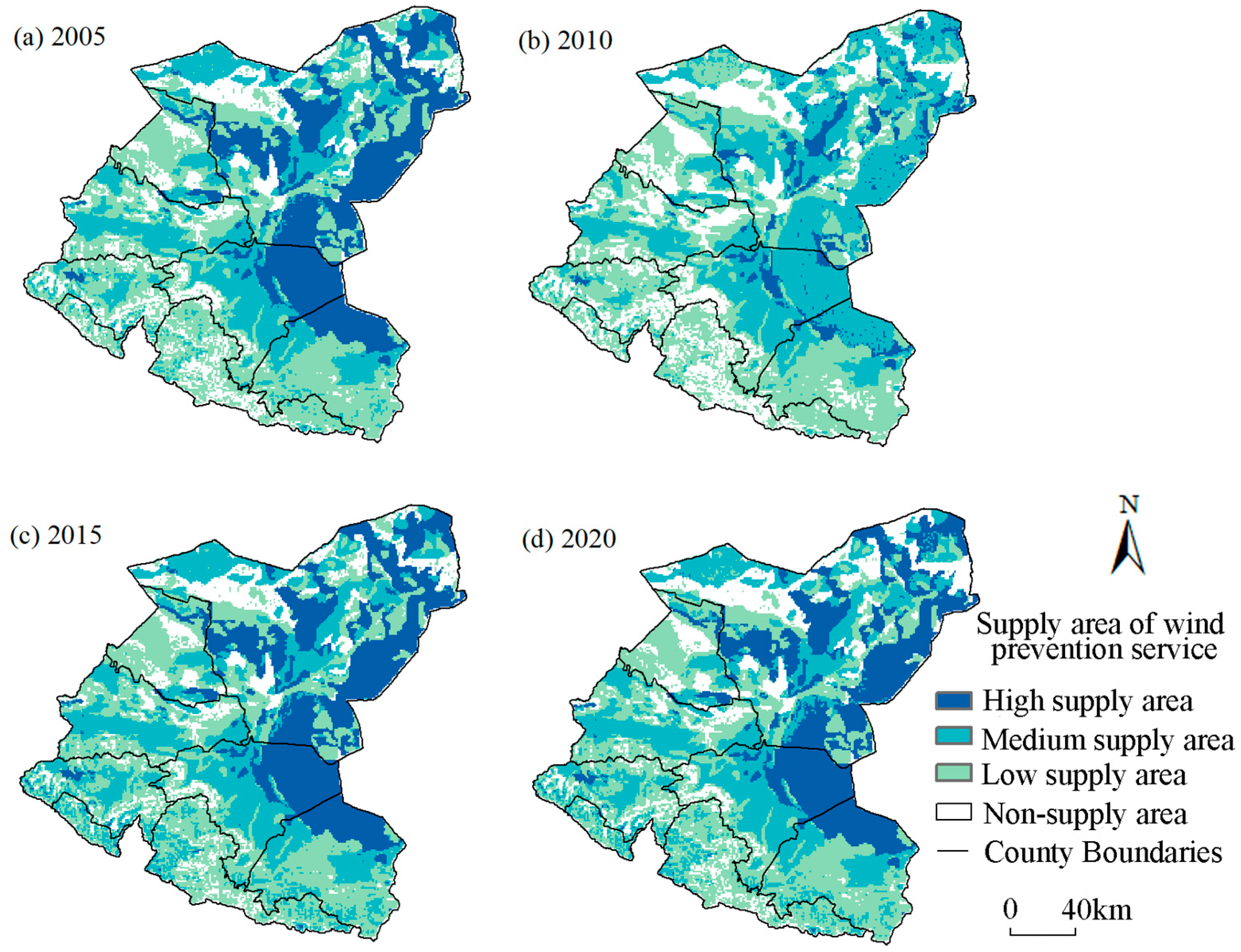
• From 2005 to 2020, the WEP services in SRB showed a differential distribution pattern from upstream to downstream, and a tendency of reducing, then increasing, then decreasing sand fixation overall was seen. The areas with higher sand fixation were mainly concentrated in the northeastern part and the junction zone between the oasis area and desert in the eastern part, and the amount of sand fixation in the north and south sides had a significant increase in the study period. In the watershed, Minqin County has the highest-density WEP services. The basic pattern of WEP rate in the same period is completely different from that of WEP services, showing a high south and low north trend, and meteorological factors have a great influence on the WEP capacity of SRB.
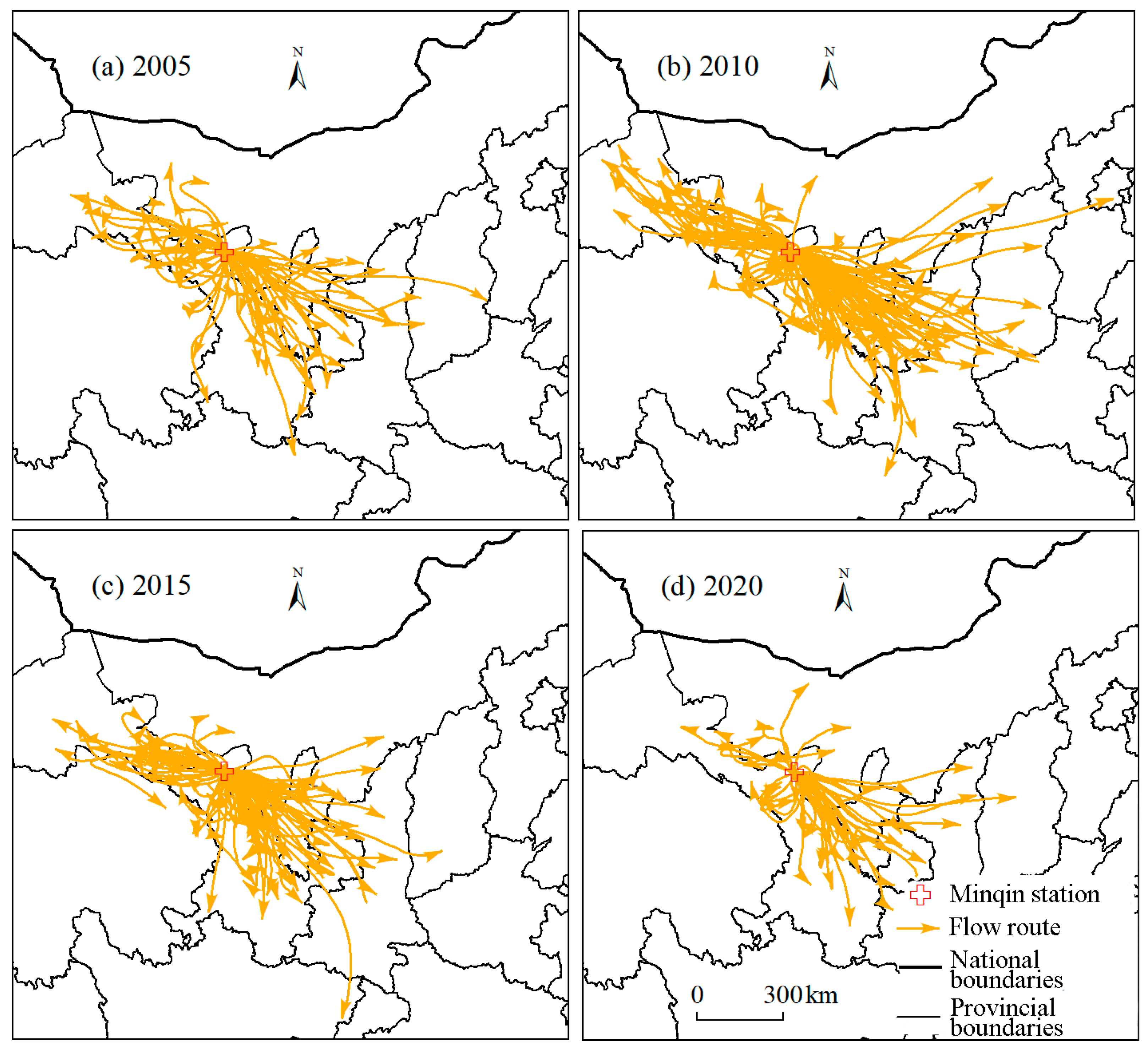
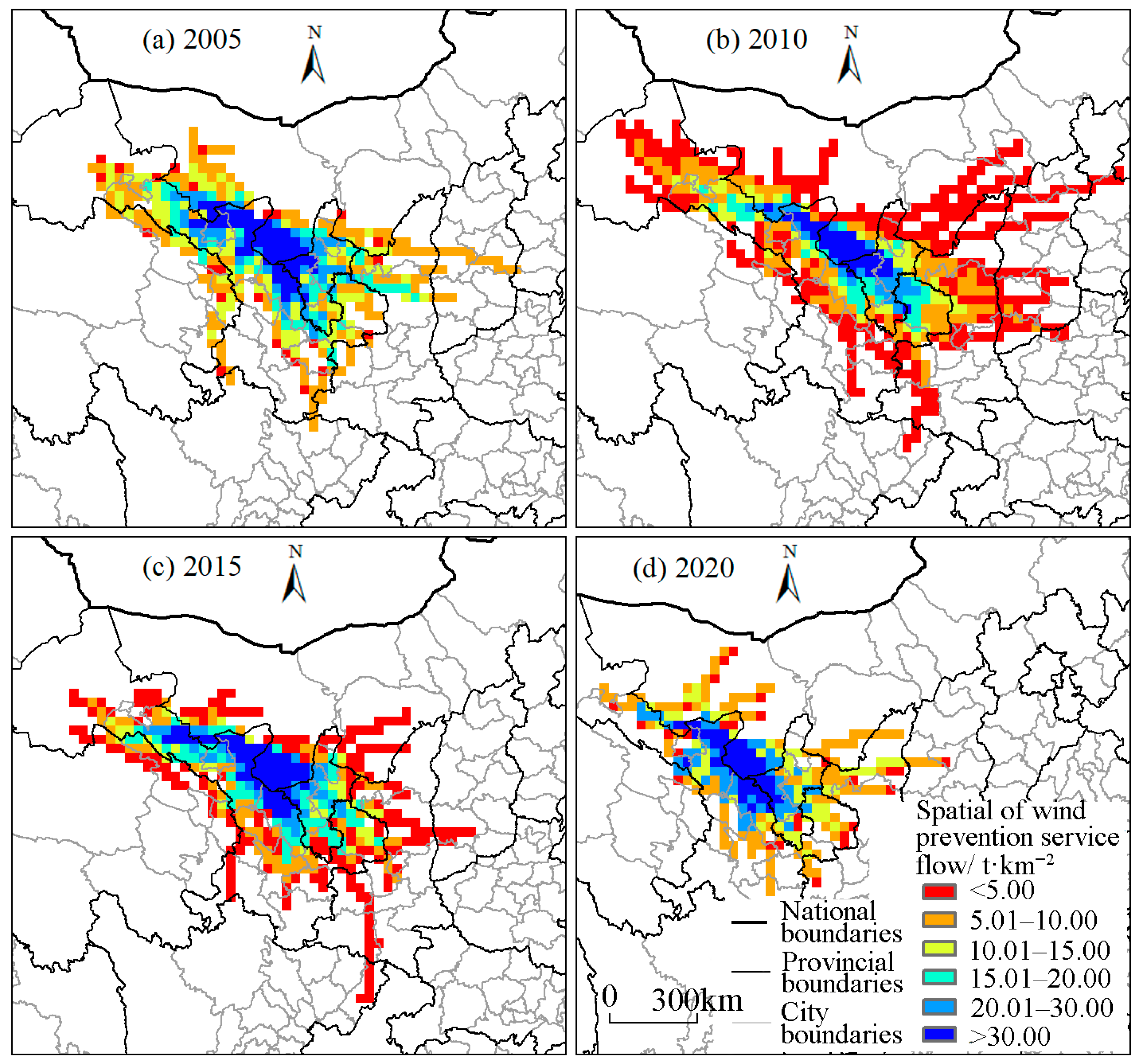
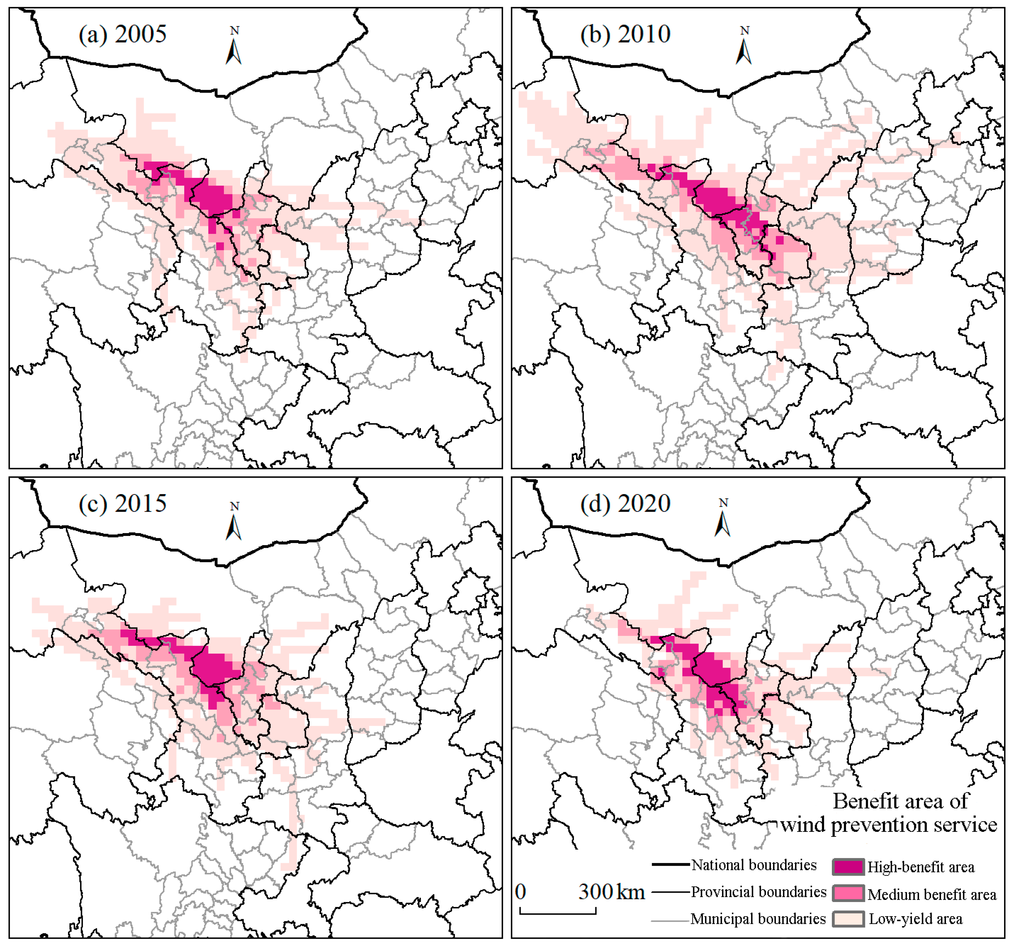
• The routes of WEP service flows in SRB show a northwest–southeast distribution pattern. In 2005, 2010, 2015, and 2020, the numbers of wind and sand service flow transmission routes recorded were 73, 134, 98, and 59, respectively, and the wind and sand records were mainly concentrated from March to May. WEP service flow has a very strong spatial extraterritorial effect, and the most important beneficiary regions of the WEP service flow in SRB are Gansu Province, Ningxia Hui Autonomous Region, and Inner Mongolia Autonomous Region. Among them, the routes were the most numerous and the flow range was the largest in 2010. The supply region of WEP and fixation services in the study area is contained within the beneficiary region, with significant cross-border beneficiary effects, and the largest beneficiary region in 2010, involving 47 cities in 9 provinces.

References

- Costanza, R.; Costanza, R.; de Groot, R.; Sutton, P.; van der Ploeg, S.; Anderson, S.J.; Kubiszewski, I.; Farber, S.; Turner, R.K. Changes in the global value of ecosystem services. Glob. Environ. Chang. 2014, 26, 152–158. [Google Scholar] [CrossRef]
- Parr, T.W.; Sier, A.R.; Battarbee, R.W.; Mackay, A.; Burgess, J. Detecting environmental change: Science and society-perspectives on long-term research and monitoring in the 21st century. Sci. Total Environ. 2003, 310, 1–8. [Google Scholar] [CrossRef]
- Jonathan, A.F.; Jonatnan, A.F.; Ruth, D.; Gregory, P.A.; Carol, B.; Gordon, B.; Stephen, R.C.; Stuart, C.F.; Michael, T.C.; Gretchen, C.D.; et al. Global Consequences of Land Use. Science 2005, 309, 570–574. [Google Scholar] [CrossRef]
- Wu, J. Landscape sustainability science: Ecosystem services and human well-being in changing landscapes. Landsc. Ecol. 2013, 28, 999–1023. [Google Scholar] [CrossRef]
- Bagstad, K.J.; Johnson, G.W.; Voigt, B.; Villa, F. Spatial dynamics of ecosystem service flows: A comprehensive approach to quantifying actual services. Ecosyst. Serv. 2013, 4, 117–125. [Google Scholar] [CrossRef]
- Serna-Chavez, H.M.; Schulp, C.J.E.; van Bodegom, P.M.; Bouten, W.; Verburg, P.H.; Davidson, M.D. A quantitative framework for assessing spatial flows of ecosystem services. Ecol. Indic. 2014, 39, 24–33. [Google Scholar] [CrossRef]
- Asensio, C.; Lozano, F.J.; Gallardo, P.A.; Giménez, A. Soil wind erosion in ecological olive trees in the Tabernas desert (southeastern Spain): A wind tunnel experiment. Solid Earth 2016, 7, 1233–1242. [Google Scholar] [CrossRef]
- Yang, W.Q.; Zhang, G.F.; Yang, H.M.; Lin, D.G.; Shi, P.J. Review and prospect of soil compound erosion. J. Arid. Land 2023, 15, 1007–1022. [Google Scholar] [CrossRef]
- Cham, D.D.; Son, N.T.; Minh, N.Q.; Thanh, N.T.; Dung, T.T. An Analysis of shoreline changes using combined multitemporal remote sensing and digital evaluation model. Civ. Eng. J. 2020, 6, 1–10. [Google Scholar] [CrossRef]
- Guo, B.; Zang, W.; Yang, X.; Huang, X.; Zhang, Y. Improved evaluation method of the soil wind erosion intensity based on the cloud-AHP model under the stress of global climate change. Sci. Total Environ. 2020, 746, 141271. [Google Scholar] [CrossRef]
- Ng, C.W.W.; Zhang, Q.; Zhou, C.; Ni, J.J. Eco-geotechnics for human sustainability. Sci. China (Technol. Sci.) 2022, 65, 2809–2845. [Google Scholar] [CrossRef]
- Zhang, M.; Viscarra Rossel, R.A.; Zhu, Q.; Leys, J.; Gray, J.M.; Yu, Q.; Yang, X. Dynamic Modelling of Water and Wind Erosion in Australia over the Past Two Decades. Remote Sens. 2022, 14, 5437. [Google Scholar] [CrossRef]
- May, J.; Hobbs, R.J.; Valentine, L.E. Are offsets effective? An evaluation of recent environmental offsets in Western Australia. Biol. Conserv. 2017, 206, 249–257. [Google Scholar] [CrossRef]
- Chepil, W.S. Relation of wind erosion to water- stable and dry clod structure of soil. Soil Sci. 1942, 55, 275–287. Available online: https://journals.lww.com/soilsci/fulltext/1943/04000/relation_of_wind_erosion_to_the_water_stable_and.1.aspx (accessed on 13 September 2023). [CrossRef]
- Chepil, W.S. Factors that influence clod structure and erodibility of soil by wind: III: Calcium carbonate and decomposed organic material. Soil Sci. 1954, 77, 473–480. Available online: https://journals.lww.com/soilsci/fulltext/1954/06000/factors_that_influence_clod_structure_and.8.aspx (accessed on 25 August 2023). [CrossRef]
- Zhao, W.; Hu, G.; Zhang, Z.; He, Z. Shielding effect of oasis-protection systems composed of various forms of wind break on sand fixation in an arid region: A case study in the hexi corridor, northwest China. Ecol. Eng. 2008, 33, 119–125. [Google Scholar] [CrossRef]
- Pierre, C.; Kergoat, L.; Bergametti, G.; Mougin, é.; Baron, C.; Abdourhamane Toure, A. Modeling vegetation and wind erosion from a millet field and from a rangeland: Two sahelian case studies. Aeolian Res. 2015, 19, 97–111. [Google Scholar] [CrossRef]
- Roels, B.; Donders, S.; Werger, M.J.A.; Dong, M. Relation of wind-induced sand displacement to plant biomass and plant sand-binding capacity. Acta Bot. Sin. 2001, 43, 979–982. [Google Scholar] [CrossRef]
- Wang, C.; Li, W.; Sun, M.; Wang, Y.T.; Wang, S.B. Exploring the formulation of ecological management policies by quantifying interregional primary ecosystem service flows in Yangtze River Delta region, China. J. Environ. Manag. 2021, 84, 112042. [Google Scholar] [CrossRef]
- Wang, L.J.; Zheng, H.; Chen, Y.Z.; Ouyang, Z.Y.; Hu, X.F. Systematic review of ecosystem services flow measurement: Main concepts, methods, applications and future directions. Ecosyst. Serv. 2022, 58, 101479. [Google Scholar] [CrossRef]
- Wang, Y.W.; Hong, S.; Wang, J.Z.; Lin, J.Y.; Mu, H.; Wei, L.Y.; Wang, Z.; Bryan, B.A. Complex regional telecoupling between people and nature revealed via quantification of trans-boundary ecosystem service flows. People Nat. 2022, 4, 274–292. [Google Scholar] [CrossRef]
- Fisher, B.; Turner, R.K. Ecosystem services: Classification for valuation. Biol. Conserv. 2008, 141, 1167–1169. [Google Scholar] [CrossRef]
- Fisher, B.; Turner, R.K.; Burgess, N.D.; Swetnam, R.D.; Balmford, A. Measuring, modeling and mapping ecosystem services in the eastern arc mountains of tanzania. Prog. Phys. Geogr. 2011, 35, 595–611. [Google Scholar] [CrossRef]
- Schröter, M.; Barton, N.D.; Remme, P.R.; Hein, L. Accounting for capacity and flow of ecosystem services: A conceptual model and a case study for Telemark, Norway. Ecol. Indic. 2014, 36, 539–551. [Google Scholar] [CrossRef]
- Schroeter, M.; Kraemer, R.; Remme, R.P.; van Oudenhoven, A.P.E. Distant regions underpin interregional flows of cultural ecosystem services provided by birds and mammals. Ambio 2020, 49, 1100–1113. [Google Scholar] [CrossRef] [PubMed]
- Yang, G.; Sun, R.; Jing, Y.; Xiong, M.; Li, J.; Chen, L. Global assessment of wind erosion based on a spatially distributed RWEQ model. Prog. Phys. Geogr. Earth Environ. 2022, 46, 28–42. [Google Scholar] [CrossRef]
- Fryrcar, D.W.; Chen, W.N.; Lester, C. Revised wind erosion equation. Ann. Arid. Zone 2001, 40, 265–279. [Google Scholar] [CrossRef]
- Zhang, W.B.; Xie, Y.; Liu, B.Y. Rainfall Erosivity estimation using daily rainfall amounts. Sci. Geogr. Sin. 2002, 22, 705–711. (In Chinese) [Google Scholar] [CrossRef]
- Jenness, J.S. Calculating landscape surface area from digital elevation models. Wildl. Soc. Bull. 2004, 32, 829–839. [Google Scholar] [CrossRef]
- Xu, J. A Study on the Spatial Flow of Ecosystem Services—Taking Ningxia Hui Autonomous Region as an Example. Ph.D. Thesis, University of Chinese Academy of Sciences, Beijing, China, 2019. (In Chinese). [Google Scholar]
- Guo, S.J.; Yang, Z.H.; Wang, Q.Q.; Wang, D.Z.; Wang, F.; Fan, B.L.; Zhang, Y.J.; Li, Y.J.; An, F.B. Sediment transport fluxes of wind-sand flows on different underlying surfaces of dry lake in the lower reaches of SRB. Sci. Silvae Sin. 2021, 57, 13–21. (In Chinese) [Google Scholar]
- Xie, G.D.; Liu, J.Y.; Xu, J.; Xiao, Y.; Zhen, L.; Zhang, C.S.; Wang, Y.Y.; Qin, K.Y.; Gan, S.; Jiang, Y. A spatio-temporal delineation of trans-boundary ecosystem service flows from Inner Mongolia. Environ. Res. Lett. 2019, 14, 065002. [Google Scholar] [CrossRef]
- Jooybari, S.A.; Peyrowan, H.; Rezaee, P.; Gholami, H. Evaluation of pollution indices, health hazards and source identification of heavy metal in dust particles and storm trajectory simulation using HYSPLIT model (Case study: Hendijan center dust, southwest of Iran). Environ. Monit. Assess. 2022, 194, 107. [Google Scholar] [CrossRef] [PubMed]
- Bera, B.; Bhattacharjee, S.; Sengupta, N.; Saha, S. Variation and dispersal of PM10 and PM2.5 during COVID-19 lockdown over Kolkata metropolitan city, India investigated through HYSPLIT model. Geosci. Front. 2022, 13, 291–302. [Google Scholar] [CrossRef]
- Trošić Lesar, T.; Filipčić, A. Lagrangian particle dispersion (HYSPLIT) model analysis of the sea breeze case with extreme mean daily PM10 concentration in Split, Croatia. Environ. Sci. Pollut. Res. 2022, 29, 73071–73084. [Google Scholar] [CrossRef] [PubMed]
- Roland, D.; Barbara, S.; Glenn, R. HYSPLIT Users Guide5.2; Air Resources Laboratory: College Park, MD, USA, 2022. Available online: https://www.ready.noaa.gov/hysplitusersguide (accessed on 19 September 2023).
- Wang, Y.Y.; Xiao, Y.; Xu, J.; Xie, G.D.; Qin, K.Y.; Liu, J.Y.; Niu, Y.N.; Gan, S.; Huang, M.D. Evaluation of Inner Mongolia Wind Erosion Prevention Service Based on Land Use and the RWEQ Model. J. Resour. Ecol. 2022, 13, 763–774. [Google Scholar] [CrossRef]
- Huang, M.D.; Xiao, Y.; Xu, J.; Liu, J.Y.; Wang, Y.Y.; Gan, S.; Lv, S.X.; Xie, G.D. A Review on the Supply-Demand Relationship and Spatial Flows of Ecosystem Services. J. Resour. Ecol. 2022, 13, 925–935. [Google Scholar] [CrossRef]
- Gong, G.L.; Liu, J.Y.; Shao, Q.Q. Wind erosion in Xilingol League, Inner Mongolia since the 1990s using the Revised Wind Erosion Equation. Prog. Geogr. 2014, 33, 825–834. (In Chinese) [Google Scholar] [CrossRef]
- Liu, C.F.; Wang, J.X.; Xu, X.Y. Regional division and standard accounting of ecological compensation from the perspective of ecosystem service flow: A case study of SRB. China Popul. Resour. Environ. 2021, 31, 157–165. (In Chinese) [Google Scholar] [CrossRef]
- Liu, J.; Guo, Z.L.; Chang, C.P.; Wang, R.D.; Li, J.F.; Li, Q.; Wang, X.Y. Potential wind erosion simulation in the agro-pastoral ecotone of northern China using RWEQ and WEPS models. J. Desert Res. 2021, 41, 27–37. (In Chinese) [Google Scholar]
- Li, J. Shaanxi Will Be Hit again by Strong Winds, Cool Temperatures, and Sandstorms Starting from the 25th. Chinanews, 24 April 2010. Available online: http://www.chinanews.com.cn/gn/news/2010/04-24/2245356.shtml (accessed on 19 September 2023). (In Chinese).
- Fang, L.Q. Analysis of the April 2010 atmospheric circulation and weather. Meteorol. Phenom. 2010, 36, 174–179. (In Chinese) [Google Scholar]
Disclaimer/Publisher’s Note: The statements, opinions and data contained in all publications are solely those of the individual author(s) and contributor(s) and not of MDPI and/or the editor(s). MDPI and/or the editor(s) disclaim responsibility for any injury to people or property resulting from any ideas, methods, instructions or products referred to in the content. |
© 2023 by the authors. Licensee MDPI, Basel, Switzerland. This article is an open access article distributed under the terms and conditions of the Creative Commons Attribution (CC BY) license (https://creativecommons.org/licenses/by/4.0/).
Share and Cite
Pan, J.; Wei, J.; Xu, B. Simulation of the Spatial Flow of Wind Erosion Prevention Services in Arid Inland River Basins: A Case Study of Shiyang River Basin, NW China. Atmosphere 2023, 14, 1781. https://doi.org/10.3390/atmos14121781
Pan J, Wei J, Xu B. Simulation of the Spatial Flow of Wind Erosion Prevention Services in Arid Inland River Basins: A Case Study of Shiyang River Basin, NW China. Atmosphere. 2023; 14(12):1781. https://doi.org/10.3390/atmos14121781
Chicago/Turabian StylePan, Jinghu, Juan Wei, and Baicui Xu. 2023. "Simulation of the Spatial Flow of Wind Erosion Prevention Services in Arid Inland River Basins: A Case Study of Shiyang River Basin, NW China" Atmosphere 14, no. 12: 1781. https://doi.org/10.3390/atmos14121781
APA StylePan, J., Wei, J., & Xu, B. (2023). Simulation of the Spatial Flow of Wind Erosion Prevention Services in Arid Inland River Basins: A Case Study of Shiyang River Basin, NW China. Atmosphere, 14(12), 1781. https://doi.org/10.3390/atmos14121781