Article

Spatial Distribution and Inter-City Transport of PM2.5 Concentrations from Vehicles in the Guanzhong Plain in Winter

1
School of Water and Environment, Chang’an University, Xi’an 710064, China
2
School of Energy and Architecture, Xi’an Aeronautical Institute, Xi’an 710077, China
3
School of Architectural Engineering, Chang’an University, Xi’an 710064, China
4
Key Laboratory of Subsurface Hydrology and Ecological Effect in Arid Region of Ministry of Education, Chang’an University, Xi’an 710064, China
*
Author to whom correspondence should be addressed.
Atmosphere 2023, 14(12), 1748; https://doi.org/10.3390/atmos14121748
Submission received: 27 October 2023 / Revised: 21 November 2023 / Accepted: 26 November 2023 / Published: 28 November 2023
(This article belongs to the Section Air Quality)

Abstract

:
Regional atmospheric environmental problems have become increasingly prominent due to continuous urbanization in China. In this study, the Weather Research and Forecasting (WRF) model coupled with the California Puff (CALPUFF) air quality model was applied to analyze the spatial distribution and inter-city transport of primary and secondary PM2.5 concentrations from vehicles in the Guanzhong Plain (GZP) in January 2019. The results show that the secondary PM2.5 concentration emitted by vehicles was more easily dispersed than primary PM2.5. The maximum hourly average concentrations of primary PM2.5, secondary inorganic aerosol (SIA), and secondary organic aerosol (SOA) were about 18, 9, and 2 µg/m3, respectively. Exhaust emission and secondary NO3 were the main contributors to the total PM2.5 concentration from vehicles, accounting for about 52% and 32%, respectively. The maximum contribution of vehicle emissions to the ambient PM2.5 concentration was about 19%. Inter-city transport contributed about 33% of the total PM2.5 concentration from vehicles in cities in the GZP on average. Among the PM2.5 components transported in each city, SIA was the most abundant, followed by primary PM2.5, and SOA was the least. These findings will provide valuable insights for mitigating the regional PM2.5 pollution caused by near-surface sources in urban agglomerations.

1. Introduction

In recent years, the rapid development of the economy and the acceleration of industrialization and urbanization have led to an increasingly serious air pollution problem in China [1,2]. Regional air pollution caused by fine particulate matter (PM2.5) frequently occurs in several key regions in China, such as the Beijing-Tianjin-Hebei (BTH) region [3,4], the Yangtze River Delta (YRD) [5,6], and the Guanzhong Plain (GZP) [7,8,9]. High ambient PM2.5 concentrations have negative impacts on atmospheric visibility, regional climate, and human health. Long-term exposure to ambient PM2.5 has caused approximately 4.2 million premature fatalities annually from 2019 onwards according to the World Health Organization (WHO) [10]. Owing to the severe detrimental effects of PM2.5, the Chinese government has successively enacted a number of rigorous air pollution control measures in recent years to improve air quality [11,12,13]. Currently, although China has substantially reduced its PM2.5 pollution, the annual average PM2.5 concentration in some highly polluted cities or regions still exceeds the limit of 35 µg/m3 set by the China Class II Environmental Air Quality Standard and the limit of 10 µg/m3 set by the WHO. According to statistics [14], the total number of vehicles in China reached 395 million in 2021, and the emission of particulate matter reached 69,000 tons. With the continuous and rapid increase in vehicle population in recent years, vehicle emissions have become a primary contributor to ambient PM2.5 [15,16,17]. The total PM2.5 emitted by vehicles comes not only from direct exhaust emissions, but also from brake wear, tire wear, road wear, and re-suspended road dust, as well as secondary inorganic aerosol (SIA) and secondary organic aerosol (SOA) generated by the chemical conversion of gaseous precursors from exhaust [18]. In addition, vehicle emissions belong to near-surface sources, close to human activity areas, and pose a greater threat to human health than other anthropogenic sources. As a consequence, reducing the impact of vehicle emissions on ambient PM2.5 has emerged as a challenging issue of concern.
Given that air quality monitoring can solely offer the concentration data at sensor-equipped points, many scholars estimate the entire spatial distribution of the PM2.5 concentration from vehicles by using air quality models. Previous studies mainly focused on simulating the dispersion of primary PM2.5 emitted only by vehicle exhaust on a single road [19,20], multiple roads [21,22], or all urban roads [23,24,25]. Additionally, these studies have investigated the effects of variables such as traffic conditions [26,27], surrounding buildings [19], topography [28], and meteorology [26,29] on the spatial distribution of the PM2.5 concentration. However, there are few studies on the dispersion of the non-exhaust PM2.5 and the exhaust secondary PM2.5 (generated by the gas-particle transformation of gaseous precursors from vehicle tailpipes). The dispersion mechanism of non-exhaust PM2.5 and exhaust secondary PM2.5 in the atmosphere differs significantly from that of primary PM2.5 from exhaust. First, the dispersion of primary PM2.5 from exhaust and non-exhaust emissions varies in the physical parameters, including emission height, emission temperature, and flow disturbance mode. Second, complex chemical reactions accompany the dispersion process of SIA and SOA, which are impacted in real time by various environmental factors such as solar radiation, relative humidity, temperature, background ozone concentration, etc., [30,31]. Several studies have provided evidence that the non-exhaust emissions of PM2.5 are as much and often more than exhaust emissions in cities [21,32]. Additionally, the presence of secondary PM2.5 concentration is a crucial component of the total PM2.5 concentration emitted by vehicles [28]. Hence, it is crucial to carry out simulation research on the dispersion of PM2.5 produced by all emission routes of vehicles in the atmosphere, which is of great significance to determine the real contribution of vehicle emissions to ambient PM2.5 levels.
Meanwhile, numerous researchers have reported that PM2.5 pollution in a city is related to both local emissions and transport from surrounding cities [33,34]. Especially in economically developed and densely populated urban agglomerations, PM2.5 pollution is no longer confined to single cities, and the variability of PM2.5 pollution between cities shows clear synchronization. Although local emissions of PM2.5 are a significant factor in local pollution, the cross-boundary transmission of pollutants between cities also has an inevitable impact on regional pollution. Therefore, the government has proposed “inter-regional prevention and control” to further control ambient PM2.5 pollution [35]. Previous studies have mostly focused on the transport of PM2.5 from elevated sources between cities or regions [36,37], while studies exploring the inter-city transport of secondary PM2.5 focused on that emitted by vehicles near the ground.
To fill the gaps mentioned above, this study selected the GZP as the research area. Since the ambient air quality in January of the winter is the worst in this region every year, and the annual average PM2.5 concentration in 2019 is the highest in recent years, January 2019 was taken as the research period. Considering both the exhaust and non-exhaust emissions of vehicles, this study estimated the emission inventory of SO2, NOx, VOCs, and primary PM2.5 from vehicles by using the emission factor method. Then, the Weather Research and Forecasting (WRF) model and the California Puff (CALPUFF) air quality model were utilized to simulate the dispersion and inter-city transport of PM2.5 emitted by vehicles in cities in the GZP in winter. Subsequently, the contribution of the total PM2.5 concentration from vehicle emissions to the ambient PM2.5 concentration was also analyzed. The results of this study provide some scientific references for the control of PM2.5 pollution from vehicles in the GZP.

2. Materials and Methods

2.1. Study Area

The Guanzhong Plain, located in the central region of Shaanxi Province, encompasses five prefecture-level cities: Xi’an (XA), Xianyang (XY), Weinan (WN), Baoji (BJ), and Tongchuan (TC) (Figure 1). It is surrounded by mountains on three sides, bordered by the Qinghai-Tibet Plateau to the west, the Qinling Mountains to the south, and the Loess Plateau to the north, forming a horn-shaped opening in the east–west direction. The GZP is the fourth largest plain in China, with a length of approximately 380 km from east to west and a width of approximately 260 km from north to south, and a total area of about 55,465 km2. Its topography is high in the west and low in the east, with an average elevation of 500 m. The GZP is the starting point and gateway of China’s Belt and Road initiative, as well as the political, economic, cultural, and educational center of Shaanxi Province, with a residential population of about 24.99 million by 2021 [38].

2.2. Method for Calculating Vehicle Emissions

The accurate and comprehensive vehicle emission inventory serves as the fundamental basis for simulating the effective dispersion and transport of vehicle pollutants. In this study, we employed the emission factor method to estimate vehicle emissions in the GZP. The emissions of pollutants can be calculated based on the emission factors, the vehicle population, and the annual average number of vehicle kilometers traveled (VKT). The calculation formula is presented as follows:
EQ k = i j EF i ,   j   ×   P i ,   j   ×   VKT i ,   j   ×   10 - 6
where EQ is the annual emissions of conventional pollutants (tons); EF is the vehicle emission factor (g/km); P is the vehicle population; VKT is the annual average number of vehicle kilometers traveled (in km/vehicle); k is the pollutant type, including SO2, NOx, VOCs, and primary PM2.5 in this study; i is the vehicle type, including eight vehicle types (light-duty passenger vehicle, medium-duty passenger vehicle, heavy-duty passenger vehicle, light-duty truck, medium-duty truck, heavy-duty truck, motorcycle, and low-speed vehicle (including three-wheeled vehicles and low-speed trucks)); j is the vehicle emission standard, including six categories from China I to China VI.
The EF was determined using the Motor Vehicle Emission Simulator (MOVES) model, a new-generation regulatory emission model developed by the United States Environmental Protection Agency (USEPA). The model has gained widespread adoption in the establishment of a vehicle emission inventory both domestically and abroad because of its high calculation accuracy and rich pollutant types [26,39,40,41]. Due to the fact that the MOVES model is constructed based on a large amount of on-board and bench test data from the United States, in order to ensure that the model can accurately reflect vehicle emission information in the GZP, we localized the input parameters in the MOVES model, which mainly include vehicle age distribution, road type distribution, vehicle speed distribution, fuel information, and meteorological information, etc. The age distribution of various types of vehicles was obtained by consulting the statistical yearbooks of five cities and conducting an on-site sampling survey at the vehicle administration. Through the field survey of various roads in the GZP, all roads in this region were classified and matched with the road types in the model. In this study, 50 typical vehicles were installed with GPS equipment and continuously monitored for one month, so as to obtain the speed distribution information of various types of vehicles. The fuel parameter information in the model was modified by referring to the composition standards of China’s automotive gasoline, diesel, and natural gas. Meteorological information was obtained from meteorological stations in each city. The P was derived from the statistical yearbooks published by various cities in the GZP. In 2019, the total vehicle population in the GZP was 5.30 million, of which XA, WN, XY, BJ, and TC accounted for 65.4%, 13.6%, 9.6%, and 2.4%, respectively. In addition, the population of gasoline vehicles, diesel vehicles, natural gas vehicles, and new energy vehicles in this region was 4.82 million, 329,800, 66,900, and 82,600, respectively. The VKT was obtained through an actual survey of local vehicles or from the annual report prepared by local vehicle inspection agencies.

2.3. Method for Calculating the Dispersion and Inter-City Transport of PM2.5

Air quality models are practical and cost-effective tools for quantifying the dispersion, transport, transformation, and removal processes of emitted air pollutants in the atmosphere [42,43]. Currently, air quality models such as AERMOD, CALPUFF, CMAQ, and CAMx have been widely used to investigate air pollution issues in various regions across the globe [44,45,46,47]. Compared with other air quality models, the CALPUFF model exhibits several advantages, including its wide applicability, high simulation accuracy, and fast operation speed, particularly in complex terrain conditions. Hence, it has been recommended by the USEPA as a preferred model and has gained widespread utilization in numerous countries. In addition, many scholars have successfully simulated the dispersion of pollutants emitted by vehicles using the CALPUFF model [20,26,28,29]. Therefore, the CALPUFF model was selected in this study to estimate the spatial distribution and inter-city transport of PM2.5 concentrations from vehicles in the GZP. Additionally, the WRF model was engaged to provide an initial driving meteorological field for pollutant dispersion for the CALPUFF model.
The WRF model is a mesoscale numerical weather prediction system that can meet the requirements of meteorological research and operational forecasting across scales ranging from a few kilometers to thousands of kilometers. In this study, the WRF model (version 3.9.1) was configured with two nested domains (see Figure 1), and the output data of the inner domain were used to generate the large-scale initial guess meteorological fields for the CALPUFF model system. The outer domain (D1) was of a 1224 km×1008 km extent in the horizontal region, with a resolution of 9 km, covering most of the middle part of China. The inner domain (D2) was of a 714 km×546 km extent in the horizontal region, with a resolution of 3 km, encompassing nearly the entirety of Shaanxi Province. Both D1 and D2 were centered on the location of the Bell Tower (108.95° E, 34.26° N) in Xi’an, and both have 32 vertical layers up to 50 hPa. The initial and boundary conditions for the WRF model were obtained from the Global Forecast System Final Analysis (FNL) of the National Center for Environmental Prediction (NCEP), which were acquired at 6 h intervals with a horizontal resolution of 1° (approximately 111 km). The parameterization schemes employed in the WRF model are presented in Table 1.
The CALPUFF model is a multi-layer, multi-species, non-steady-state Gaussian puff dispersion model that can simulate the atmospheric dispersion process of continuous or time-varying pollutant releases from point, line, area, or volume sources [31,48,49,50]. When calculating plume dispersion using Gaussian equations, the model incorporates considerations of plume rise, plume buoyancy, vertical wind shear, and building downwash. The CALPUFF model is commonly used to study the long-range dispersion and transport of multiple air pollutants by considering the effects of temporally and spatially varying meteorological conditions, especially for distances above 50 km [44,51]. The CALPUFF model system is mainly composed of four parts: a geographic data preprocessor, a diagnostic three-dimensional meteorological model (CALMET), an air quality dispersion model (CALPUFF), and a postprocessor (CALPOST). The terrain and land-use data required by the preprocessor in this study were derived from the United States Geological Survey (USGS) data. The CALMET module is utilized to diagnose and correct the initial guessed meteorological field generated by the WRF model, thereby obtaining a more accurate final meteorological field. The CALPUFF model is the core module of the whole air quality dispersion system, which uses the final meteorological field generated by CALMET to simulate the dispersion, transport, transformation, and deposition of pollutants discharged by pollution sources. The CALPOST model post-processes the results from the CALPUFF model and finally generates the concentrations of pollutants in specified gridded cells.
In this study, the CALPUFF model (version 7.3.2) was configured with a domain with a grid number of 250 × 150 and a horizontal resolution of 2 km, which was smaller than the D2 of the WRF model, but completely covered the whole GZP (see Figure 1). Ten height layers were set in the vertical dimension, each height layer was 0, 20, 50, 100, 200, 300, 500, 1000, 2000, and 3000 m from the ground level. The main parameter settings for CALPUFF are given in Table 2. The RIVAD+ISORROPIA+CalTechSOA chemical transformation scheme was used to simultaneously simulate the conversion of gaseous precursors emitted by vehicles to secondary inorganic aerosols and secondary organic aerosols. In this scheme, the RIVAD+ISORROPIA part was used for the conversion of SO2 and NOx to secondary sulfates (SO42−) and nitrates (NO3), while the CalTechSOA part was used for the conversion of VOCs to SOA. Since the chemical conversion in CalTechSOA only involves four VOCs (toluene, xylene, long-chain alkane, and polycyclic aromatic hydrocarbons), this study allocated the total VOCs emissions from vehicles to the above four components according to the research results of Tan et al. and Huang et al. [52,53]. For the background ozone and ammonia concentrations involved in the above reactions, we obtained them respectively from the state-controlled air quality monitoring stations in GZP and the research results of Wu et al. [54]. In addition, dry and wet deposition was also considered in the simulation of this study.

3. Results and Discussion

3.1. Emission Inventory of Vehicle Pollutants

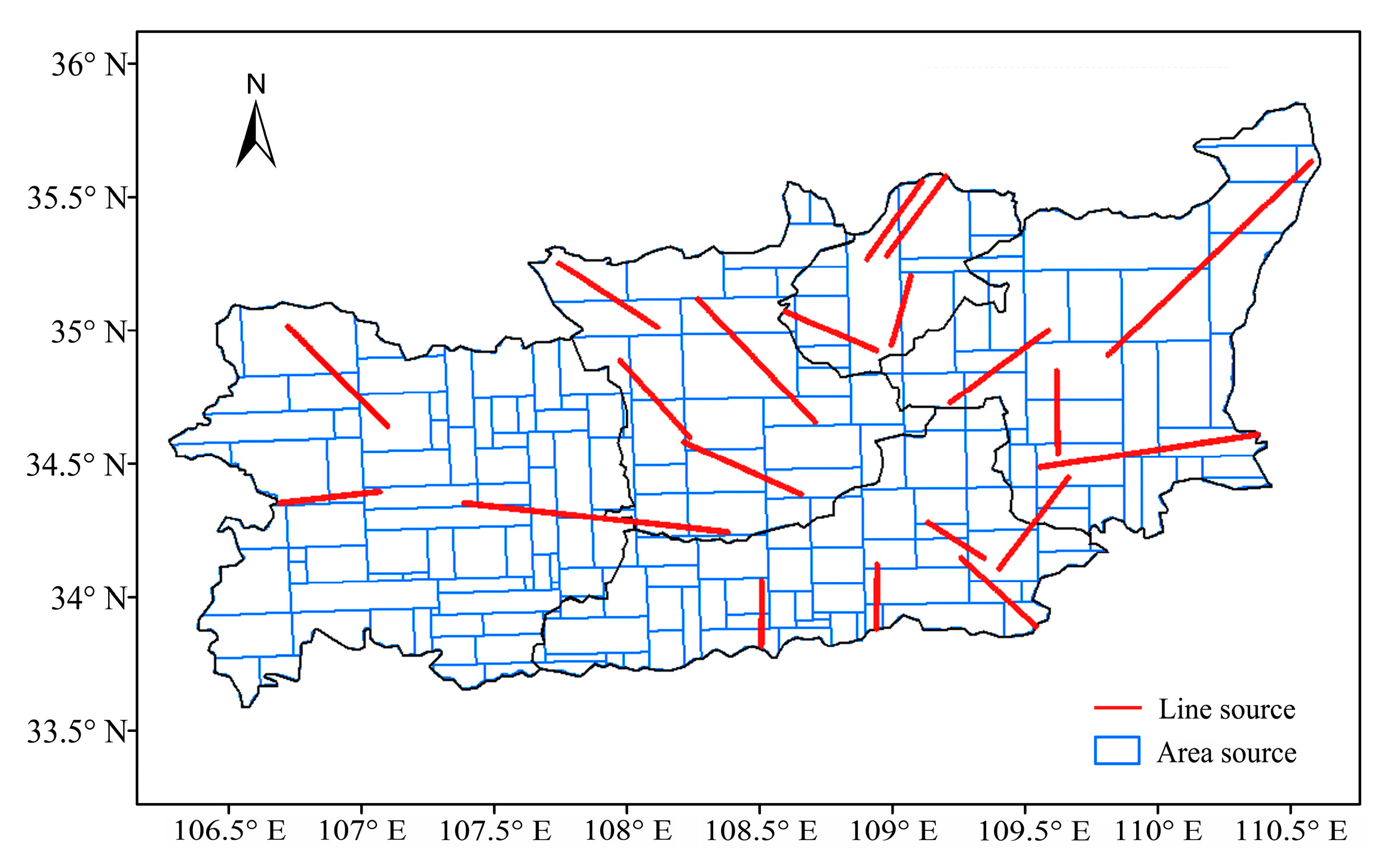
Based on the localized modified MOVES model and field survey data, the emissions of SO2, NOx, VOCs, and primary PM2.5 from vehicles in various cities in the GZP were calculated using Equation (1), as shown in Table 3. In January 2019, the vehicle emissions of SO2, NOx, VOCs, and primary PM2.5 in the GZP were 17.92, 6282.82, 2414.38, and 345.35 t, respectively. Among all cities, XA exhibited the highest emissions of the above four pollutants, accounting for 55.97%, 52.41%, 46.04%, and 46.77% of their total emissions, respectively, followed by WN, and TC had the smallest emissions. This is mainly related to the differences in vehicle population and road network density among cities. In the gaseous precursors of SIA from vehicles in the GZP, the emission of NOx was two orders of magnitude higher than that of SO2. For the emission pathways of primary PM2.5 from vehicles, this study considered exhaust, brake wear, and tire wear, which accounted for 83.5%, 13.77%, and 2.73% of primary PM2.5 emissions from vehicles in the GZP, respectively. When the emissions of vehicle pollutants were input into the CALPUFF model as emission sources, the maximum number of line sources and area sources that can be input into the model are 24 and 200, respectively. On account of the dense and complex road network in the GZP, 20 line sources and 136 area sources were obtained by equivalent configuration according to the spatial distribution of pollutant emissions from vehicles in this region. The allocation results of line sources and area sources are shown in Figure 2.

3.2. Evaluation of Meteorological Simulations

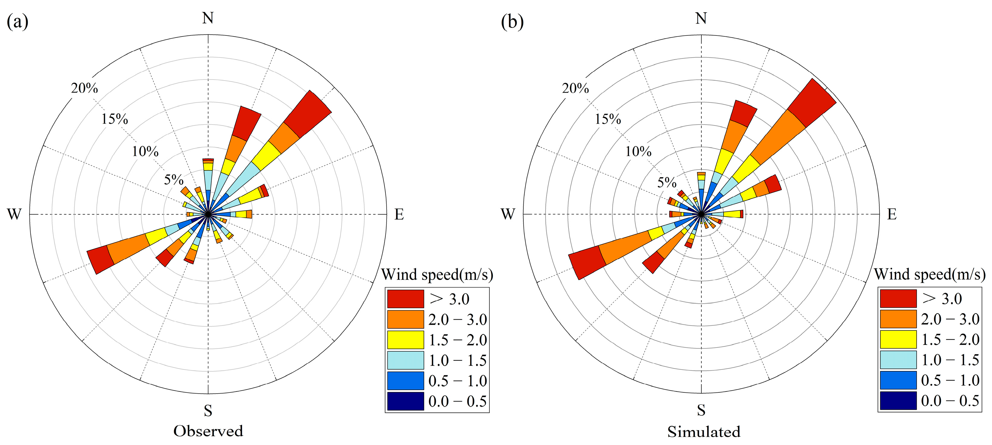
To assess the reliability of the meteorological simulation results, a comparison was made between the modeled data and the observed data from five typical meteorological sites in the GZP. These sites are situated in five distinct cities (see Figure 1), with an observation height of 2 m for temperature (T) and relative humidity (RH), and 10 m for wind direction (WD) and speed (WS). The simulation results were obtained by extracting the meteorological parameters at the same position and height as the above five sites in the simulated meteorological field. Figure 3 shows the simulated and observed wind rose plots in January 2019 in the GZP. Influenced by the local topography and monsoon, the prevailing wind directions were northeast and southwest. The occurrence frequency of the prevailing wind directions and the occurrence frequency of the high wind speed in the prevailing wind directions were slightly higher in the simulated results than in the observed results, which indicated that the WRF/CALMET model had an enhancement effect on the prevailing winds. But in general, the simulated results of wind direction and wind speed agreed well with the observed data.
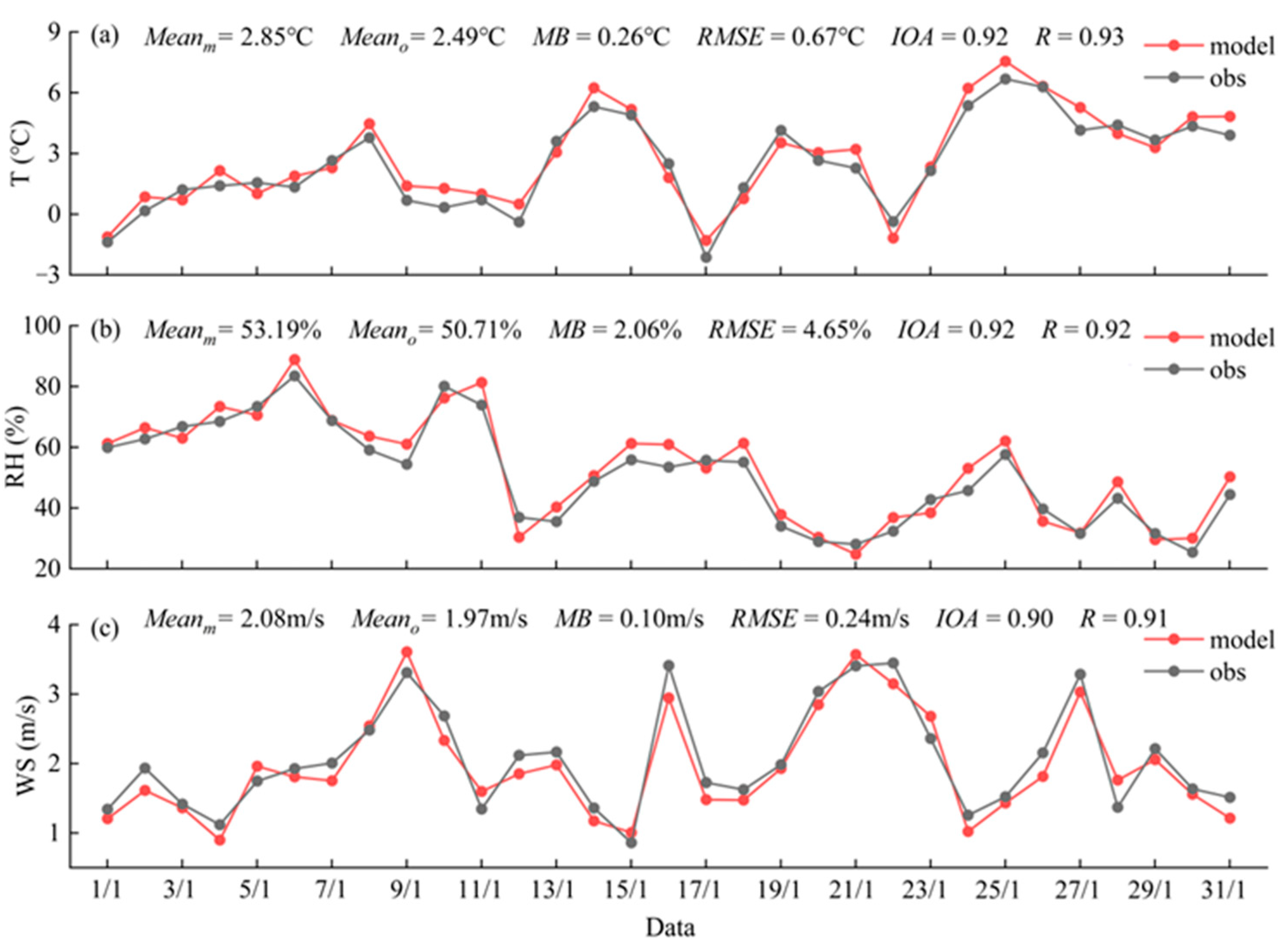
The daily variation in the average values of T, RH, and WS obtained from simulation and observation at all sites in January 2019 is presented in Figure 4. Additionally, four statistical indicators, including the mean bias (MB), the root mean square error (RMSE), the index of agreement (IOA), and the Pearson correlation coefficient (R), were employed to evaluate the performance of the WRF/CALMET model by comparing the simulated results with the observed values. In Figure 4, the daily variation curves of the simulated values of T, RH, and WS were slightly higher than those of the observed values. The simulated mean values of T, RH, and WS were 2.85 °C, 53.19%, and 2.08 m/s, respectively, while the observed mean values were 2.49 °C, 50.71%, and 1.97 m/s, respectively. The above results indicated that T, RH, and WS were overestimated in the simulation. In statistical indicators, MB and RMSE reflect the systematic error and the square root of the mean squared error, respectively. The closer their values are to 0, the more accurately the simulated values match with the observed data [30,55]. In the simulation results of this study, the MB and the RMSE values were as low as 0.26 and 0.67 °C for T, 2.06 and 4.65% for RH, and 0.1 and 0.24 m/s for WS, respectively. The IOA value always ranges from 0 to 1, where 0 represents the theoretical minimum value for an inaccurate prediction, and 1 represents a perfect agreement between the predicted and actual values. Normally, when the IOA is above 0.5, the simulation results are considered to be credible to some degree [30,56]. In this study, the IOA values for T, RH, and WS were all close to 1, with values of 0.92, 0.92, and 0.90, respectively. The value of R varies from −1.0 to 1.0, with −1 representing a perfect negative correlation between the simulated and observed values, and 1 representing a perfect positive correlation [55]. The R values were 0.93 for T, 0.92 for RH, and 0.91 for WS, indicating a high level of correlation and agreement between the calculated results and the observations. Overall, these statistical indicators indicated that the meteorological simulation results of the WRF/CALMET model in this study had sufficient reliability and precision.

3.3. Spatial Distribution of PM2.5 Concentrations

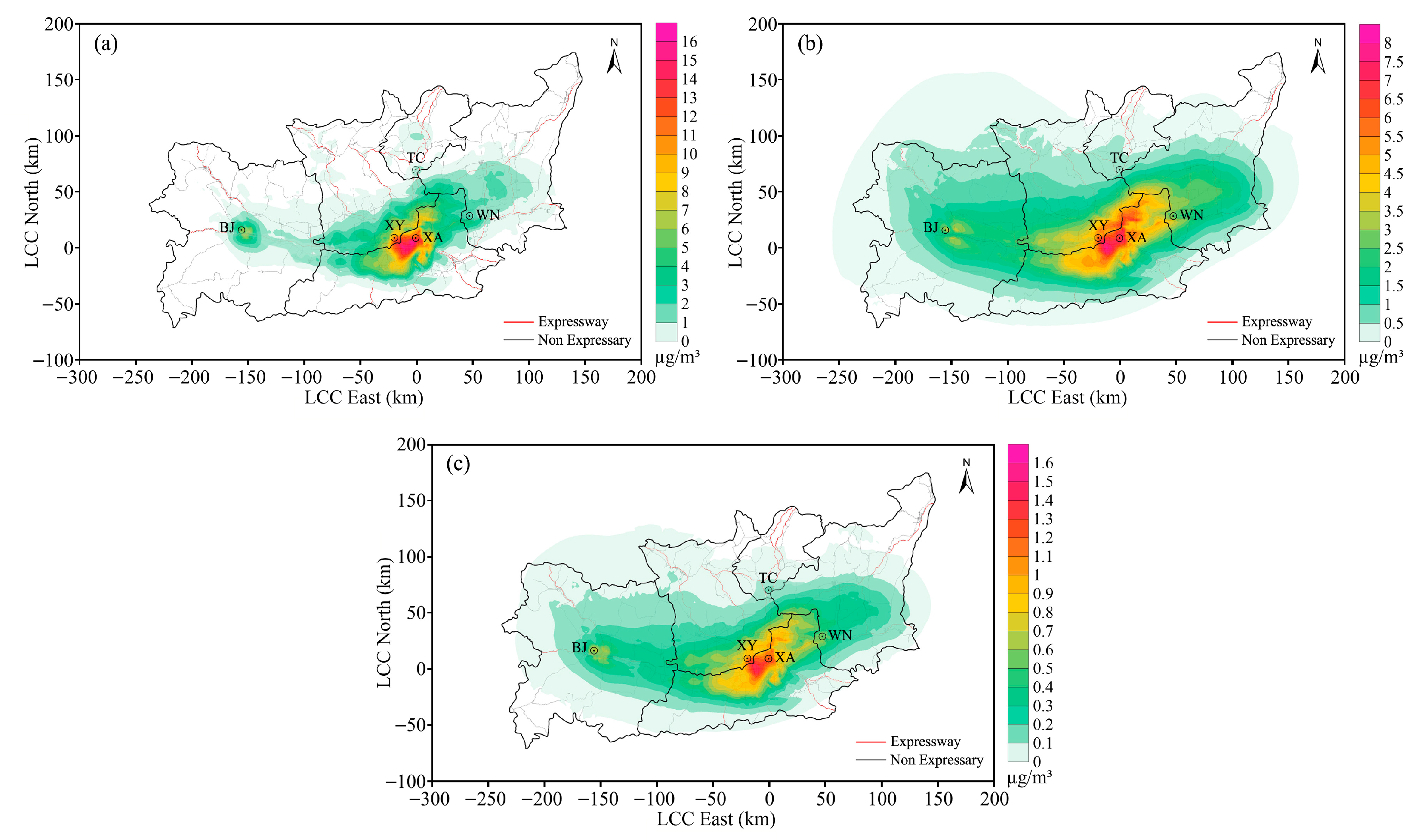
The spatial distribution characteristics of the PM2.5 concentration from vehicles in the GZP in winter are crucial for effectively guiding regional haze control efforts. This study calculated the spatial distribution of the hourly average near-surface concentrations of primary PM2.5, SIA, and SOA from vehicles in the GZP in January 2019, as shown in Figure 5.
The spatial distribution of the primary PM2.5 concentration exhibited a decreasing trend from the five urban centers towards the surrounding suburbs, with relatively high concentrations occurring in the dense areas of urban road networks and near the expressway in the suburbs. This indicated that the spatial distribution of the primary PM2.5 concentration from vehicles in the GZP was consistent with the spatial distribution of its emissions, and the primary PM2.5 emitted by vehicles in this region in winter was not easily dispersed. In the urban area, the primary PM2.5 concentration was the highest in the southwest of the main urban area of XA and the southeast of the main urban area of XY, and the maximum primary PM2.5 concentration was 17.62 µg/m3. In the suburbs, the primary PM2.5 concentration near the expressway was markedly higher than that in the surrounding areas. The spatial distribution trends of the SIA concentration and SOA concentration from vehicles were similar, both of which gradually decreased from the southwest of the main urban area of XA to the periphery, and the distribution characteristics along the road network were not distinct. The maximum hourly average concentrations of SIA and SOA were 8.59 and 1.51 µg/m3, respectively. The concentration distribution range of SIA and SNA was significantly larger than that of primary PM2.5, and both SIA and SNA had been dispersed over a large area in the upper part of the Loess Plateau. At the same time, the concentration of SIA and SNA had an obvious dispersion trend to the east of WN and the west of BJ, implying that the dispersion of secondary PM2.5 in winter was significantly influenced by the dominant northeast wind and the secondary prevailing southwest wind (see Figure 3).
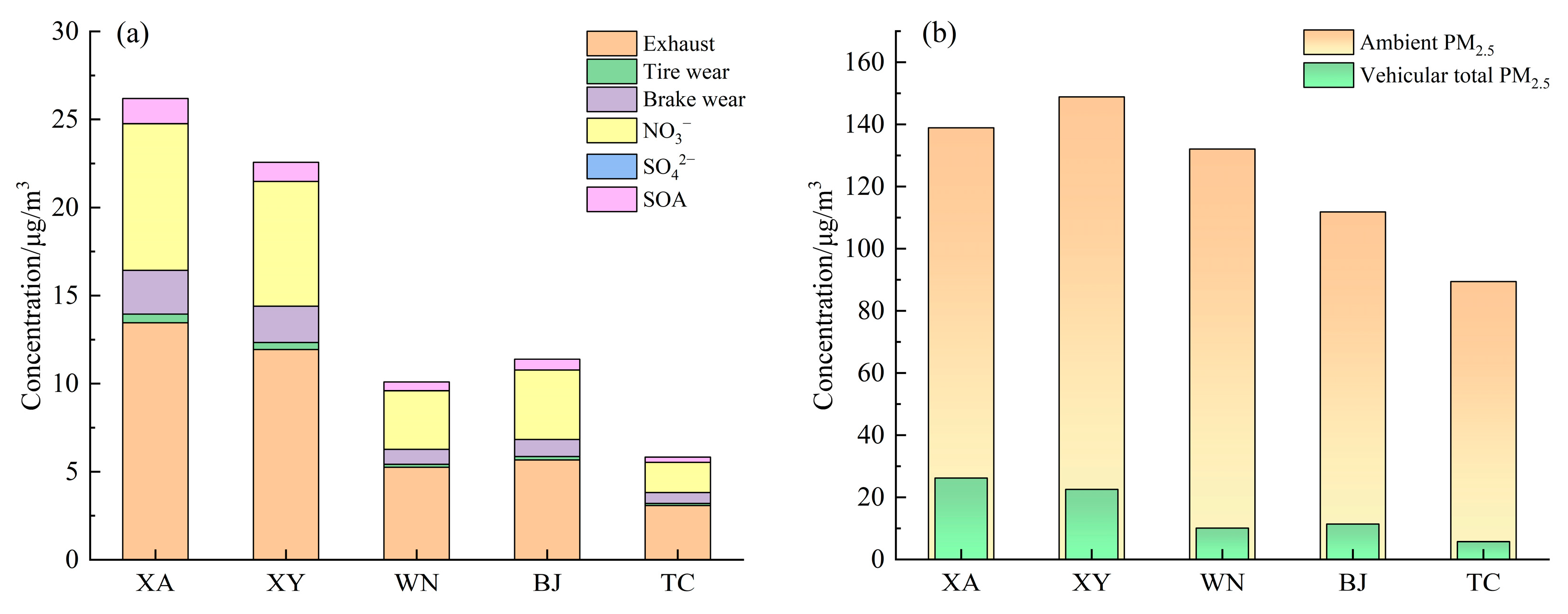
For the purpose of exploring the contribution of different emission pathways of vehicles to the total PM2.5 concentration from vehicles and the contribution of the total PM2.5 concentration to the near-surface ambient PM2.5 concentration, the concentration values extracted from the locations of 33 state-controlled air quality monitoring sites in the concentration field were used as the concentration representative of each city (see Figure 1). Figure 6 shows the total PM2.5 concentration from vehicles and its contribution to the ambient PM2.5 concentration in cities in the GZP in January 2019. The total PM2.5 concentration from vehicles was the highest in XA and the lowest in TC, with values of 26.19 and 5.71 µg/m3, respectively. Although the emissions of primary PM2.5 and gaseous precursors of secondary PM2.5 from vehicles in WN were higher than those in XA and BJ, the total PM2.5 concentration in WN was lower than that in XY and BJ. Among the contributions of different emission pathways of vehicles to the total PM2.5 concentration in five cities, exhaust emissions contributed the most, followed by secondary NO3, brake wear, SOA, tire wear, and secondary SO42−, accounting for 49.78–53.96%, 30.01–34.64%, 8.42–9.49%, 4.78–5.46%, 1.67–1.88%, and 0.02–0.03%, respectively. For the whole Guanzhong region, their average contributions to the total PM2.5 concentration from vehicles were 51.77%, 32.03%, 9.22%, 5.14%, 1.83%, and 0.02%, respectively. It can be seen that the contribution of non-exhaust emissions and secondary conversion to the total PM2.5 concentration reached about 50%. The secondary NO3 was the second largest contributor to the total PM2.5 concentration, which was mainly related to the large amount of NOx emissions and the low ambient temperature. The lower ambient temperature (<15 °C) in winter is conducive to promoting the gas-particle conversion of secondary NO3 [57,58]. For each city, the contributions of vehicle emissions to the ambient PM2.5 concentration in XA, XY, BJ, WN, and TC were 18.86%, 15.16%, 10.19%, 7.65%, and 6.38%, respectively. When only considering the contribution of vehicle exhaust emissions to the ambient PM2.5 concentration in XA, its contribution rate was 9.69%, which was close to the conclusion of Cao and Cui [59].

3.4. Inter-City Transport of PM2.5 Concentrations

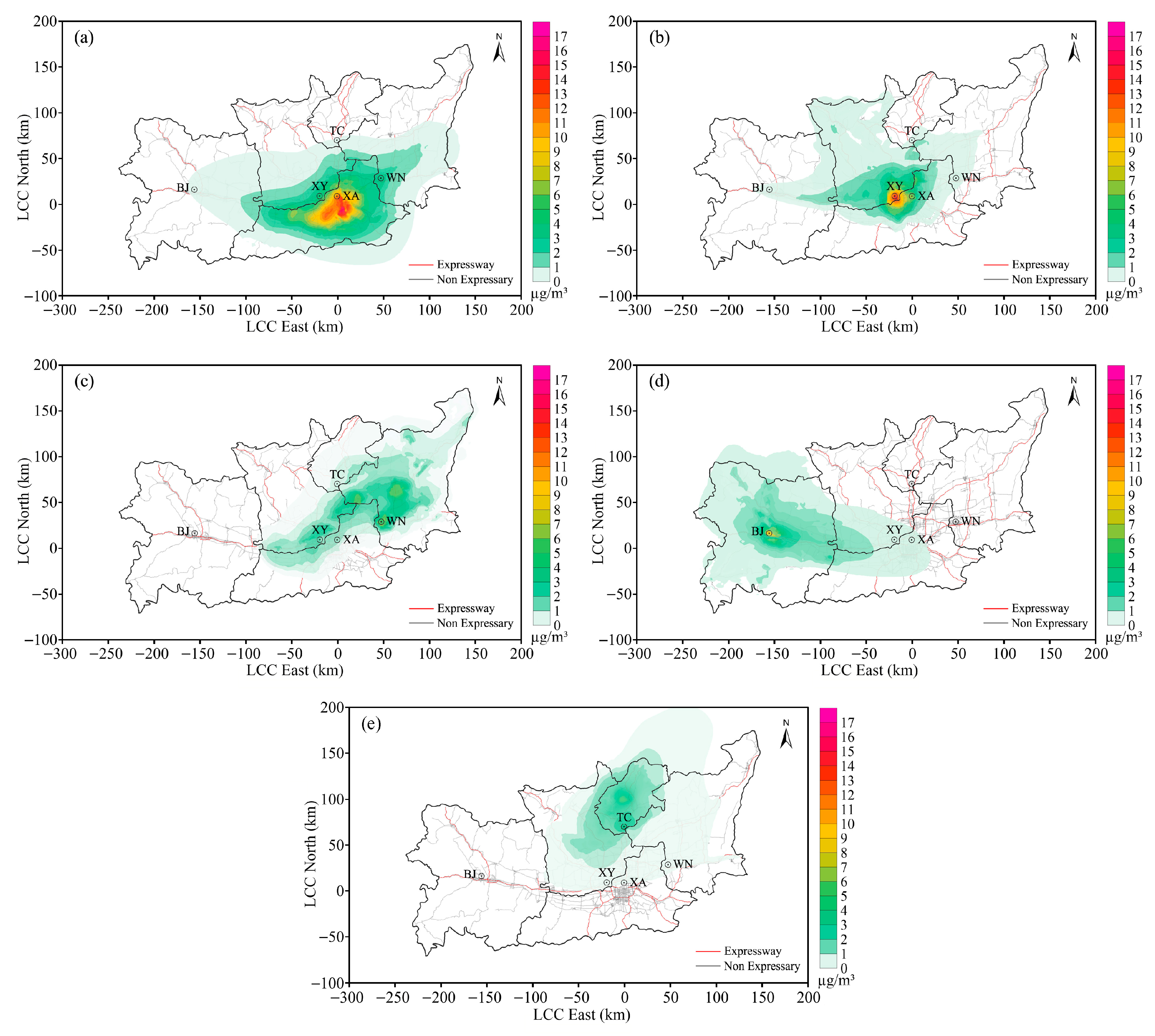
To determine the inter-city transport extent of PM2.5 from vehicles in the GZP, this study separately calculated the dispersion of PM2.5 emitted by vehicles in each city in January 2019 under the same meteorological conditions, as shown in Figure 7. The concentration distribution range of PM2.5 from XA was the largest, and it was transported to the other four cities, especially to its neighboring XY and WN. The high concentration of PM2.5 from vehicles in XY was mainly concentrated in the middle of the main urban area and the junction with the main urban area of XA. Due to the proximity of the main urban areas of XY and XA, the range and amount of PM2.5 mutual transport between the two cities were relatively large. The high concentration of PM2.5 emitted by vehicles in WN was scattered, mainly in its main urban area, as well as in the western and central counties with dense road networks. Under the influence of the prevailing northeast wind in winter, the PM2.5 concentration had an obvious dispersion trend to XY and XA. Affected by the secondary prevailing southwest wind in winter, the PM2.5 from vehicles in BJ was transported to the main urban areas of XY and XA in the northeast direction, but not to TC and WN. Because most areas of TC belong to the Loess Plateau and the terrain is relatively high, the PM2.5 from other cities was transported to the city in a small scope, and the transported area was mainly concentrated in the main urban area with low terrain. The PM2.5 emitted by vehicles in TC was mainly transported to its neighboring city of XY.
Figure 8 shows the transport contribution of PM2.5 emitted by vehicles between cities in the GZP and the proportion of transport components. It can be observed that local emission was the main source of near-surface PM2.5 concentration from vehicles in various cities, and the local emission in BJ contributed the most, accounting for 83%. For all cities, inter-city transport contributed 32.66% of the total PM2.5 concentration from vehicles on average. The PM2.5 concentration in XA and XY was not only from their own local emissions, but also from the transport of the other four cities in the GZP. In particular, the vehicle emissions in XY and XA were the largest transport sources of near-surface PM2.5 concentration to each other in winter, and their transport contributions were comparable, both of which were about 22.5%. The transport of vehicle emissions from XA contributed the most to the near-surface PM2.5 concentration in WN, followed by XY, accounting for 30% and 10%, respectively. The PM2.5 transport to BJ was only from XA and XY, and their transport contribution was 8% and 9%, respectively. The transport contribution from XY and WN to TC was similar, and both were greater than that from XA. It is evident that the transport of PM2.5 emitted by vehicles between cities was obvious in the GZP. Among the components of PM2.5 transported in each city, SIA was the most transported, followed by primary PM2.5 and SOA, accounting for 13–29%, 3–16%, and 1–3%, respectively.

4. Conclusions

In this study, based on the MOVES model and field research, we calculated the emission inventory of SO2, NOx, VOCs, and primary PM2.5 from vehicles in the GZP in January 2019. The WRF/CALPUFF modeling system was utilized to simulate the spatial distribution of primary PM2.5, SIA, and SOA concentrations from vehicles in the GZP, and further quantified the contribution of vehicles to near-surface ambient PM2.5 concentrations. In addition, the inter-city transport of PM2.5 emitted by vehicles among cities in the GZP was also estimated. The main conclusions are as follows:
The meteorological simulation results of the WRF/CALMET model in this study were found to be sufficiently reliable by comparing them with observational data. In the spatial distribution of the PM2.5 concentration emitted by vehicles near the ground in winter, primary PM2.5 was not easily dispersed, and its concentration distribution was highly correlated with the density of the road network, while SIA and SOA were more likely to be dispersed, with a wide range of concentration distribution, and their dispersion was significantly affected by the wind direction. The maximum hourly average concentrations of primary PM2.5, SIA, and SOA all occurred in the southwest of the main urban area of XA and the southeast of the main urban area of XY, with values of about 18, 9, and 2 µg/m3, respectively. Regarding the contribution to the PM2.5 concentration, the contribution of exhaust emission, secondary NO3, brake wear, SOA, and tire wear to the total PM2.5 concentration from vehicles in the GZP were about 52%, 32%, 9%, 5%, and 2%, respectively, and the contribution of total PM2.5 from vehicles to the ambient PM2.5 concentration was the largest in XA, accounting for about 19%. For the inter-city transport of PM2.5 emitted by vehicles, the range and amount of transport were largest between XY and XA. Although the near-surface concentration of PM2.5 from vehicles in different cities was mainly due to local emissions, the external transport could not be ignored, and the contribution of transport to the total PM2.5 concentration from vehicles in WN and TC reached about 42% and 40%, respectively. Among the components of PM2.5 transported in each city, SIA was the most abundant, followed by primary PM2.5, and SOA was the least. Consequently, it should be considered to develop a collaborative control plan for pollutants in urban agglomerations. The reduction in primary and secondary PM2.5 emissions from vehicles should receive key attention to improve regional air quality.
It is worth noting that the above analysis of spatial distribution and inter-city transport of PM2.5 concentrations from vehicles is not entirely accurate due to the limitations of the emissions inventory (our source inventory does not include the re-suspended road dust caused by vehicles), but it could help us to understand the dispersion and transport characteristics of pollutants emitted by near-surface sources over complex terrain.

Author Contributions

Conceptualization, P.L.; methodology, A.T.; software, G.L.; validation, S.D.; formal analysis, P.L.; investigation, P.L. and A.T.; resources, G.L. and J.L.; data curation, G.L.; writing—original draft preparation, P.L.; writing—review and editing, S.D. and A.T.; visualization, G.L.; funding acquisition, J.L. All authors have read and agreed to the published version of the manuscript.

Funding

This research was funded by the Key Research and Development Project of Shaanxi Province (No. 2021ZDLSF-05-07), and the Foundation of Science and Technology Coordinating Innovative Engineering Projects of Shaanxi Province (No. 2016KTZDSF-02-01).

Institutional Review Board Statement

Not applicable.

Informed Consent Statement

Not applicable.

Data Availability Statement

Data are contained within the article.

Acknowledgments

The modeling simulations were carried out on the supercomputer provided by Chang’an University.

Conflicts of Interest

The authors declare no conflict of interest.

References

  1. Chen, L.; Zhang, J.; You, Y. Air pollution, environmental perceptions, and citizen satisfaction: A mediation analysis. Environ. Res. 2020, 184, 109287. [Google Scholar] [CrossRef] [PubMed]
  2. Pu, S.; Shao, Z.; Fang, M.; Yang, L.; Liu, R.; Bi, J.; Ma, Z. Spatial distribution of the public’s risk perception for air pollution: A nationwide study in China. Sci. Total Environ. 2019, 655, 454–462. [Google Scholar] [CrossRef] [PubMed]
  3. Gao, S.; Yu, J.; Yang, W.; Qu, F.; Chen, L.; Sun, Y.; Zhang, H.; Mao, J.; Zhao, H.; Azzi, M.; et al. Background concentration of atmospheric PM2.5 in the Beijing-Tianjin-Hebei urban agglomeration: Levels, variation trends, and influences of meteorology and emission. Atmos. Pollut. Res. 2022, 13, 101583. [Google Scholar] [CrossRef]
  4. Ding, Y.; Zhang, M.; Chen, S.; Wang, W.; Nie, R. The environmental Kuznets curve for PM2.5 pollution in Beijing-Tianjin-Hebei region of China: A spatial panel data approach. J. Cleaner Prod. 2019, 220, 984–994. [Google Scholar] [CrossRef]
  5. He, Y.; Lin, K.; Liao, N.; Chen, Z.; Rao, J. Exploring the spatial effects and influencing factors of PM2.5 concentration in the Yangtze River Delta Urban Agglomerations of China. Atmos. Environ. 2022, 268, 118805. [Google Scholar] [CrossRef]
  6. Ming, L.; Jin, L.; Li, J.; Fu, P.; Yang, W.; Liu, D.; Zhang, G.; Wang, Z.; Li, X. PM2.5 in the Yangtze River Delta, China: Chemical compositions, seasonal variations, and regional pollution events. Environ. Pollut. 2017, 223, 200–212. [Google Scholar] [CrossRef] [PubMed]
  7. Feng, T.; Bei, N.; Zhao, S.; Wu, J.; Li, X.; Zhang, T.; Cao, J.; Zhou, W.; Li, G. Wintertime nitrate formation during haze days in the Guanzhong basin, China: A case study. Environ. Pollut. 2018, 243, 1057–1067. [Google Scholar] [CrossRef]
  8. Wei, N.; Wang, N.; Huang, X.; Liu, P.; Chen, L. The effects of terrain and atmospheric dynamics on cold season heavy haze in the Guanzhong Basin of China. Atmos. Pollut. Res. 2020, 11, 1805–1819. [Google Scholar] [CrossRef]
  9. Niu, X.; Cao, J.; Shen, Z.; Ho, S.S.H.; Tie, X.; Zhao, S.; Xu, H.; Zhang, T.; Huang, R. PM2.5 from the Guanzhong Plain: Chemical composition and implications for emission reductions. Atmos. Environ. 2016, 147, 458–469. [Google Scholar] [CrossRef]
  10. World Health Organization (WHO). Ambient (Outdoor) Air Pollution. Available online: https://www.who.int/news-room/fact-sheets/detail/ambient-(outdoor)-air-quality-and-health (accessed on 26 September 2023).
  11. Chinese State Council (CSC) of the People’s Republic of China. Air Pollution Prevention and Control Action Plan. Available online: https://www.gov.cn/gongbao/content/2013/content_2496394.htm (accessed on 2 October 2023).
  12. Cai, S.; Wang, Y.; Zhao, B.; Wang, S.; Chang, X.; Hao, J. The impact of the “air pollution prevention and control action plan” on PM2.5 concentrations in Jing-Jin-Ji region during 2012–2020. Sci. Total Environ. 2017, 580, 197–209. [Google Scholar] [CrossRef]
  13. Ministry of Ecology and Environment (MEE) of the People’s Republic of China. Work Plan for Air Pollution Prevention and Control in Beijing, Tianjin and Hebei and Surrounding Areas in. 2017. Available online: https://www.mee.gov.cn/gkml/hbb/bwj/201708/t20170824_420330.htm (accessed on 5 October 2023).
  14. Ministry of Ecology and Environment (MEE) of the People’s Republic of China. China Mobile Source Environmental Management Annual Report. Available online: https://www.mee.gov.cn/hjzl/sthjzk/ydyhjgl/202212/W020221207387013521948.pdf (accessed on 15 September 2023).
  15. Luo, Z.; Wang, Y.; Lv, Z.; He, T.; Zhao, J.; Wang, Y.; Gao, F.; Zhang, Z.; Liu, H. Impacts of vehicle emission on air quality and human health in China. Sci. Total Environ. 2022, 813, 152655. [Google Scholar] [CrossRef] [PubMed]
  16. Goel, R.; Guttikunda, S.K. Evolution of on-road vehicle exhaust emissions in Delhi. Atmos. Environ. 2015, 105, 78–90. [Google Scholar] [CrossRef]
  17. Liu, J.; Zheng, B. A Simulation Study on the Influence of Street Tree Configuration on Fine Particulate Matter (PM2.5) Concentration in Street Canyons. Forests 2023, 14, 1550. [Google Scholar] [CrossRef]
  18. Craig, K.J.; Baringer, L.M.; Chang, S.; McCarthy, M.C.; Bai, S.; Seagram, A.F.; Ravi, V.; Landsberg, K.; Eisinger, D.S. Modeled and measured near-road PM2.5 concentrations: Indianapolis and Providence cases. Atmos. Environ. 2020, 240, 117775. [Google Scholar] [CrossRef]
  19. Lu, D.; He, H.; Wang, Z.; Zhao, H.; Peng, Z. Impact of urban viaducts on the vertical distribution of fine particles in street canyons. Atmos. Pollut. Res. 2023, 14, 101726. [Google Scholar] [CrossRef]
  20. Nagendra, S.S.; Diya, M.; Chithra, V.S.; Menon, J.S.; Peter, A.E. Characteristics of air pollutants at near and far field regions of a national highway located at an industrial complex. Transp. Res. Part D 2016, 48, 1–13. [Google Scholar] [CrossRef]
  21. Salva, J.; Vanek, M.; Schwarz, M.; Gajtanska, M.; Tonhauzer, P.; Ďuricová, A. An Assessment of the On-Road Mobile Sources Contribution to Particulate Matter Air Pollution by AERMOD Dispersion Model. Sustainability 2021, 13, 12748. [Google Scholar] [CrossRef]
  22. Wang, B.; Wu, J.; Xu, X.; Li, Y. Hourly population exposure index for PM2.5 in urban street canyons. Urban Clim. 2022, 45, 101242. [Google Scholar] [CrossRef]
  23. Tong, R.; Liu, J.; Wang, W.; Fang, Y. Health effects of PM2.5 emissions from on-road vehicles during weekdays and weekends in Beijing, China. Atmos. Environ. 2020, 223, 117258. [Google Scholar] [CrossRef]
  24. Samuelsen, S.; Zhu, S.; Kinnon, M.M.; Yang, O.K.; Dabdub, D.; Brouwer, J. An episodic assessment of vehicle emission regulations on saving lives in California. Environ. Sci. Technol. 2020, 55, 547–552. [Google Scholar] [CrossRef]
  25. Camilleri, S.F.; Montgomery, A.; Visa, M.A.; Schnell, J.L.; Adelman, Z.E.; Janssen, M.; Grubert, E.A.; Anenberg, S.C.; Horton, D.E. Air quality, health and equity implications of electrifying heavy-duty vehicles. Nat. Sustain. 2023. [Google Scholar] [CrossRef]
  26. Joo, S.; Oh, C.; Lee, S.; Lee, G. Assessing the impact of traffic crashes on near freeway air quality. Transp. Res. Part D 2017, 57, 64–73. [Google Scholar] [CrossRef]
  27. Filigrana, P.; Milando, C.; Batterman, S.; Levy, J.I.; Mukherjee, B.; Adar, S.D. Spatiotemporal variations in traffic activity and their influence on air pollution levels in communities near highways. Atmos. Environ. 2020, 242, 117758. [Google Scholar] [CrossRef]
  28. Lu, P.; Deng, S.; Li, G.; Li, J.; Xu, K.; Lu, Z. Spatial Distribution of Primary and Secondary PM2.5 Concentrations Emitted by Vehicles in the Guanzhong Plain, China. Atmosphere 2022, 13, 347. [Google Scholar] [CrossRef]
  29. Charabi, Y.; Abdul-Wahab, S.; Al-Rawas, G.; Al-Wardy, M.; Fadlallah, S. Investigating the impact of monsoon season on the dispersion of pollutants emitted from vehicles: A case study of Salalah City, Sultanate of Oman. Transp. Res. Part D 2018, 59, 108–120. [Google Scholar] [CrossRef]
  30. Lee, H.D.; Yoo, J.W.; Kang, M.K.; Kang, J.S.; Jung, J.H.; Oh, K.J. Evaluation of concentrations and source contribution of PM10 and SO2 emitted from industrial complexes in Ulsan, Korea: Interfacing of the WRF–CALPUFF modeling tools. Atmos. Pollut. Res. 2014, 5, 664–676. [Google Scholar] [CrossRef]
  31. Guo, D.; Wang, R.; Zhao, P. Spatial distribution and source contributions of PM2.5 concentrations in Jincheng, China. Atmos. Pollut. Res. 2020, 11, 1281–1289. [Google Scholar] [CrossRef]
  32. Hooftman, N.; Oliveira, L.; Messagie, M.; Coosemans, T.; Van Mierlo, J. Environmental Analysis of Petrol, Diesel and Electric Passenger Cars in a Belgian Urban Setting. Energies 2016, 9, 84. [Google Scholar] [CrossRef]
  33. Zhang, N.N.; Ma, F.; Qin, C.B.; Li, Y.F. Spatiotemporal trends in PM2.5 levels from 2013 to 2017 and regional demarcations for joint prevention and control of atmospheric pollution in China. Chemosphere 2018, 210, 1176–1184. [Google Scholar] [CrossRef]
  34. Khuzestani, R.B.; Schauer, J.J.; Wei, Y.; Zhang, L.; Cai, T.; Zhang, Y.; Zhang, Y. Quantification of the sources of long-range transport of PM2.5 pollution in the Ordos region, Inner Mongolia, China. Environ. Pollut. 2017, 229, 1019–1031. [Google Scholar] [CrossRef]
  35. Song, Y.; Li, Z.; Yang, T.; Xia, Q. Does the expansion of the joint prevention and control area improve the air quality?—Evidence from China’s Jing-Jin-Ji region and surrounding areas. Sci. Total Environ. 2020, 706, 136034. [Google Scholar] [CrossRef] [PubMed]
  36. Chang, X.; Wang, S.; Zhao, B.; Xing, J.; Liu, X.; Wei, L.; Song, Y.; Wu, W.; Cai, S.; Zheng, H.; et al. Contributions of inter-city and regional transport to PM2.5 concentrations in the Beijing-Tianjin-Hebei region and its implications on regional joint air pollution control. Sci. Total Environ. 2019, 660, 1191–1200. [Google Scholar] [CrossRef] [PubMed]
  37. He, J.; Zhang, L.; Yao, Z.; Che, H.; Gong, S.; Wang, M.; Zhao, M.; Jing, B. Source apportionment of particulate matter based on 448 numerical simulation during a severe pollution period in Tangshan, North China. Environ. Pollut. 2020, 266, 115133. [Google Scholar] [CrossRef] [PubMed]
  38. Ministry of Civil Affairs (MCA) of the People’s Republic of China. National Administrative Division Information Query Platform. Available online: http://xzqh.mca.gov.cn/map (accessed on 25 September 2023).
  39. Liu, R.; He, H.D.; Zhang, Z.; Wu, C.L.; Yang, J.M.; Zhu, X.H.; Peng, Z.R. Integrated MOVES model and machine learning method for prediction of CO2 and NO from light-duty gasoline vehicle. J. Clean Prod. 2023, 422, 138612. [Google Scholar] [CrossRef]
  40. Perugu, H. Emission modelling of light-duty vehicles in India using the revamped VSP-based MOVES model: The case study of Hyderabad. Transp. Res. Part D 2018, 68, 150–163. [Google Scholar] [CrossRef]
  41. Hong, Z.L.; Zimmerman, N. Air quality and greenhouse gas implications of autonomous vehicles in Vancouver, Canada. Transp. Res. Part D 2021, 90, 102676. [Google Scholar] [CrossRef]
  42. Li, X.; Hussain, S.A.; Sobri, S.; Said, M.S.M. Overviewing the air quality models on air pollution in Sichuan Basin, China. Chemosphere 2021, 271, 129502. [Google Scholar] [CrossRef]
  43. Abdul-Wahab, S.; Sappurd, A.; Al-Damkhi, A. Application of California Puff (CALPUFF) model: A case study for Oman. Clean Technol. Environ. Policy 2011, 13, 177–189. [Google Scholar] [CrossRef]
  44. Holnicki, P.; Kałuszko, A.; Trapp, W. An urban scale application and validation of the CALPUFF model. Atmos. Pollut. Res. 2016, 7, 393–402. [Google Scholar] [CrossRef]
  45. Huang, D.; Guo, H. Dispersion modeling of odour, gases, and respirable dust using AERMOD for poultry and dairy barns in the Canadian Prairies. Sci. Total Environ. 2019, 690, 620–628. [Google Scholar] [CrossRef]
  46. Foley, K.M.; Pouliot, G.A.; Eyth, A.; Aldridge, M.F.; Allen, C.; Appel, K.W.; Bash, J.O.; Beardsley, M.; Beidler, J.; Choi, D.; et al. 2002–2017 anthropogenic emissions data for air quality modeling over the United States. Data Brief 2023, 47, 109022. [Google Scholar] [CrossRef]
  47. Meroni, A.; Pirovano, G.; Gilardoni, S.; Lonati, G.; Colombi, C.; Gianelle, V.; Paglione, M.; Polluzzi, V.; Riva, G.M.; Toppetti, A. Investigating the role of chemical and physical processes on organic aerosol modelling with CAMx in the Po Valley during a winter episode. Atmos. Environ. 2017, 171, 126–142. [Google Scholar] [CrossRef]
  48. Bezyk, Y.; Oshurok, D.; Dorodnikov, M.; Sówka, I. Evaluation of the CALPUFF model performance for the estimation of the urban ecosystem CO2 flux. Atmos. Pollut. Res. 2020, 12, 260–277. [Google Scholar] [CrossRef]
  49. Otero-Pregigueiro, D.; Fernández-Olmo, I. Use of CALPUFF to predict airborne Mn levels at schools in an urban area impacted by a nearby manganese alloy plant. Environ. Int. 2018, 119, 455–465. [Google Scholar] [CrossRef]
  50. Scire, J.S.; Strimaitis, D.G.; Yamartino, R.J. A User’s Guide for the CALPUFF Dispersion Model; Version 7.3.2; Exponent Inc.: Concord, MA, USA, 2019; Available online: https://www.src.com/calpuff/download/CALPUFF_v7_UserGuide_Addendum.pdf (accessed on 7 September 2023).
  51. Kia, S.; Flesch, T.K.; Freeman, B.S.; Aliabadi, A.A. Calculating gas emissions from open-pit mines using inverse dispersion modelling: A numerical evaluation using CALPUFF and CFD-LS. J. Wind Eng. Ind. Aero. 2022, 226, 105046. [Google Scholar] [CrossRef]
  52. Tan, R.; Guo, S.; Lu, S.; Wang, H.; Zhu, W.; Yu, Y.; Tang, R.; Shen, R.; Song, K.; Lv, D.; et al. Characteristics and Secondary Organic Aerosol Formation of Volatile Organic Compounds from Vehicle and Cooking Emissions. Atmosphere 2023, 14, 806. [Google Scholar] [CrossRef]
  53. Huang, C.; Wang, H.L.; Li, L.; Wang, Q.; Lu, Q.; de Gouw, J.A.; Zhou, M.; Jing, S.A.; Lu, J.; Chen, C.H. VOC species and emission inventory from vehicles and their SOA formation potentials estimation in Shanghai, China. Atmos. Chem. Phys. 2015, 15, 7977–8015. [Google Scholar] [CrossRef]
  54. Wu, C.; Wang, G.; Li, J.; Li, J.; Cao, C.; Ge, S.; Xie, Y.; Chen, J.; Liu, S.; Du, W.; et al. Non-agricultural sources dominate the atmospheric NH3 in Xi’an, a megacity in the semi-arid region of China. Sci. Total Environ. 2020, 722, 137756. [Google Scholar] [CrossRef]
  55. Wu, H.; Zhang, Y.; Yu, Q.; Ma, W. Application of an integrated Weather Research and Forecasting (WRF)/CALPUFF modeling tool for source apportionment of atmospheric pollutants for air quality management: A case study in the urban area of Benxi, China. J. Air Waste Manag. Assoc. 2018, 68, 347–368. [Google Scholar] [CrossRef]
  56. Levy, I.; Mahrer, Y.; Dayan, U. Coastal and synoptic recirculation affecting air pollutants dispersion: A numerical study. Atmos. Environ. 2009, 43, 1991–1999. [Google Scholar] [CrossRef]
  57. Xu, J.S.; Xu, M.X.; Snape, C.; He, J.; Behera, S.N.; Xu, H.H.; Ji, D.S.; Wang, C.J.; Yu, H.; Xiao, H.; et al. Temporal and spatial variation in major ion chemistry and source identification of secondary inorganic aerosols in Northern Zhejiang Province, China. Chemosphere 2017, 179, 316–330. [Google Scholar] [CrossRef] [PubMed]
  58. Feng, J.; Yu, H.; Mi, K.; Su, X.; Li, Y.; Li, Q.; Sun, J. One year study of PM2.5 in Xinxiang city, North China: Seasonal characteristics, climate impact and source. Ecotox. Environ. Saf. 2018, 154, 75–83. [Google Scholar] [CrossRef] [PubMed]
  59. Cao, J.J.; Cui, L. Current status, characteristics and causes of particulate air pollution in the Fenwei Plain, China: A review. J. Geophys. Res. Atmos. 2021, 126, e2020JD034472. [Google Scholar] [CrossRef]
Figure 1. The location and topography of the Guanzhong Plain (GZP) and the simulated domains.
Atmosphere 14 01748 g001
Figure 2. The allocation results of line sources and area sources.
Atmosphere 14 01748 g002
Figure 3. The wind roses obtained by observation (a) and simulation (b) in the GZP in January 2019.
Atmosphere 14 01748 g003
Figure 4. The time series of simulated and observed daily average temperatures (a), relative humidity (b), and wind speeds (c) at meteorological sites in the GZP in January 2019.
Atmosphere 14 01748 g004
Figure 5. The spatial distribution of the hourly average concentrations of primary PM2.5 (a), secondary inorganic aerosols (SIA) (b), and secondary organic aerosols (SOA) (c) from vehicles in the GZP in January 2019.
Atmosphere 14 01748 g005
Figure 6. The total PM2.5 concentration from vehicles (a) and its contribution to the ambient PM2.5 concentration (b) in cities in the GZP in January 2019.
Atmosphere 14 01748 g006
Figure 7. The spatial distribution of total PM2.5 concentration from vehicles in Xi’an (a), Xianyang (b), Weinan (c), Baoji (d), and Tongchuan (e) in January 2019.
Atmosphere 14 01748 g007
Figure 8. The transport contribution of PM2.5 emitted by vehicles between cities in the GZP (a) and the proportion of transport components (b) in January 2019.
Atmosphere 14 01748 g008
Table 1. The parameterization schemes for WRF.
Parameterization SchemeScheme Name
Solar radiation schemeDudhia
Longwave and shortwave radiation schemeRRTM
Microphysics process schemeWSM6
Boundary layer schemeACM2
Surface layer schemeObukhov
Land surface schemeNoah-MP
Cumulus convection schemeKain-Fritsch
Table 2. The main parameters set in CALPUFF.
Model ParameterParameter Settings
Map projectionLambert Conic Conformal
Domain size500 km × 250 km
Horizontal and vertical diffusionGaussian
Terrain adjustmentISC terrain adjustment scheme
Plume riseBriggs Plume Rise
Building downwashISC method
Dispersion optionTurbulence computed from micrometeorology
Chemical transformationRIVAD + ISORROPIA + CalTechSOA
DepositionVertical Structure and Mass Depletion/Resistance Deposition Model
Initial and boundary conditionsDefault
Table 3. Emission inventory of SO2, NOx, VOCs, and primary PM2.5 from vehicles in each city of GZP in January 2019 (t).
CitySO2NOxVOCsPrimary PM2.5
Exhaust EmissionBrake WearTire Wear
XA10.033292.731111.49125.4430.026.07
WN3.481318.70499.6690.317.351.41
XY1.96752.14262.0528.585.310.97
BJ1.75612.59434.0123.702.990.63
TC0.70306.66107.1720.331.890.35
GZP17.926282.822414.38288.3647.569.43
Disclaimer/Publisher’s Note: The statements, opinions and data contained in all publications are solely those of the individual author(s) and contributor(s) and not of MDPI and/or the editor(s). MDPI and/or the editor(s) disclaim responsibility for any injury to people or property resulting from any ideas, methods, instructions or products referred to in the content.