Abstract
In the present work, the main methodologies used to reconstruct wind fields in the U-SPACE have been analyzed. The SESAR U-SPACE program aims to develop an Unmanned Traffic Management system with a progressive introduction of procedures and services designed to support secure access to the air space for a large number of drones. Some of these techniques were originally developed for reconstruction at high altitudes, but successively adapted to treat different heights. A common approach to all techniques is to approximate the probabilistic distribution of wind speed over time with some parametric models, apply spatial interpolation to the parameters and then read the predicted value. The approaches are based on the fact that modern aircraft are equipped with automatic systems. Moreover, the proposed concepts demonstrated the possibility of using drones as a large network to complement the current network of sensors. The methods can serve the micro-scale weather forecasts and the collection of information necessary for the definition of the flight plan of drones in urban contexts. Existing limitations in the applications of wind field reconstruction, related to the fact that estimations can be produced only if a sufficient number of drones are already flying, could be mitigated using data provided by Numerical Weather Prediction models (NWPs). The coupling of methodologies used to reconstruct wind fields with an NWP will ensure that estimations can be produced in any geographical area.
1. Introduction
The concept of U-SPACE has been introduced in order to support commercial operations with drones, especially those characterized by great complexity and automation [1]. The SESAR (Single European Sky ATM Research) U-SPACE program [2] aims to develop a UTM (Unmanned Traffic Management) system, with a progressive introduction of procedures and services designed to support a secure efficient and protected access to the air space for a large number of drones. In this view, the need arose to develop specific services for drone operation in urban contexts, in particular with respect to the availability of local weather forecasts (hazard detection and nowcasting) and information for navigation in high-density population areas, since meteorological conditions could have a strong impact on the drone flight. “Micro-weather management” [3] in particular is considered one of the enabling factors for operations beyond the line of sight in an urban context, such as to have an urgent nature for the first implementation solutions of the national U-SPACE.
Within this framework, the Italian Aerospace Research Center (CIRA, Italy) is carrying out the internal project EDUS “Infrastrutture di elaborazione dati locali per U-SPACE”. The project focuses on the development and validation of operating platform demonstrators serving the micro-scale weather forecasts and the collection of information necessary for the definition of the flight plan of the drones in urban contexts. These platforms will be built upon the Meteo Service Center already existing at CIRA [4], which collects and processes observational and forecast atmospherical data on different time ranges, provided by ground stations, satellite data and Numerical Weather Prediction (NWP) models (in particular, COSMO-LM [5] and ICON [6]). In this perspective, the project exploits basic technologies and tools that are already available and validated in similar operational contexts, providing for an adaptation to the specific development needs of the national U-SPACE. Compared with other meteorological variables, the observational data of wind fields are generally scarce; for this reason, research in this field has become an urgent need to support civil aviation.
The present work contains an analysis of the state of art on methodologies that can be used to estimate winds at low altitudes in urban areas. Some of these techniques were originally developed for reconstruction at high altitudes, but successively they have been adapted to treat different heights. A common approach to all techniques is to approximate the probabilistic distribution of wind speed over time with some parametric models, apply spatial interpolation to the parameters and then read the predicted value. The problem of wind forecasting is deeply felt in the aeronautical field; in fact, several studies (e.g., [7]) have analyzed the effect of errors in wind forecasting on Continuous Descent Operations, concluding that the accurate knowledge of the actual wind conditions is of the utmost importance since about 2/3 of the average error is due to an incorrect wind forecast. In [8], Dalmau et al. combined a nonlinear predictive control model (NMPC) that cyclically updates an aircraft’s optimal trajectory with a wind network through which aircraft and ground systems share observed real-time wind data to improve flight profile prediction. The results showed how the availability of updated wind data allows us to significantly improve the performance of the NMPC, along with significant fuel savings. Limitations in the applications of wind field reconstruction are also related to the fact that estimations can be produced only if a sufficient number of drones is already flying in the area considered; this limitation could be mitigated using data provided by NWPs, which take current observations as input through a process defined data assimilation [9] and produce initial conditions for the meteorological variables, using 3D/4D variational assimilation schemes that are better suited for large spatiotemporal modeling with data from different observation sources. In ref. [10], a digital meteo model (DMET) that combines atmospheric data from several sources into a 4D predictive scenario was presented. It is worth mentioning the nudging data assimilation technique [11], in which partial field measurements are used to control the evolution of a dynamical system and to reconstruct the phase space configuration of the supplied flow.
The following methodologies have been analyzed in the present work (Table 1): the Airborne Wind Estimation Algorithm (AWEA) estimates wind profiles using measurements of wind data taken from nearby aircraft and provides high-fidelity and high-resolution user-tailored wind profiles; the random Fourier features a novel interpolation model that resulted competitive with respect to other statistical interpolation models; the Meteo Particle Model demonstrates the possibility of using drones as a large sensor network to construct a global scale real-time meteorological measurement system; and NWPs take current weather observations as input and deliver weather forecasts by solving the full set of prognostic equations of atmosphere. This paper is organized as follows: in Section 2, Section 3 and Section 4, the mentioned methodologies that can be used to estimate low-altitude winds in urban areas are presented; and Section 5 describes some examples of applications of the Meteo Particle Model (MPM). An introduction to NWP models is provided in Section 6 and, finally, a discussion and the main conclusions are presented in Section 7.

Table 1.
List of the methodologies analyzed in the present work.
2. AWEA—Airborne Wind Estimation Algorithm
Drone operators are generally supported by specific platforms, designed as a decision support system for piloted flight operations capable of transitioning to a decision-making system for fully autonomous flights. Weather data provided by U-SPACE Service Providers through their platforms must be in accordance with the latest EASA (European Union Aviation Safety Agency) regulations.
In order to have a reliable estimation of wind, currently aircraft pilots mainly use bulletin winds and meteorological charts provided, e.g., by the Aviation Weather Center, by EASA, or by specific service providers such as NOAA Rapid Refresh (rapidrefresh.nooa.gov), which are defined on grids at a resolution of about 10 km, generally updated once at hour. On the basis of these charts, pilots insert wind data into the Flight Management System (FMS) to make estimates of the fuel required and flight time. Several studies tried to find new solutions to improve the information quality to provide to the FMS, from a simple profile based on the wind measured onboard to data generated by models. Mondoloni [16] used statistical data and techniques based on the Kalman filter [17] to estimate wind values aimed at the trajectory definition. Other authors used radar tracks to estimate wind fields in the neighborhood of an aircraft and then used the Kalman filter to reduce the effects of measurement noise. Bienert and Fricke [18] proposed a methodology based on a real-time wind uplink for prediction of the arrival time and the optimization of the descent profile, which is able to provide a high-resolution profile, but does not offer a large update frequency. De Prins et al. [19] introduced an enhanced self-spacing algorithm for a three-degree decelerating approach, able to provide only an estimate for a selected area. To build high-resolution wind profiles in real time, de Jong et al. [12] introduced AWEA (Airborne Wind Estimation Algorithm), a new algorithm based on the fact that modern aircraft are equipped with automatic systems (e.g., ADS-B [20]) able to send and receive atmospheric data, allowing the reception of information from vehicles in proximity, in a short time. AWEA builds wind profiles by using the Kalman filter, which extracts the noise components of the measured wind data [21] and assigns smaller weights to measurements that were taken farther in time or at a larger distance from the reference trajectory. Alternative approaches to the Kalman filter are available in the literature, such as the particle filter [22], which recursively updates an estimate of the state and finds the innovations by a sequential Monte Carlo method. This approach is particularly suitable in a non-linear and/or non-Gaussian environment.
This approach has the advantage that all the aircraft collect data and then operate as airborne sensors so that the resolution and the frequency of wind estimate update is increased. In this way, the software packages for the trajectory forecast can use the most recent wind estimates available. AWEA was specifically developed to improve onboard trajectory prediction, but can also be used on the ground for the estimation of an entire wind field [23].
AWEA uses onboard measurements provided by other aircraft to build a wind profile along its own trajectory by using a stochastic model, without using physical laws. All the observations are grouped into intervals of predefined altitudes and then processed through a Kalman filter, even to assign lower weights to those measurements taken at a large distance from the trajectory being considered. Filtered and weighted data are then used to define a wind estimate at each altitude for a short time interval, while the final profile is built using a linear interpolation. The advantage of using aircraft-collected information is that such data are spatially and temporally concentrated around the most crowded tracks and in the maneuver areas of airports. On the other side, the wind estimate accuracy is lower in less crowded areas, but this does not imply severe problems since under these conditions a lower accuracy in the trajectory forecast is acceptable, because in these situations the runway capacity is substantially less than the maximum available capacity.
AWEA can be run onboard or on the ground station: in the first case, it uses its own data and information received from aircraft in the neighborhood, eventually supported by a profile received from the ground station; in the second case, the ground station receives meteorological information to continuously estimate a wind profile representative of the whole Terminal Control Area (TMA). As soon as an aircraft enter the TMA, it receives the last estimated wind profile needed to update the planning of the last descent phase. This methodology is able to create specific profiles tailored to each airplane entering the TMA or create a unique profile. The algorithm works through the following steps:
- Definition of a flight trajectory;
- Generation of a first-attempt solution. It is produced through a standard logarithmic profile [24] starting from a measurement performed onboard.in which the velocity Vw (m/s) changes with the altitude h (m) and depends on the wind velocity Vw0 measured at an assigned height h0. The numerical value of the p exponent is empirically obtained and is equal to 1/7. This power law equation yields a very general approximation of the wind profile in the Planetary Boundary Layer (PBL).
- Kalman filter update at the frequency 1 Hz.
The Kalman filter is composed of five consecutive steps, at each time instant, in the following way:
- (1)
- The filter starts to predict the state estimate x and estimate covariance P.
- (2)
- When new observations are available, they are used to construct the observation model matrix C. The observations determine the measurement noise covariance matrix R too. The coefficients of R depend on Kw, which is a scaling parameter varying between 0 and 1. Kw determines the influence of an observation based on the distance between the measurement and the trajectory at the same altitude.
- (3)
- The innovation covariance matrix S is calculated using the C and R matrices. In this way, the current estimate for the altitude of the observation can be calculated and compared to the measured value to determine the innovation.
- (4)
- The Kalman gain K is determined by using the observation model, the state covariance and innovation covariance matrices.
- (5)
- The innovation is multiplied by the Kalman gain, providing the updated state estimate.
A high uncertainty in the current estimate (high value of P) and good confidence in the accuracy of the measurement (low value of S) implies a high value of the Kalman gain, which assigns a large weight to the incoming observation. On the contrary, a low value of the Kalman gain results in a small weight for the incoming observation. Figure 1 shows a diagram block describing the usage of the Kalman filter in AWEA. More details about the Kalman filter and its implementation in AWEA can be found, respectively, in [17] and [12].
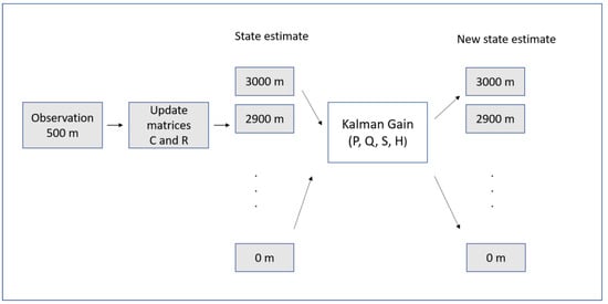
Figure 1.
Diagram block describing the usage of the Kalman filter in AWEA (adapted from de Jong et al., 2014 [12]).
The model was tested near the Schipol airport (the Netherlands) using radar data provided by the Royal Netherlands Meteorological Institute. Two case studies were considered: the first one was an offline simulation, and the second was a fast-time simulation study into aircraft spacing. In the first case, a logarithmic wind profile calculated with a measure from an aircraft (from 0 to 3000 m) with the superposition of a normal distributed noise was used as input for AWEA. The authors used a bootstrap sample extracted from the simulation to calculate the mean and 95% confidence interval of the RMSE (Root Mean Square Error), using ten noise realizations. The numerical simulations revealed that the algorithm is able to reduce the measurement noise from 1.94 knots to 1.35 knots. Moreover, the estimated wind profile can be used to forecast the wind in locations that are positioned farther along the trajectory. The effects of the observation distance were investigated by varying the value of the parameter Kw from 0.1 to 1 in steps of 0.1. The analysis showed that the RMSE value is reduced when Kw is increased, from about 3.5 knots for Kw = 0.1 to 2.2 knots for Kw = 1, confirming the importance of distance information.
In the second case, the ground-based AWEA used broadcast measurements from the aircraft within a TMA to define a single wind profile able to represent the wind field of the entire TMA. Five different implementations of wind estimations were considered, four of them based on AWEA (Table 2).
Table 2.
List of different implementations of wind estimation (adapted from de Jong et al., 2014 [12]).
The RMSE values in estimating the wind along the trajectory are reported in Table 2 for the different scenarios. Results showed that AWEA significantly reduced the RMSE in estimating the prevailing wind. Currently, the availability of meteorological data (including ADS-B) is still limited, but once these reports become widely available, AWEA could be adapted and evaluated in a real-time environment onboard an aircraft.
3. Wind Field Reconstruction with Random Fourier Features
In a recent work, Kiessling et al. [13] analyzed a method for wind field reconstruction based on a machine learning approach and compared it with well-established interpolation techniques. Their approach was mainly devoted to the support of wind farm planning, for which measurements are used to estimate the expected aggregate energy output. The model considered approximates data using a Fourier series, exploring the frequency domain by using a Metropolis [25] adaptive algorithm: at each step, the Fourier coefficients are optimized with respect to a loss function. This method does not consider previous or future time steps, then only a subset of the physical hypothesis on the system is actually applied. The model includes the hypothesis of divergence-free flux, which is always applied in the mesoscale atmospherical models [26]:
where is the velocity vector (m/s). The basic idea of random Fourier features is to define an explicit feature map that is of a dimension lower than the number of observations, but with the resulting inner product which approximates the desired kernel function. The definition of interpolation models was restricted to approximations of specific functions in a two-dimensional range, since only the horizontal wind vector is considered. Specifically, the authors defined a spatial interpolation model as a map f from a set of measurements of velocity to a vector field fd. This process for the definition of a model f is defined as “training” and is performed by minimizing a loss function. There is an important distinction between f and fd, since the function f represents a model that is trained on the original data and produces a vector field fd that approximates the velocity vector . In the classical Fourier series models, the coefficients are defined as:
and the parameters are estimated by optimizing with respect to the expectation of a loss function. In the random Fourier features instead, the optimization is made with respect to the Fourier frequencies ωk. In this view, the random Fourier features are an example of a neural network with a hidden layer and a trigonometric activation function [25]. In particular, ω are the weights connecting the inputs x to the hidden layer, and β are the weights connecting the nodes in the hidden layer to the output layer. In other words, it is the training algorithms that distinguish the random Fourier features.
In order to perform benchmark activities, the following classic algorithms were considered as references: nearest neighbors, inverse distance weighting (IDW), kriging [27], random forest, and neural network. The quality of the reconstruction with the model considered with respect to the classical models was measured using the Q(f) indicator, defined as the mean square deviation of the data provided by the model f(x) against observational data u.
The indicator ε(f), obtained by normalizing Q(f) with respect to the expected squared velocity, was used too. The analysis of the results showed that the random model Fourier features provide the best results against the other models tested. Table 3 shows the differences in the values of indicators Q and ε related to the random Fourier features and the values related to the other models. These differences clearly show that the present method has better performances, in a statistically significant matter, with respect to other methods. Moreover, the authors indicated that a more advanced model, made up of an average between the random forest and the random Fourier features, is able to further improve the performance.
Table 3.
Differences in the values of ε(f) and Q(f) related to the random Fourier features and the other models (data from Kiessling et al., 2021 [13]).
4. The Meteo Particle Model (MPM)
This model was introduced by Sun et al. [14] with the aim of providing an estimate of atmospherical variables inside the airspace using a Monte Carlo approach, using only surveillance data from aircraft. The original method is applicable to both wind and temperature fields. The main idea is based on the usage of a stochastic process to obtain meteorological information in a short time range (from minutes to one hour) in areas where observations are lacking, starting from data collected along high-density flight trajectories. Wind and temperature states are reconstructed using virtual particles that are generated every time new observations are available (of wind and/or temperature) and that then propagate and decay over time. In this way, particle propagation allows the evaluation of atmospherical variables in those areas where measurements are not available. On the basis of the MPM model, it is possible to build a short-term wind predictor based on a time-dependent statistical model (Gaussian Process Regression, GPR). The GPR predictor can be built for each position of interest, in order to provide short-term forecasts. However, it is necessary to record a short chronology of the states estimated by the MPM model.
The model is composed of three steps, described in the following subsections.
4.1. Selection of Input Data
The ensemble of measurements performed by the different aircraft represents a measurement array [x, y, z, u, v, T] including spatial coordinates, wind components and temperature. Initially, a probabilistic selection process is used to remove wrong measurements that could occur, specifically:
- A Gaussian probabilistic function is built starting from the current field, once that mean μ e variance σ has been calculated:In which k1 is a control parameter defined as the acceptance probability factor.
- New data selection: each new data has a p probability of being accepted, in such a way that data related to extreme values have a low probability of being selected. The numerical value assigned to k1 is defined by the user in an empirical way, and its value can be augmented to allow a larger tolerance (increase in the number of accepted measurements). The value proposed by the authors of the method is 3.
4.2. Construction of Particles
A particle is defined as an object able to provide information on the state of wind and temperature. Particles are generated every time new wind measurements (u, v) are available: in particular, for each measurement, N particles are generated close to the position of the aircraft that performed the evaluation. Each particle is characterized by the age (set equal to zero at the time of initialization and increased at the successive steps) in such a way that, at a fixed age, the oldest particles are removed. A small variance is then assigned at the state carried by each particle, to consider the measurement uncertainties. Successively, it is assumed that particles move according to a Gaussian random walk model, i.e., the coordinates xp, yp, zp (m) of the N particles (xp,i, yp,i, zp,i, with i = 1, … N) at the new time step t + Δt are evaluated on the basis of the positions at the previous step t using the following expressions:
In which the ΔP factor is calculated as
Along the horizontal direction (x and y), particles move according to a random track characterized by a small bias (σ), conveniently controlled by the k2 factor (particle random walk factor). Along the vertical direction (z), the propagation follows a zero-average Gaussian track. All the particles are re-sampled at the end of each step. The time step Δt is chosen according to criteria of numerical stability, considering the time frame of the specific application, e.g., the size of the geographical domain, the time interval between two successive measurements, and the time step of the NWP (if the MPM is coupled with an NWP, see Section 6). The particles that for their motion fall outside the domain (both in horizontal and vertical directions) are removed, while the remaining ones are classified according to their age, according to the following probability function:
where α is a number that represents the age of the particle and σα is a control parameter (aging parameter). This resampling ensures a periodic particle renewal, in such a way that the oldest ones are removed.
4.3. Evaluation of Variables Value in a Generic Point
Numerical values of wind and temperature at each position can be calculated by using information carried by the surrounding particles. In particular, the wind in a generical position is evaluated as a weighted average of the wind values carried by the particles belonging to an ensemble P, which includes all the particles whose coordinates x,y,z are within a maximum predetermined distance from the coordinates of the position being considered.
where the previous sums extended to all the particles of the P ensemble. The weight Wp assigned to each particle is calculated as a product of two exponential functions:
The first function establishes a relationship between the weight itself and the distance d (m) between the particle and the position considered, and the second one establishes a relation between the weight and the distance d0 of the particle from its origin:
in which Cd is a control parameter (weighting parameter). These formulae are based on the IDV technique (Inverse Distance Weighted) [28].
The MPM model does not use a predefined grid, meaning that the numerical values can be calculated in a generical point at the current hour, provided that a sufficient number of particles is present in the neighborhood of the point (generally at least ten). Once wind and temperature values have been reconstructed, it is possible to evaluate the confidence level by using a combination of confidence functions based on different factors, including, for example, the number of particles close to the position of interest, the average distance between the particles and the position of interest, the homogeneity of the values carried by the particles and the “strength” of the particles in relation to their age. The different confidence factors obviously assume values within different ranges; for this reason, it is important to normalize these values at the same range of variability (0, 1), for example, by using a linear scaling technique:
5. Examples of Application of the MPM
5.1. The Metsis Project
The METeo Sensors In the Sky (METSIS) [29] project was realized with the aim of contributing to the wind nowcasting inside the U-SPACE Weather Information Service. The main purpose was the evaluation and communication of local wind data in real time to drone operators. These data are generated starting from data measured by the drones themselves. Specifically, a ground station receives wind data from drones and performs a three-dimensional wind field estimation on the area considered by using the MPM. Data are then provided to the drone operators by using the mentioned information service. Wind fields are updated every time new measurements are received from individual drones. This approach could potentially improve flight efficiency and security, since the wind greatly affects the battery duration. Moreover, it represents a low-cost solution for wind nowcasting that could also be applied to different applications. Some limitations are related to the fact that wind estimation can be produced only if a sufficient number of drones are already flying in the area considered; this limitation could be mitigated by using measurements from ground anemometers too. The approach used is the one originally developed in [14] for wind speed estimation at higher altitudes. The MPM evaluates wind fields by using a Monte-Carlo approach, assuming that these fields are pseudo-static on a short time scale, being also able to consider the effects of the presence of obstacles (trees, buildings). Since the current implementation of MPM is aimed at estimating low-altitude wind (<150 m), it is necessary to also consider the vertical component and the interaction with the soil, which is carried out by resetting the particle altitude at the soil level if it ends up under the ground. Alternatively, it is possible to bounce the particles on the ground with a specular reflection of the wind direction. Measurements are performed by mounting ultrasound anemometers on the drones on the top of a 50 cm aluminum pole, to reduce the effects of turbulence induced by the propeller on the measurement [30].
Sunil et al. [29] evaluated the accuracy of wind estimations provided by the METSIS system using a series of experiments. They used three measurement drones to collect data needed to feed MPM and a reference drone used to determine the accuracy of the methodology. A comparison was made between the output of MPM with the measurements provided by the reference drone. Measurement drones (M) were located in such a way as to form an equilateral triangle (Figure 2), while the reference drone flies among four predefined positions. Several triangle sizes were considered, along with two different scenarios (static and dynamic). In the static scenario, the three M drones are located in the three angles, while in the dynamic one, they fly from one angle to another, resulting in a circular trajectory, while R is always static in both scenarios. Three independent variables were considered: type of obstacle (none, trailer, tree), triangle size and altitude, as summarized in Table 4.
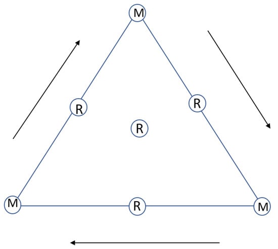
Figure 2.
Position of the reference and measurement drones. Arrows indicate the flight direction of measurement drones (adapted from Sunil et al., 2021 [29]).
Table 4.
List of variables considered in the experiments by Sunil et al., 2021 [29].
The accuracy was measured through the Mean Absolute Error (MAE):
where N is the number of observations, ei represent the MPM estimates and oi are observational values. MAE was evaluated both for wind speed and for the three direction angles, for each scenario considered.
Table 5 shows the MAE of wind speed and three directions for both static and dynamic scenarios, considering the three obstacles. The World Meteorological Organization (WMO) provides standard values for the accuracy of wind measurements, specifically 0.5 m/s (<5 m/s), 10% (>5 m/s) for speed and 5° for directions [31]. These standards can be used as a reference for an initial understanding of the feasibility of METSIS. MAE related to the wind speed results were larger for the scenarios including an obstacle, but its value was not excessively larger than that related to the base condition: even if obstacles have a non-negligible effect on the wind velocity, MPM accuracy is not influenced by them. On the other side, direction accuracy was rather scarce, especially during dynamic tests. In particular, it was found that larger direction errors are related to smaller wind speeds: a part of this bias can be attributed to the inaccuracy of selected anemometers for low wind speeds. Effects of obstacles do not affect the precision if measurements are available close to the obstacles themselves. Further sensitivity tests showed that, as expected, the increase in the measurement drone numbers can be useful to improve the MPM accuracy, since it is a method exclusively based on data and does not make any assumption on the wind dynamics. An analysis aimed to quantify the effects of random measurements on the accuracy was performed by adding two Gaussian noise models to the wind data, respectively, characterized by standard deviation of 0.5 and 1 m/s. The results showed that the two noise models had virtually no effects on the accuracy and that the METSIS concept can be applied on wider scales.
Table 5.
Mean average error (MAE) of wind speed and directions considering the three different obstacles, for (a) static and (b) dynamic scenarios (data extracted from Figure 9 of Sunil et al., 2021 [29]).
5.2. Wind Field Reconstruction at Delft (the Netherlands)
The MPM method was applied by Sun et al. [32] for the reconstruction of wind fields starting from observational data ADS-B [20] (surveillance technique entrusted to aircraft that transmit their position and other information derived from onboard systems, such as GNSS) and Mode-S [33], for an area of about 600 km of diameter, located in the vicinity of Delft. Wind vectors were calculated on a three-dimensional grid starting from data collected continuously (87,600 measurements) in one hour, from 11:30 to 12:30 on 27 July 2017. For every second, the system receives 11 observations from different zones. The results provided by MPM were validated by using data provided by meteorological models as reference, in particular, the analyses of the GFS model [34], for one week. Of course, it must be considered that a part of the error is due to the uncertainty that inevitably affects the reference data provided by GFS, while a part is due to the uncertainty of the data collected onboard. The evaluation was performed in terms of wind direction (considering the angle between the velocity vector calculated by MPM and the one provided by GFS) and in terms of intensity (quantifying the difference of the modules of the mentioned vectors). The analysis was split into two parts, considering moderate winds (less than 10 m/s) and more intense ones (larger than 10 m/s), respectively. The average errors over the considered periods resulted in about 5 m/s and 20° for moderate winds, and about 4 m/s and 10° for intense winds. It is evident that for low wind speeds, results are less aligned with the GFS model data. However, as stated by the authors in [32], this does not imply that results are less accurate, but rather that values provided by GFS are smoothed and interpolated over much larger periods of time and areas. As regards the error distribution, for moderate winds the 25th (Q1) and 75th (Q3) percentiles speed errors are, respectively, equal to 3.5 and 7 m/s, while the whole range of errors is between 2 and 11 m/s; for directions, Q1 and Q3 are 18° and 28°. For more intense winds, Q1 and Q3 are, respectively, equal to 3 and 5 m/s, while the whole range of errors is between 2 and 6 m/s; for directions, Q1 and Q3 are 8° and 12°. In all cases, no outliers are recorded.
For its intrinsic nature, MPM is characterized by a level of randomness, which is essential for some aspects, in order to simulate the uncertain wind behavior. However, it is necessary to verify if this level of randomness does excessively influence the forecast. This verification can be carried out by repeating several times the same simulation and calculating the relevance of the difference in the results. In the test case considered, the simulation was repeated 100 times, recording a maximum difference of 1° for the direction and 1 m/s for the intensity, which can be considered acceptable. Moreover, it is necessary to quantify the model sensitivity to the availability of observational data to be provided as input to the MPM. For this reason, the MPM simulation was repeated by gradually reducing (in a random way) the quantity of input data, precisely at 90%, 70%, 50%, 30% and 10% of the total amount of data available. This kind of analysis shows that with up to 50% data loss, the accuracy still remains at an acceptable level. This test demonstrates that, within a reasonable percentage of data uncertainty, the MPM is able to provide relatively stable wind field results.
Finally, it is evident that a factor that significantly influences the correctness of the results is the input data accuracy. In order to quantify this effect, an assigned percentage (p) of input data (respectively p = 2%, 4%, 6%, 8%, 10% and 15%) was replaced by uniformly distributed random values. The analysis showed that, as expected, the average error values of the MPM output grow with p, but they remain behind reasonable limits when p is less or equal to 6%.
5.3. Model Extension at Different Heights
The applicability of the MPM method to different levels of altitude was investigated by Zhu et al. [35]. The area object of study was the same already considered in [32], i.e., an area of about 600 km of diameter located in the vicinity of Delft. As input, the authors used data provided by the ADS-B system. The accuracy of the forecasts obtained with MPM was verified assuming the ERA-5 reanalysis [36] at resolution 0.25° as reference.
ERA-5 is the fifth generation of ECMWF reanalysis for the global climate and weather for the past eight decades. The evaluation was performed on 1 January 2018 at hours 0, 6, 12 and 18 UTC, using the classic indices MAE, RMSE, COR (Pearson Correlation Coefficient) and R (cosine similarity coefficient), applied to the wind velocity vectors. Moreover, an index that combines COR and R was defined, which is particularly suitable for vector comparisons, such as wind velocity:
in which α is a numerical coefficient chosen in an empirical way, which in the present study was set equal to 0.5.
Figure 3 shows (a) the retrieval of the wind field from 17:59:10 to 18:00:50 and (b) the instantaneous wind provided by ERA-5 reanalysis at 18:00:00 as the reference data. A comparison of the two maps shows that the wind field distribution is basically the same.
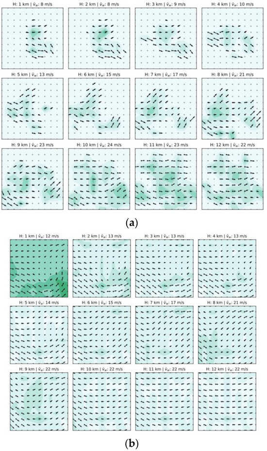
Figure 3.
(a) Retrieval map of wind field during 17:59:10~18:00:50. (b) Wind field map of ECMWF ERA-5 data at 18:00:00 (from Zhu et al., 2021 [35]).
Model performances were analyzed in different periods, at various altitudes. It can be seen that the wind values range between 12 m/s at 1 km of altitude and 22 m/s at 12 km of altitude; the MAE speed error grows with the altitude (from 1 m/s at 1 km to 8 m/s at 12 km), while MAE related to the direction is in the range between 4 and 14°, with wind speed precision generally better than the direction one. The main factor affecting the quality of results is the amount of input data available; in particular, it was clear that the model requires a fixed minimum amount of data to properly work. In order to improve the MPM performances, the authors modified the values of some empirical constants and control factors used by the method (defined in Section 4), as shown in Table 6.
Table 6.
Original and optimized values of some control factors defined in MPM (data from Zhu et al., 2021 [35]).
The application of these new values allowed a performance improvement, as it is possible to verify by comparing the original monitoring indices values with those obtained with the application of the optimized factors (Table 7).
Table 7.
Original and optimized values of some control factors defined in MPM (data from Zhu et al., 2021 [35]).
Of course, it must be considered that ERA-5 are usually smooth data and generally do not have local changes, so it is possible that a part of the errors recorded is due to the reference dataset, which to some extent neutralizes the advantages of the algorithm.
6. NWP Models
As explained in the previous sections, limitations in the applications of wind field reconstruction methods are related to the fact that estimations can be produced only if a sufficient number of drones is already flying in the area considered; this limitation could be mitigated using measurements from ground anemometers or using data provided by Numerical Weather Prediction models (NWPs). Scientific and technological developments have led to increasing the weather forecast capabilities over the past 40 years. In ref. [37], Mazzarella et al. investigated if NWP-based short-range high-resolution weather forecasts (including data assimilation) can improve the predictive capability of extreme events, to understand if such forecasts can be suitable to support air traffic management. NWPs take current weather observations as input through process-defined data assimilation aimed to produce initial conditions for the meteorological variables (from the oceans to the top of the atmosphere). The derivation of the current state (the analysis) of the atmosphere is treated as a Bayesian inversion problem using observations (even from drones), previous information from forecasts and related uncertainties as constraints. These calculations involve a global minimization and are performed in four dimensions to produce an analysis that is physically consistent in space and time and can deal with observational data that are heterogeneously distributed in space and time, such as those provided by drones themselves. NWPs deliver weather forecasts by solving the full set of prognostic equations upon which the evolution in the atmosphere of wind, pressure, density and temperature is described [9]. These equations are solved numerically using temporal and spatial discretization, and this technique provides a distinction between resolved and unresolved scales of motion. Physical processes on unresolved scales need to be parameterized in terms of their interaction with the resolved scales. NWPs are classified into two categories: General Circulation Models (GCMs) and Limited Area Models (LAMs). GCMs perform simulations considering the global atmosphere and are characterized by a low resolution. Limited Area Models are used to obtain detailed information over a specific area of interest and they allow the usage of a higher resolution. GCMs are important also because they provide initial and boundary conditions to LAMs; in the present study, the attention is focused only on LAMs because they are widely used to support civil aviation. Several LAMs are available and are currently operationally used by national meteorological forecast services. Among them, the Weather Research and Forecasting (WRF) Model [15] is the most popular mesoscale weather prediction system designed for both atmospheric research and operational forecasting applications. It features two dynamical cores, a data assimilation system, and a software architecture supporting parallel computation and system extensibility. The COSMO model [5] was developed by the European consortium COSMO (Consortium for Small-scale Modeling). COSMO is a non-hydrostatic limited area model for three-dimensional compressible flows, based on the primitive hydro-thermodynamical equations. The model equations are solved numerically on a rotated latitude–longitude grid, with terrain-following coordinates in the vertical, using a Eulerian finite difference approach. In 2018, the COSMO consortium started the migration from the COSMO-LM to the ICON-LAM (ICON Limited Area Model) [6] as the future operational model. It employs an unstructured grid made up of regular icosahedra and the spatial discretization is performed using an icosahedral–triangular C grid. The vertical coordinate system is height based and follows the terrain, so the top and bottom triangle faces are inclined with respect to the tangent plane on a sphere.
Currently, thanks to the growth of computational resources, LAMs can be run at a spatial resolution of about 1 km, which is not sufficient to support drone operations in urban contexts. For this reason, further enhancements are still needed, as discussed in the next section.
7. Discussion and Conclusions
Current research shows that the treatment of the retrieved wind field is still incomplete and a big effort from the scientific community is needed to cope with the chaotic nature of wind, the movement of aircraft, and the non-uniform distributed network of observations. In the framework of the EDUS project, CIRA is defining an operating platform demonstrator based on the existing CIRA Meteo Service Center in order to integrate data and algorithms with newer ones, aimed at treating the urban wind, in particular the evaluation of the three components from soil up to 3 km of altitudes. A promising approach could be based on the integration of monitoring “low cost and mobile” data and other sources, such as those available from the COPERNICUS program (copernicus.eu), especially for what concerns urban areas. Given the current lack of meteorological data available in urban environments, the usage of existing measurement networks will be increased, such as those coming from universities, regional agencies, civil protection and small airports. Of course, the installation of new sensors will be required, according to local stakeholders. These stations will represent the “ground truth” of remote sensing data and, along with all the data sources available, will allow the monitoring and nowcasting at high resolution of wind and other variables.
In the present work, the main methodologies used to reconstruct wind fields at low altitudes in urban areas have been analyzed:
- AWEA estimates wind profiles using measurements of wind data taken from nearby aircraft, providing high-fidelity and high-resolution user-tailored wind profiles, which can be used for predicting wind at locations farther along the trajectory with small errors. The power law equation used in AWEA only yields a very general approximation of the wind profile in the PBL. Especially since the PBL is characterized by the interaction between the free stream wind at higher altitudes and the disturbing forces of friction caused by the Earth’s roughness, this approximation can differ from the true wind profile. However, in order to derive a useful model not dependent on local surface roughness or latitude, this power law is used as a first approximation of the wind profile and could also be used to fill the gaps when measurement data is sparse. For this reason, the dependence on the surface roughness length was neglected. In future developments, the usage of historical data and cross-correlations between time series provided by different aircraft would improve the accuracy of the results.
- The random Fourier features is a novel interpolation model that results competitively with respect to other statistical interpolation models, such as kriging or modern machine learning methods, e.g., random forests and neural networks. The authors found that the model can be extended to new areas of research, including, for example, the possibility of incorporating data over multiple times and including more terrain-specific features. Since the definition of interpolation models was restricted to a two-dimensional range (only the horizontal wind vector is considered), better accuracy would be provided by the introduction of a modified coordinate system, defined to follow the terrain.
- The MPM concept demonstrated the possibility of using drones as a large sensor network to construct a global scale real-time meteorological measurement system. However, the accuracy for wind direction did not meet the WMO standards [31]. On the other side, the effects of obstacles on wind can be considered without affecting performances, as long as wind measurements are available near the obstacles. The near-surface turbulence is a source of difficulty in wind field reconstruction. For example, Kiessling et al. [13] found non-negligible interpolation errors related to this kind of turbulence; in particular, they found that the error is lower during nighttime: in the summer period this can be explained by the observed reduction in wind speed during night time; instead, in winter, even if wind speeds are higher, the atmosphere tends to be more stable at nighttime [38], which might explain this decrease in error.
Currently, the methods described in this work are not able to consider the influence of this part of turbulence. In particular, the MPM model assumes that the true state of wind and temperature is geographically stable at the level of tens of kilometers. This hypothesis ensures that the atmospheric state at any location can be represented by observations made in adjacent areas. However, it is well known that turbulence breaks this assumption, and so it cannot be represented accurately by this model. Recent studies, e.g., ref. [39], proved that fine-resolution NWP have good capabilities in predicting the phenomenon of low-level turbulence and wind shear for aviation weather applications. For this reason, in the opinion of the author, a step forward could be represented by the coupling of NWP models with the MPM, for the feasibility features and accuracy in the results obtained with this model; in fact, the MPM addresses the stochastic characteristic of wind through particles and maintains the stability through the use of a sufficiently large number of particles. Moreover, compared to Gaussian weighted interpolation, the MPM maintains past observation information without the need for large historical measurement storage [14]. The coupling with an NWP will ensure that estimations can be produced in any geographical area, not only where a sufficient number of drones are already flying. It could be realized in such a way that the MPM reads the hourly NWP output at high resolution (about 1 km), generates particles at each grid point and provides wind values at minute frequency in a generical point considered for the investigation. The first results related to the coupling of MPM with the NWP COSMO over an area located in southern Italy [40] will be presented in future work.
Funding
This research was carried out in the frame of the CIRA internal project PRORA 662 SES-AAM EDUS, funded by the DM 662/2020 of the Italian Ministry of Education.
Data Availability Statement
No new data were created or analyzed in this study. Data sharing is not applicable to this article.
Acknowledgments
Vittorio Di Vito (CIRA) and Giulia Torrano (CIRA) are gratefully acknowledged for the effective management of the EDUS project.
Conflicts of Interest
The authors declare no conflict of interest. The funders had no role in the design of the study; in the collection, analyses, or interpretation of data; in the writing of the manuscript; or in the decision to publish the results.
References
- Barrado, C.; Boyero, M.; Brucculeri, L.; Ferrara, G.; Hately, A.; Hullah, P.; Martin-Marrero, D.; Pastor, E.; Rushton, A.P.; Volkert, A. U-Space Concept of Operations: A Key Enabler for Opening Airspace to Emerging Low-Altitude Operations. Aerospace 2020, 7, 24. [Google Scholar] [CrossRef]
- SESAR Joint Undertaking. European ATM Master Plan: Roadmap for the Safe Integration of Drones into all Classes of Airspace. Tech. Rep. Mar. 2017. Available online: https://www.sesarju.eu/node/2993 (accessed on 6 October 2023).
- Fang, Z.; Zhao, Z.; Du, L.; Zhang, J.; Pang, C.; Geng, D. A new portable micro weather station. In Proceedings of the 2010 5th IEEE International Conference on Nano/Micro Engineered and Molecular Systems, Xiamen, China, 20–23 January 2010; pp. 379–382. [Google Scholar] [CrossRef]
- Rillo, V.; Zollo, A.L.; Mercogliano, P. MATISSE: An ArcGIS tool for monitoring and nowcasting meteorological hazards. Adv. Sci. Res. 2015, 12, 163–169. [Google Scholar] [CrossRef][Green Version]
- Steppeler, J.; Doms, G.; Bitzer, H.W.; Gassmann, A.; Damrath, U.; Gregoric, G. Meso-gamma scale forecasts using the nonhydrostatic model LM. Meteorol. Atmos. Phys. 2003, 82, 75–96. [Google Scholar] [CrossRef]
- Zängl, G.; Reinert, D.; Rípodas, P.; Baldauf, M. The ICON (ICOsahedral Non-hydrostatic) modelling framework of DWD and MPI-M: Description of the non-hydrostatic dynamical core. Q. J. R. Meteorol. Soc. 2015, 141, 563–579. [Google Scholar] [CrossRef]
- Klooster, J.; Wichman, K.; Bleeker, O. 4D Trajectory and Time-of-Arrival Control to Enable Continuous Descent Arrivals. In Proceedings of the AIAA Guidance, Navigation and Control Conference and Exhibit, Guidance, Navigation, and Control and Co-located Conferences, Honolulu, Hawaii, 19 August 2002. [Google Scholar]
- Dalmau, R.; Prats, X.; Baxley, B. Using wind observations from nearby aircraft to update the optimal descent trajectory in real-time. In Proceedings of the 2019 13th USA/Europe Air Traffic Management Research and Development Seminar, Vienna, Austria, 17–21 June 2019. [Google Scholar]
- Bauer, P.; Thorpe, A.; Brunet, G. The quiet revolution of numerical weather prediction. Nature 2015, 525, 47–55. [Google Scholar] [CrossRef]
- de Grado, J.G.; Tascon, C.S. On the Development of a Digital Meteorological Model for Simulating Future Air Traffic Management Automation. In Proceedings of the 2011 20th IEEE International Workshops on Enabling Technologies: Infrastructure for Collaborative Enterprises, Paris, France, 27–29 June 2011; pp. 223–228. [Google Scholar] [CrossRef]
- Di Leoni, P.C.; Mazzino, A.; Biferale, L. Synchronization to Big Data: Nudging the Navier-Stokes Equations for Data Assimilation of Turbulent Flows. Phys. Rev. X 2020, 10, 011023. [Google Scholar] [CrossRef]
- De Jong, P.M.A.; Van der Laan, J.J.; In‘t Veld, A.C.; Van Paassen, M.M.; Mulder, M. Wind-Profile Estimation Using Airborne Sensors. J. Aircr. 2014, 51, 1852–1863. [Google Scholar] [CrossRef]
- Kiessling, J.; Ström, E.; Tempone, R. Wind field reconstruction with adaptive random Fourier features. Proc. R. Soc. A 2021, 477, 20210236. [Google Scholar] [CrossRef]
- Sun, J.; Vû, H.; Ellerbroek, J.; Hoekstra, J.M. Weather field reconstruction using aircraft surveillance data and a novel meteo-particle model. PLoS ONE 2018, 13, e0205029. [Google Scholar] [CrossRef]
- Skamarock, W.C.; Klemp, J.B.; Dudhia, J.; Gill, D.O.; Barker, D.M.; Wang, W.; Powers, J.G. A Description of the Advanced Research WRF, Version 3; NCAR Technical note-475+ STR; National Center for Atmospheric Research: Boulder, CO, USA, 2008. [Google Scholar]
- Mondoloni, S. A Multiple-Scale Model of Wind-Prediction Uncertainty and Application to Trajectory Prediction. In Proceedings of the 6th AIAA Aviation Technology, Integration and Operations Conference (ATIO), Wichita, KS, USA, 25–27 September 2006; pp. 1–6. [Google Scholar] [CrossRef]
- Kalman, R.E. A New Approach to Linear Filtering and Prediction Problems, Transaction of the ASME. J. Basic Eng. 1960, 82, 35–45. [Google Scholar] [CrossRef]
- Bienert, N.; Fricke, H. Real-time Wind Uplinks for Prediction of the Arrival Time and Optimization of the Descent Profile. In Proceedings of the 3rd ENRI International Workshop on ATM/CNS, Tokyo, Japan, 19–22 February 2013; pp. 1–6. [Google Scholar]
- De Prins, J.L.; Schippers, K.F.M.; Mulder, M.; Van Paassen, M.M.; In’t Veld, A.C.; Clarke, J.-P.B. Enhanced Self-Spacing Algorithm for Three-Degree Decelerating Approaches. J. Guid. Control. Dyn. 2007, 30, 576–590. [Google Scholar] [CrossRef]
- de Leege, A.M.P.; van Paassen, M.M.; Mulder, M. Using automatic dependent surveillance-broadcast for meteorological monitoring. J. Aircr. 2012, 50, 249–261. [Google Scholar] [CrossRef]
- Delahaye, D.; Puechmorel, S.; Vacher, P. Windfield estimation by radar track Kalman filtering and vector spline extrapolation. In Proceedings of the 22nd Digital Avionics Systems Conference, Indianapolis, IN, USA, 12–16 October 2003; DASC’03. Volume 1, p. 5-E. [Google Scholar] [CrossRef]
- Elfring, J.; Torta, E.; van de Molengraft, R. Particle Filters: A Hands-On Tutorial. Sensors 2021, 21, 438. [Google Scholar] [CrossRef]
- in’t Veld, A.C.; de Jong, P.M.A.; van Paassen, M.M.; Mulder, M. Real-time Wind Profile Estimation using Airborne Sensors. In Proceedings of the AIAA Guidance, Navigation, and Control Conference, Portland, OR, USA, 8–11 August 2011. [Google Scholar]
- Zoumakis, N.M.; Kelessis, A.G. Methodology for Bulk Approximation of the Wind Profile Power-Law Exponent under Stable Stratification. Bound. Layer Meteorol. 1990, 55, 199–203. [Google Scholar] [CrossRef]
- Kammonen, A.; Kiessling, J.; Plecháč, P.; Sandberg, M.; Szepessy, A. Adaptive random Fourier features with metropolis sampling. Found. Data Sci. 2020, 2, 309. [Google Scholar] [CrossRef]
- Pielke, R. Mesoscale atmospheric modeling. In Encyclopedia of Physical Science and Technology, 3rd ed.; Meyers, R.A., Ed.; Academic Press: New York, NY, USA, 2003; pp. 383–389. [Google Scholar]
- Dalmau, R.; Pérez-Batlle, M.; Prats, X. Estimation and prediction of weather variables from surveillance data using spatio-temporal Kriging. In Proceedings of the 2017 IEEE/AIAA 36th Digital Avionics Systems Conference (DASC), St. Petersburg, FL, USA, 17–21 September 2017; IEEE: Piscataway, NJ, USA, 2007; pp. 1–8. [Google Scholar]
- Zhou, J.; Wu, Y.; Yan, G. General formula for estimation of monthly average daily global solar radiation in China. Energy Convers. Manag. 2005, 46, 257–268. [Google Scholar]
- Sunil, E.; Koerse, R.; Brinkman, T.; Sun, J. METSIS: Hyperlocal Wind Nowcasting for U-Space, 11th SESAR Innovation Days. 2021. Available online: https://www.sesarju.eu/sites/default/files/documents/sid/2021/papers/SIDs_2021_paper_88.pdf (accessed on 8 August 2023).
- Sasaki, K.; Inoue, M.; Shimura, T.; Iguchi, M. In Situ, Rotor-Based Drone Measurement of Wind Vector and Aerosol Concentration in Volcanic Areas. Atmosphere 2021, 12, 376. [Google Scholar] [CrossRef]
- World Meteorological Organization. Part I. Measurement of Meteorological Variables—Chapter 5: Measurement of Surface Wind. Tech. Rep. 2014. Available online: https://library.wmo.int/docnum.php?explnumid=3177 (accessed on 6 October 2023).
- Sun, J.; Vu, H.; Ellerbroek, J.; Hoekstra, J. Ground-Based Wind Field Construction from Mode-S and ADS-B Data with a Novel Gas Particle Model, 7th SESAR Innovation Days. 2017. Available online: https://www.sesarju.eu/sites/default/files/documents/sid/2017/SIDs_2017_paper_16.pdf (accessed on 8 August 2023).
- de Haan, S. High-resolution wind and temperature observations from aircraft tracked by Mode-S air traffic control radar. J. Geophys. Res. Atmos. 2011, 116, D10. [Google Scholar] [CrossRef]
- Kanamitsu, M. Description of the nmc global data assimilation and forecast system. Weather. Forecast. 1989, 4, 335–342. [Google Scholar] [CrossRef]
- Zhu, J.; Wang, H.; Li, J.; Xu, Z. Research and Optimization of Meteo-Particle Model for Wind Retrieval. Atmosphere 2021, 12, 1114. [Google Scholar] [CrossRef]
- Hersbach, H.; Bell, B.; Berrisford, P.; Hirahara, S.; Horányi, A.; Muñoz-Sabater, J.; Nicolas, J.; Peubey, C.; Radu, R.; Schepers, D.; et al. The ERA5 global reanalysis. Quart. J. Royal Met. Soc. 2020, 146, 1999–2049. [Google Scholar] [CrossRef]
- Mazzarella, V.; Milelli, M.; Lagasio, M.; Federico, S.; Torcasio, R.C.; Biondi, R.; Realini, E.; Llasat, M.C.; Rigo, T.; Esbrí, L.; et al. Is an NWP-Based Nowcasting System Suitable for Aviation Operations? Remote. Sens. 2022, 14, 4440. [Google Scholar] [CrossRef]
- Achberger, C.; Chen, D.; Alexandersson, H. The surface winds of Sweden during 1999–2000. Int. J. Climatol. 2006, 26, 159–178. [Google Scholar] [CrossRef]
- Hon, K. Predicting Low-Level Wind Shear Using 200-m-Resolution NWP at the Hong Kong International Airport. J. Appl. Meteorol. Climatol. 2019, 59, 193–206. [Google Scholar] [CrossRef]
- Bucchignani, E.; Mercogliano, P. Performance evaluation of high-resolution simulations with COSMO over South Italy. Atmosphere 2021, 12, 45. [Google Scholar] [CrossRef]
Disclaimer/Publisher’s Note: The statements, opinions and data contained in all publications are solely those of the individual author(s) and contributor(s) and not of MDPI and/or the editor(s). MDPI and/or the editor(s) disclaim responsibility for any injury to people or property resulting from any ideas, methods, instructions or products referred to in the content. |
© 2023 by the author. Licensee MDPI, Basel, Switzerland. This article is an open access article distributed under the terms and conditions of the Creative Commons Attribution (CC BY) license (https://creativecommons.org/licenses/by/4.0/).