Comparing the Effects of Wildfire and Hazard Reduction Burning Area on Air Quality in Sydney

Abstract

Landscape fires emit smoke that contains particulate matter (PM) that can be harmful to human health. Prescribed fires or hazard reduction burns (HRBs) and wildfires can substantially reduce air quality in populated areas. While HRBs reduce the size and PM output of future wildfires, they also produce PM. There is a critical question of whether conducting HRBs adds to or reduces the total PM (prescribed + wildfire PM) exposure of populations, which has important community health implications. We modelled mean 24 h PM_2.5 in Sydney from fire type, 24 h active regional fire area and weather predictors. We compared HRB and wildfire area effects via an interaction between fire area and fire type, and we found that a non-linear effect of fire area was most appropriate. We conducted a trade-off analysis by using the model to predict increased HRB area scenarios and calculated the number of HRB and wildfire days with ‘Fair’ or worse air quality under each scenario. Regional HRBs and wildfire areas had similar effects on PM_2.5 in Sydney. Increasing regional HRB area produced substantial increases in HRB exceedance days (>12.5 µgm⁻³) in Sydney but only a small reduction in wildfire exceedance days. Our results indicate that small fires in the region have a higher per-hectare impact on PM levels in Sydney, and consequently, increasing regional HRB area would result in more poor air quality days overall (HRB + wildfire days) in Sydney.

1. Introduction

Landscape fires can be broadly classed as either prescribed fires or wildfires. Wildfires have unplanned ignitions and uncontrolled spread and can result in high fire intensities, the destruction of structures and fatalities. Prescribed fires are ignited by land managers under conditions that allow for containment of fire spread and moderation of fire intensity. Prescribed fires commonly aim to reduce fuels (i.e., hazard reduction burns (HRBs)) or may aim to promote ecological health, including triggering the growth of fire-dependent species [1]. For HRBs, the intention of reducing fuel levels is to limit the intensity, rate of spread and area burnt by future wildfires, making control by crews more likely and protecting people and buildings from wildfire [2]. However, while the benefits of HRBs are documented, there are potentially negative side-effects of HRBs that have not been fully explored. In particular, it is not clear whether strategies for conducting HRBs to reduce future wildfires add to or reduce total landscape fire smoke impacts (wildfire + HRB).

The relative costs of HRBs and wildfires can be captured using various metrics, including firefighting resource and crew costs, fire severity (vegetation damage) and damage to buildings and assets. HRBs are conducted in a controlled manner, so in most cases, fire severity is limited, and damage to buildings and assets is unlikely, mainly occurring on rare occasions where the fire escapes control lines [3]. However, both HRBs and wildfires always produce smoke that can cover large areas and contain pollutants that are damaging and costly in terms of human health [4,5]. Particulate matter < 2.5 µm in diameter (PM_2.5) is a routinely measured pollutant because these particulates can be inhaled and can lead to health issues amongst exposed populations that include airway inflammation, asthma attacks and increases in cardiovascular diseases. Effects of PM_2.5 can be apparent at regional scales through increased hospitalisations and premature deaths [5,6].

There is a benefit–cost trade-off between wildfire smoke and HRB smoke, which Jones et al. [7] describe as more smoke today (from prescribed fires; ‘a cost’) for less smoke tomorrow (from wildfire; ‘a benefit’) and which is also detailed in Williamson et al. [8]. The cost of increasing HRB smoke (thus PM) output by conducting more HRBs should have the benefit of less wildfire smoke because HRBs reduce the size of future wildfires. Ideally, this would result in fewer total (wildfire + HRB) smoke impacts. However, this trade-off question has not been fully explored in research despite increases in area burnt via HRBs in recent years [7]. The question is complicated by the fact that HRBs and wildfires may have different per-hectare effects. For the metric of fire area, there is not a one-to-one reduction in wildfire area due to HRB area: on average, around three hectares of HRBs are needed to reduce wildfire area by one hectare (i.e., ‘leverage’) [9,10]. For smoke and pollutant output, further research is needed, but per-hectare differences between HRBs and wildfires could result from differences in fire characteristics and behaviour: wildfires can be more intense and consume more canopy and tree fuels than HRBs [11]—high-intensity wildfire runs produce plumes that can extend high into the air which can mean less smoke at the surface depending on plume depth [12,13]; smoke from a nearby HRB has a greater effect than distant wildfire smoke and HRBs tend to be ignited nearer communities, where they are applied to maximise risk reduction to adjacent property [14,15]. Many factors and interactions are at play that make analysis of this trade-off a challenging task. Nevertheless, a deeper understanding of the trade-off between wildfire and HRB smoke is required to inform fire management practices to achieve the best possible health outcomes for communities.

Few studies have compared wildfire and HRB smoke and its effects on air quality. Borchers-Arriagada et al. [16] calculated and compared health costs associated with days described as either wildfire- or HRB-dominated and found that HRB days had between 1.2 and 4.6 times the per hectare cost of wildfires (although wildfires had greater total cost over their study period). However, the finding of a 4.6 times cost was driven by large outlier wildfire years and removing those resulted in only 1.2 times the cost. Given the lack of research and variation in existing research, there is a low level of confidence in our current understanding here. Additional separate analyses are needed to add evidence to achieve a better understanding and provide clearer directions for fire managers.

Here, we analyse the differences between HRB and wildfire-associated PM_2.5 levels in Sydney, Australia, which is subject to regular wildfires and HRB programs in surrounding areas of native vegetation. The main questions were:

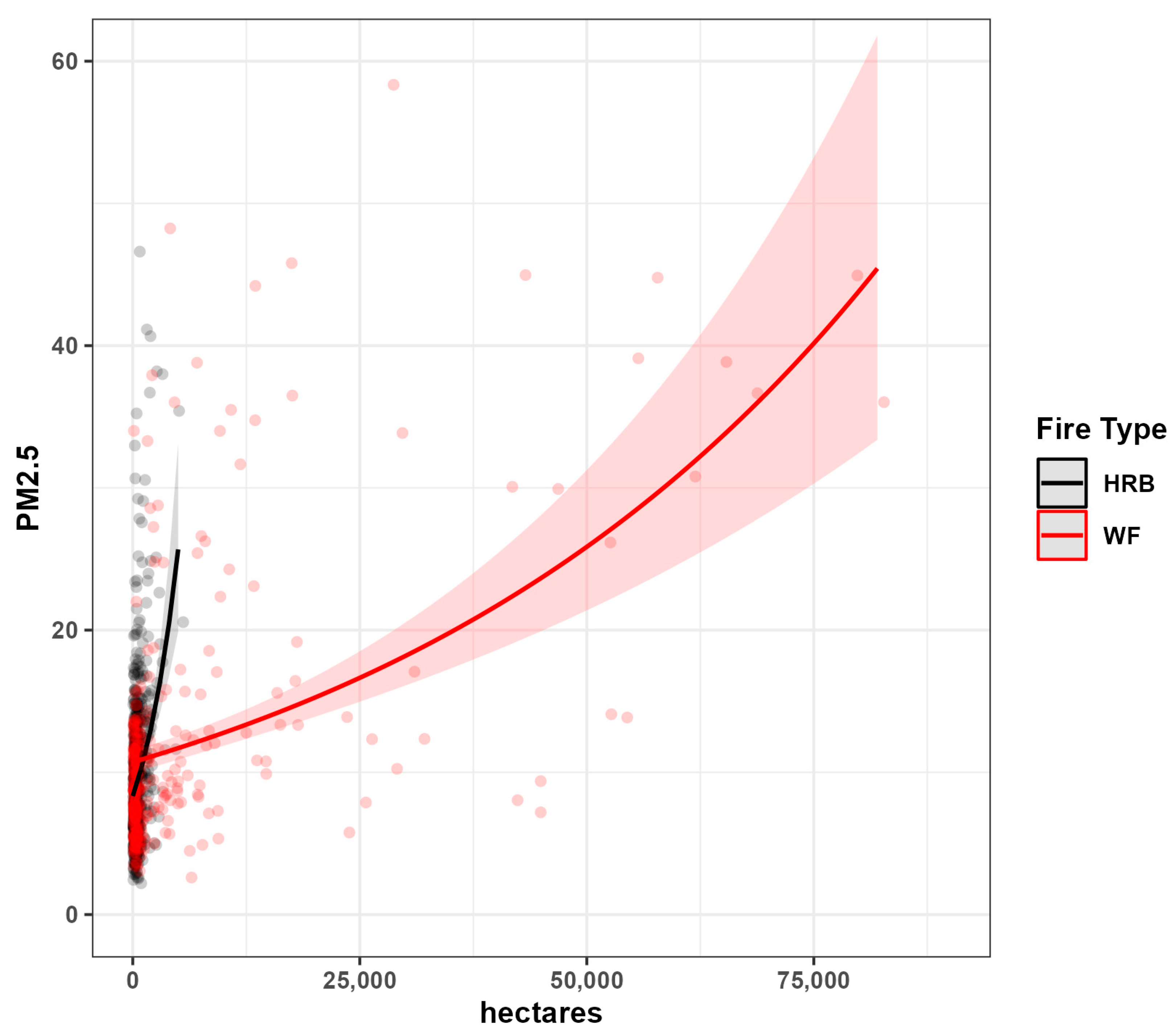
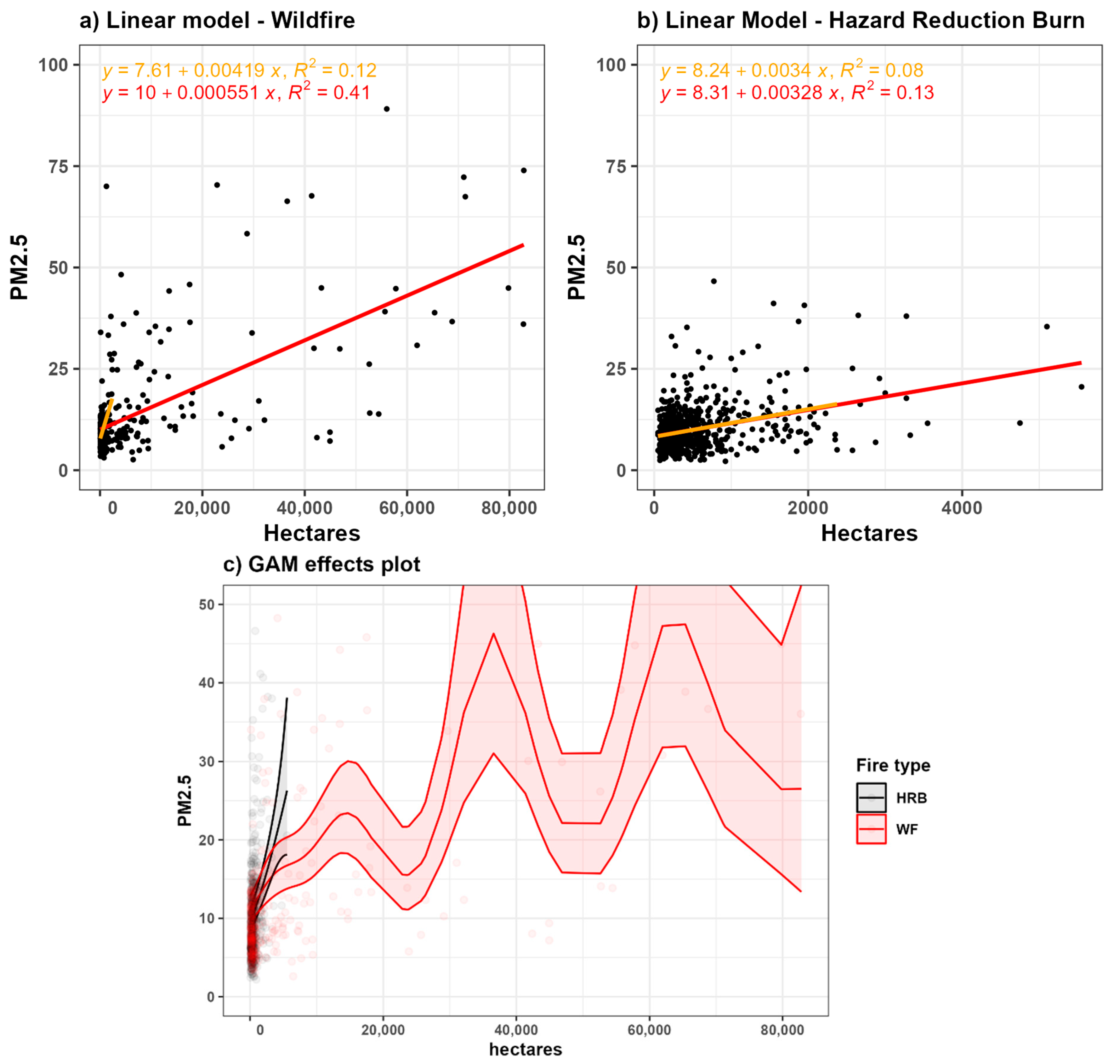
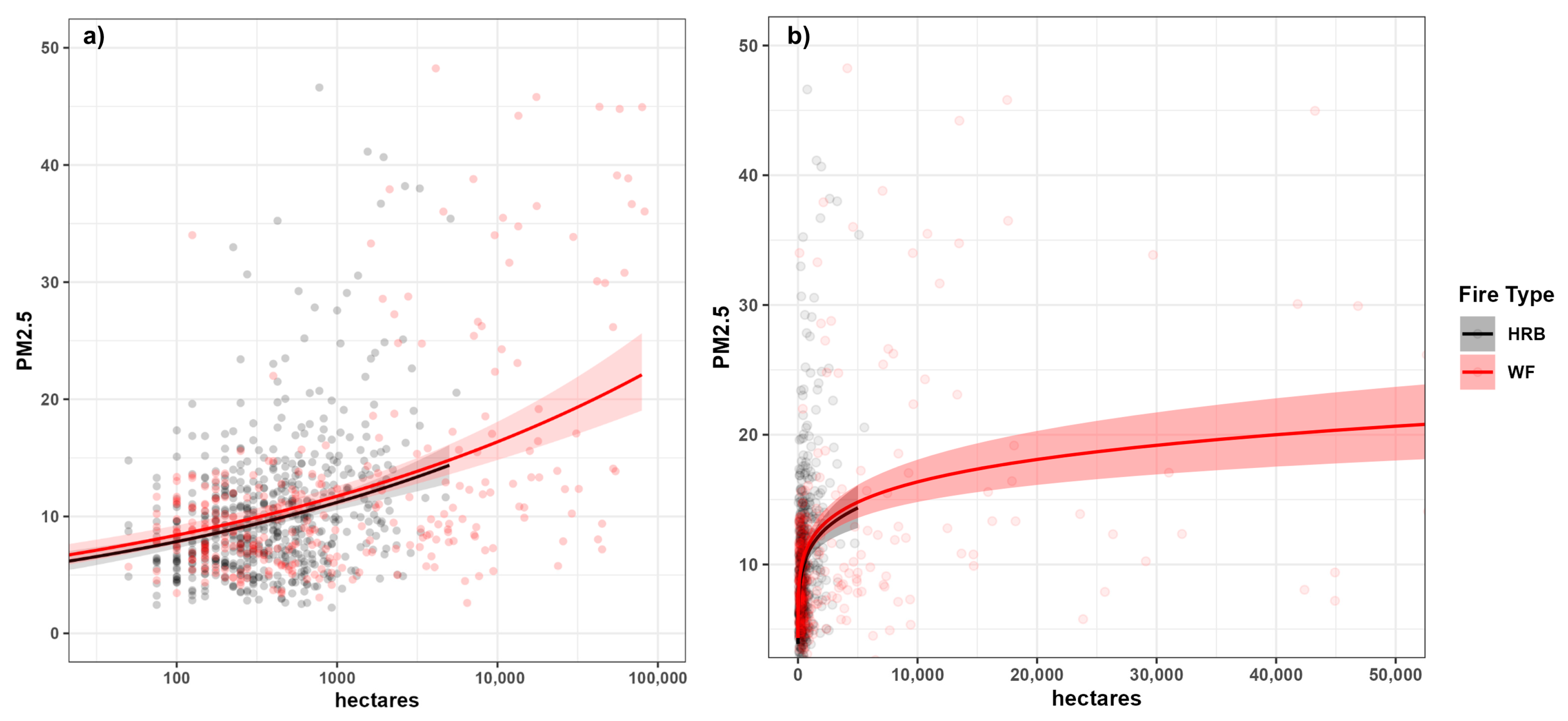
• Is there a difference between the effect of HRB area and wildfire area on air pollution in Sydney, as measured by 24 h mean PM_2.5?
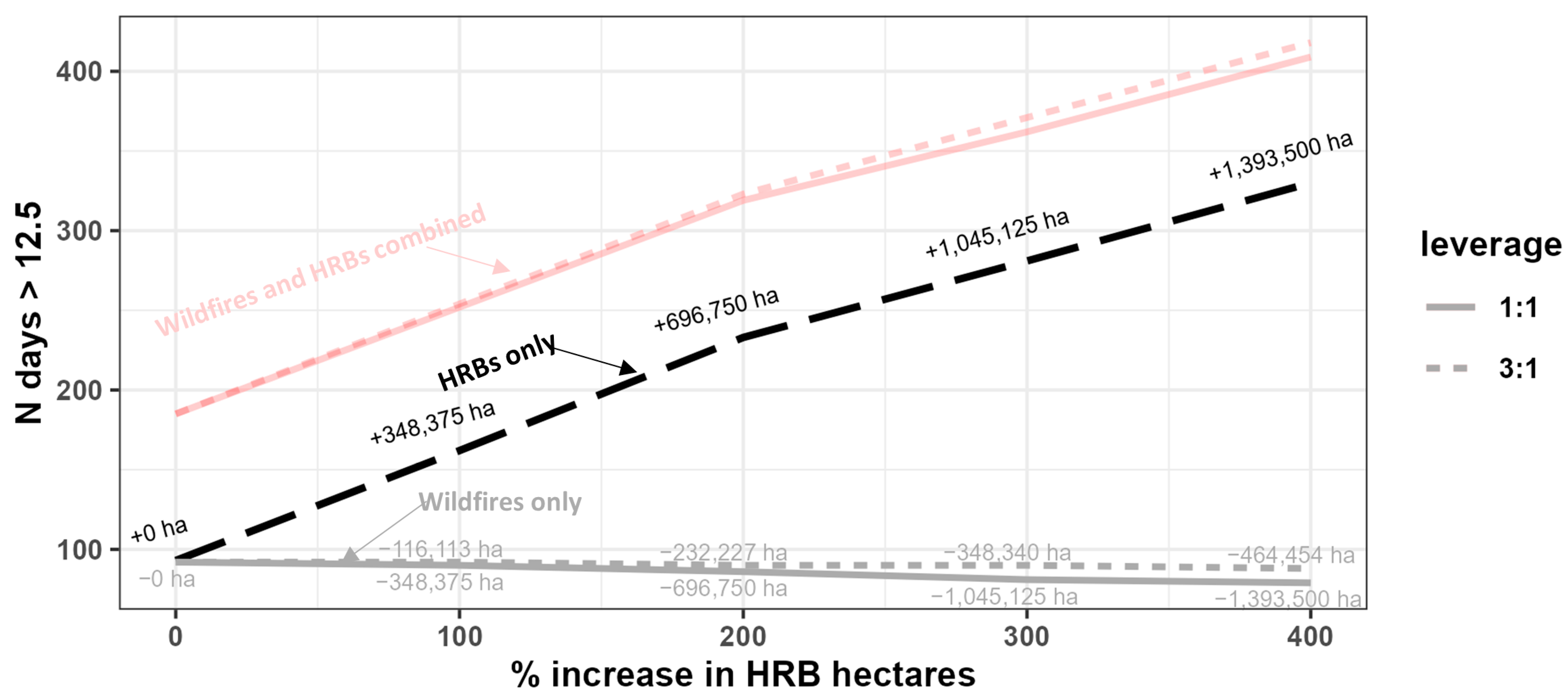
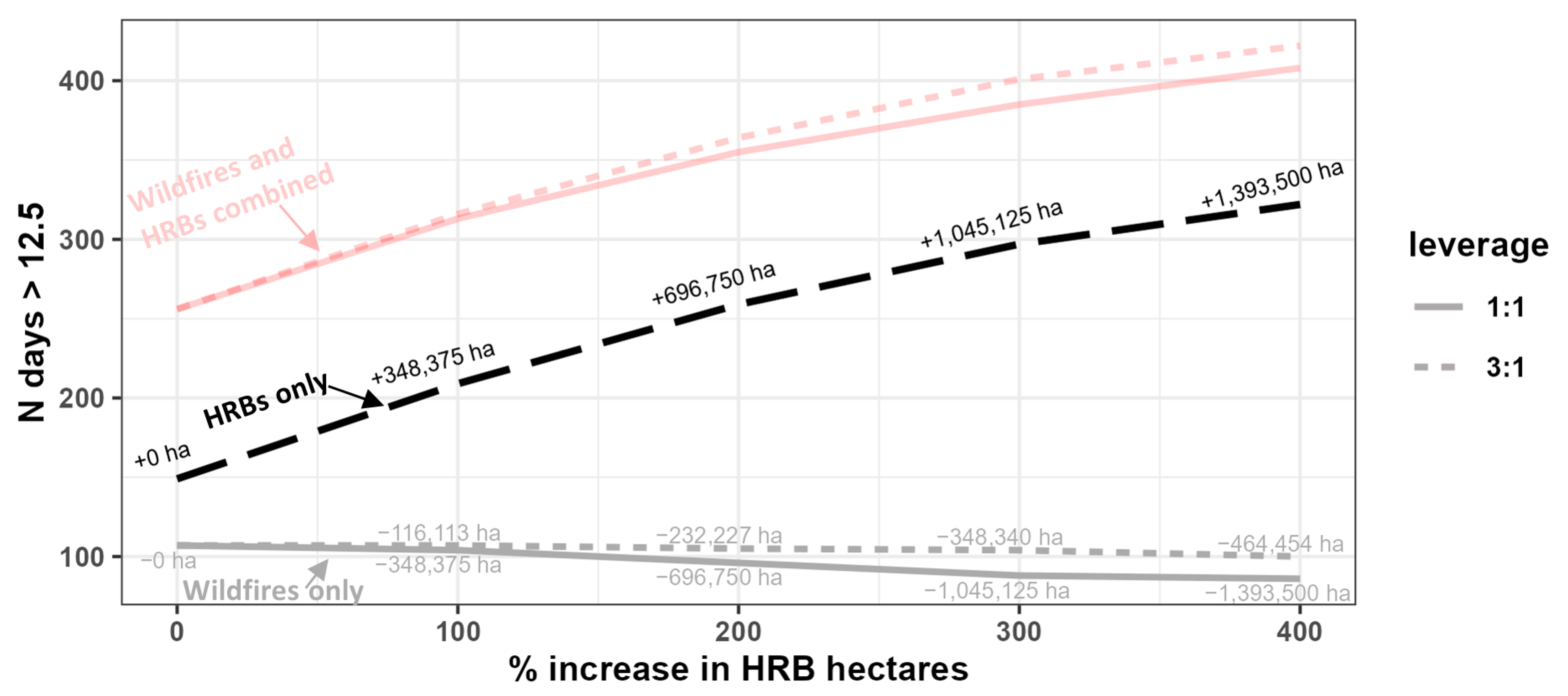
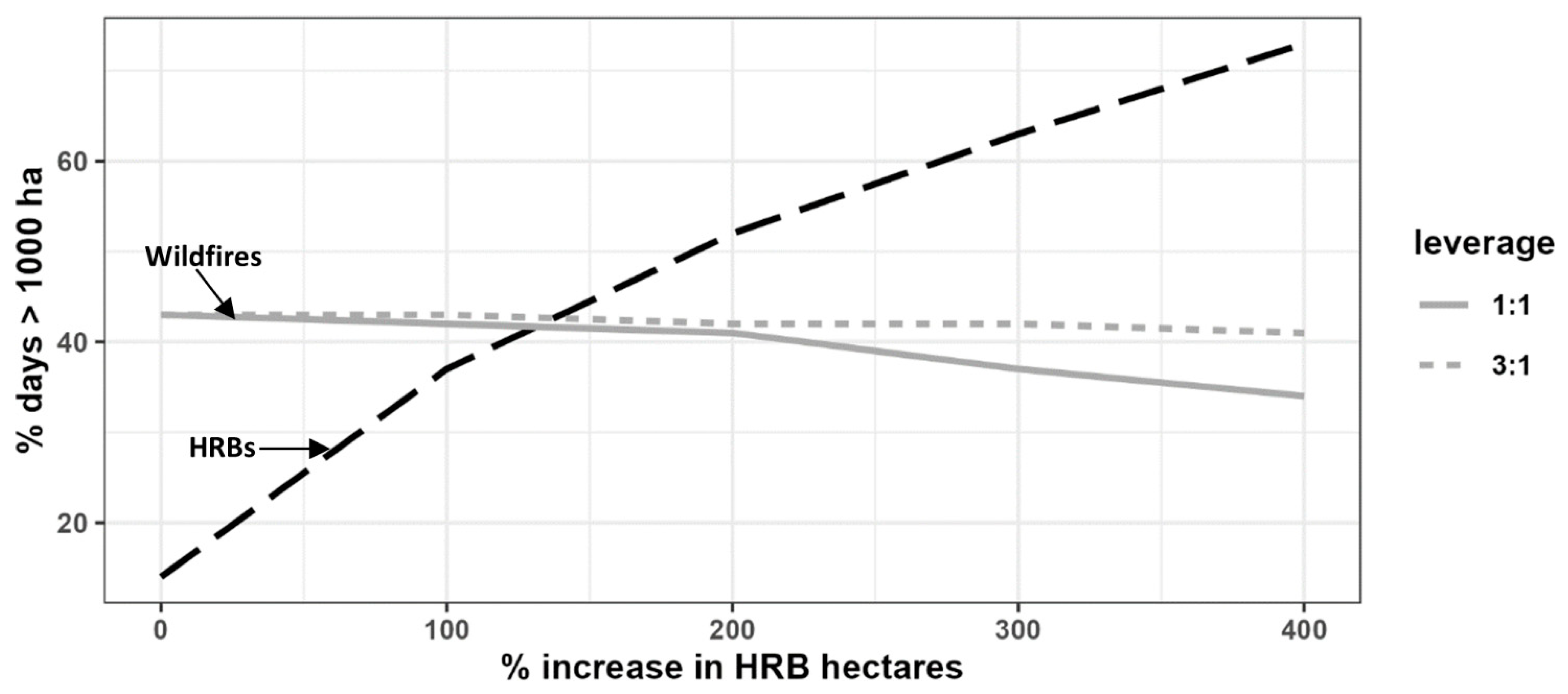
• Does increasing HRB treatment increase or decrease overall (HRB + wildfire) PM levels in Sydney (the trade-off between HRB and wildfires)?
• What is driving the nature of the trade-off?

We approach these questions using 24 h mean PM_2.5 observed at government air quality network stations and fire activity data from satellite sensors for the Sydney region.

2. Materials and Methods

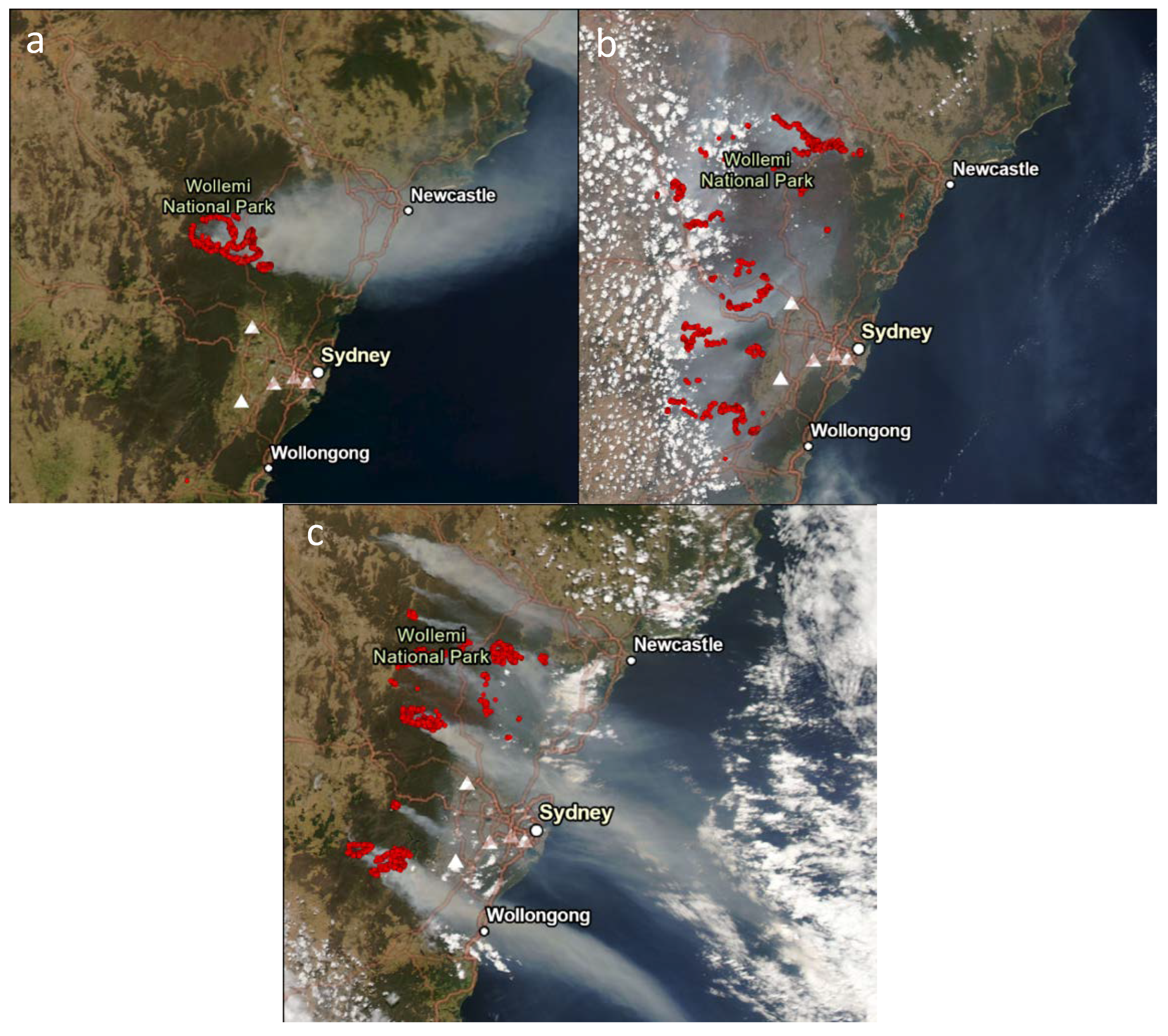
2.1. Study Area and Data

Our study used data generated for the analysis of Storey and Price [17], which developed a Bayesian model to predict HRB-related PM_2.5 across the Sydney basin as a function of daily weather and fire attributes. Here, in addition to HRBs, we also generated wildfire data for a comparison of wildfire and HRB smoke effects. More details on the data generation methods are in Storey and Price [17], but we provide a summary below.

Our study focused on Sydney, Australia, between 2012 and 2021. Specifically, we analysed active fires that occurred within 150 km of the Chullora air quality monitoring station (AQS). The region has a population of 5.2 million people (64% of the state of NSW), so air quality effects are concentrated here. We chose the 150 km radius because it captures the eucalypt forest-dominated Blue Mountains where landscape fires regularly occur, and this corresponds approximately with the radius that is most closely correlated with air quality in Sydney [18]. Sydney also has a permanent air quality monitoring network. Chullora AQS is centrally located among AQS with longer-term records in Sydney (Figure 1). Wildfires mostly burn in this region in the dry spring–summer periods, and HRBs are conducted in calm weather (mostly) during autumn or spring when dead fuel moistures are within a suitable range [1,19]. Both fire types have led to pollution events in the city that had high health costs [20,21].

We used VIIRS SNPP (Visible Infrared Imaging Radiometer Suite Suomi National Polar-Orbiting Partnership, [22]) satellite hotspots to identify days with active fires and total area of actively burning fires within the 150 km buffer for every day between 2012 and 2021, with our ‘day’ running from midday to midday as in Storey and Price [17]. For modelling, we excluded days in which no actively burning fires were detected by VIIRS, i.e., excluding days in which there was not at least one cluster of three or more hotspots detected [17]. This was to exclude days with only isolated hotspots, e.g., small wood piles or agricultural fires, and to exclude days without fires that may have had heightened PM_2.5 due to sources other than forest fires (e.g., dust, wood heater smoke). These very small fires that were excluded from our analysis (mainly small non-HRB and non-wildfires) were unlikely to substantially influence regional PM_2.5 observations because very small fires are generally associated with low observed PM_2.5 [15].

For the active fire days, we calculated the total regional fire area (i.e., total fire area for the 150 km buffer region) by intersecting all hotspots for 24 h with a 500 m by 500 m grid. The regional fire area was the total number of intersecting grid cells in the region (any cell intersecting >= 1 hotspot counted) × 25 ha. VIIRS SNPP acquires hotspots in the early afternoon and early morning (just after midnight). Early morning hotspots were grouped with the previous afternoon’s hotspots to ensure that our 24 h period for calculating fire area ran from midday to midday. Note that our use of VIIRS to identify active fire days provided a reliable method, although there would be occasions where the area was underestimated if fires were covered by dense clouds or small fires ignited and extinguished between VIIRS acquisition times (they were missed).

We used a simple definition to code a ‘fire type’ variable: all fires from March to September (inclusive) were HRB (as in Storey and Price [17]), and all fires from October to February were wildfires. This definition would place most fires in the right class, but some fires may have been misclassified (e.g., early wildfire, late HRB). We checked our fire type classification against the NSW National Parks and Wildlife Service Fire History [23]. The Fire History captures the location, ignition and end dates for fires. In our study period, 97% of the total NPWS classified HRB area ignited from March–September (i.e., our ‘HRB’ months), and 99% of the total NPWS classified wildfire area were from fires ignited from October to February (our ‘wildfire’ months). Note that we could not use the NPWS Fire History data for identifying active fire dates for our main analysis because it does not include a record of daily fire activity, only the final burnt area and ignition and end dates (though dates are sometimes missing).

We sampled ERA5 weather data from selected locations in the study area. ERA5 is made available by the European Centre for Medium-Range Weather Forecasts (ECMWF) and is a global gridded reanalysis data set that is generated based on model forecasts (ECMWF Integrated Forecast System) and observed data inputs [24]. We sampled hourly, 30 km resolution ERA5 surface parameters [25] that were found to be important in the previous analysis of PM_2.5 levels in Sydney associated with HRBs [17]. We sampled 2 m temperature and ventilation index (10 m wind speed * boundary layer height) over western Sydney, which was away from immediate coastal influence, and calculated 24 h (midday to midday) mean values for modelling. We also sampled 10 m U and V wind component variables along the coast near Sydney (centroid over Sydney International Airport) and calculated mean afternoon values to capture sea breezes. To capture inland wind patterns, we sampled U and V wind component variables over Katoomba, ~90 km inland in the Blue Mountains at 1000 m elevation, and calculated 24 h (midday to midday) mean values for modelling (see Storey and Price [17] for further details).

We extracted hourly PM_2.5 data from New South Wales government records available at https://data.airquality.nsw.gov.au/docs/index.html (accessed on 27 November 2021) for five stations in Sydney: Chullora, Liverpool, Camden, Richmond and Earlwood. These stations had records covering the start to the end of the study period, with the start defined by the first availability of VIIRS hotspots (2012) and the end in 2021. We calculated 24 h mean PM_2.5 values for the Sydney region by (1) calculating mean 24 h values for each station and (2) calculating the mean of the five 24 h station values. A 24 h period was from midday to midday to align with the cycle of fire activity and PM_2.5 impact, which in general is early afternoon ignition and smoke effects until the next morning. This is not always the case, particularly for large campaign fires (e.g., 2019–2020 Black Summer fires) that burn continuously but do fit most HRBs and wildfires. There are other sources of PM_2.5 that were not accounted for in our analysis, including vehicle exhaust, industrial sources and wood smoke from heating.

2.2. Statistical Modelling

Storey and Price [17] developed a Bayesian predictive model for HRB days with splines for the predictor variables. That work did not consider wildfire-related PM. Here, we instead used generalised linear modelling (GLM) for our analysis and compared HRB to wildfire-generated PM_2.5. We chose to use a GLM here to focus on the mean trends rather than capturing uncertainty, as with a Bayesian analysis. A Bayesian approach may be warranted for future analyses but was not required to explore the broad trends. Therefore, the model in Storey and Price [17] informed our selection of predictor variables, but here, we (1) fitted a generalised linear model to compare HRB and wildfire area effects and (2) predicted different burning scenarios using the models to explore the trade-off between wildfires and HRBs.

We fitted a GLM of 24 h mean PM_2.5 with an interaction between fire type and fire area using R statistical software [26]. We modelled PM_2.5 using a gamma GLM with a log-link function since values can only be positive and tend to follow a right-tailed distribution. Inspection of model residuals via the ‘DHARMa’ package (QQ plot, KR test, outlier test) [27] confirmed that this was an appropriate choice for our data.

Given that fire area effects were a main interest, and the effects would have a large influence on the subsequent trade-off analysis, we conducted an exploratory analysis to identify the best way to represent fire area in the models. This involved examination of scatter plots (area vs PM_2.5 by fire type) and simple models of PM_2.5 predicted by only fire area. We fitted linear models (separately by fire type) to different portions of the data to see if relationships were consistent over all fire sizes. We fitted linear models for data where the fire area was <2500 ha and over the whole data. The bulk of fire areas were <2500 ha (98% for HRB, 66% for wildfire), so this step allowed us to identify possible differences in the relationship between smaller fires (the bulk of the fires) and all data including the rarer large fires. We found vastly different ranges of fire area for HRBs vs wildfires in this exploratory analysis. In a simple linear model (with fire area expressed on the natural scale), fitted trends for wildfire and HRB area were similar when considering where the majority of the data was situated (fires < 2500 ha; Figure 2a,b). However, for wildfire days, there was a relatively small proportion of high-leverage data points (2500 ha to 82,800 ha) that substantially changed the fire vs PM_2.5 slope (Figure 2a). The simple linear model suggested a non-linear effect of fire area would be most appropriate in the models, so for the GLM, we log-transformed (base 10) the fire area variable. This transformation was also appropriate because there were no large HRB days to compare to (all HRB days < 5500 ha). Thus, the log transformation (a) better captures the relationship for the bulk of the data (smaller fire areas) and (b) captures potentially different per-hectare effects between large and small fire days (especially for wildfires).

We fitted a GLM to explore the effect of the fire area variables and determined if the effect differed between HRBs and wildfires. The model was fitted with log regional fire area, fire type, lagged PM_2.5, temperature, ventilation index and wind (U and V) along the coast and inland (Katoomba) [17]. We fitted the model with an interaction between fire type and fire area, and separate interactions between the U and V wind components [17]. Thus, the basic syntax for our GLM (gamma with log-link) was:

PM_2.5 = log10(fire area):fire type + Lag-PM_2.5 + temperature + ventilation index + coastalU:coastalV + inlandU:inlandV

(1)

Lagged PM_2.5 accounts for the influence of smoke and other pollutants that may remain in the area from the previous day, for example, on multi-day fires. It has also been found to be a strong predictor of current PM_2.5, so it is important for predictive accuracy_. Lagged PM_2.5 was calculated the same way as our dependent variable (24 h mean PM_2.5) except that it was for the prior 24 h period. We used the total regional fire area here to simplify the analysis instead of splitting fire area by direction from Sydney, as in Storey and Price [17]. As a post hoc check on our selection of a non-linear effect of fire area, we also fitted a Generalised Additive Model (GAM) using the same variables and interactions as the GLM, except that fire area was not transformed for the GAM and all variables were fitted with splines. Inspection of predicted effects plots from the GAM indicated that the log-transformation was a good approximation of the effect because, across the large range for wildfires, there was an initial steep rise in the effect on area on PM_2.5 that levelled out as fire area increased, albeit with a large degree of uncertainty due to a large scatter in the data (Figure 2c).

We explored the question of a trade-off between wildfire smoke and HRB smoke via an analysis using the model and a process to alter the modelling data to represent different scenarios. We split the data into an HRB set and a wildfire set. We first extracted the predictions from each set without altering the model data (0% change). We then increased the total HRB hectares by 100%, 200%, 300% and then 400% more than the actual area that occurred (i.e., 0%). For example, for a 100% increase in HRB area, we doubled the total area for each day in the HRB dataset and re-ran the predictions. All variables other than area were held as they were in the original model data. Our approach would reflect a strategy of increasing the area of HRBs that are planned but not increasing the number of days on which HRBs are planned. To analyse the trade-off, we applied leverage of 3:1, where three hectares of HRB burning reduces wildfire area by one hectare, which has been supported by research in the Sydney region and other landscapes [9,10]. Thus, in the wildfire dataset, we reduced the total area by an amount equal to one-third of the increase we applied to the HRB dataset (e.g., 1000 ha increase in HRB = 333.33 ha decrease in wildfire) and re-ran the predictions. We applied the decrease proportionally over each day in the wildfire dataset, so each wildfire day lost the same proportion of total area. States in Australia have different goals for daily PM_2.5, with the national reportable exceedance levels being >25 µgm⁻³ at a single AQS [28]. Since our mean PM_2.5 was calculated for 24 h from five stations, it represented a Sydney-wide mean PM_2.5. High values of the Sydney-wide PM_2.5 occur relatively rarely compared to a high value being recorded at just one station. Thus, we used a lower PM_2.5 value to summarise predictions for each scenario: we compared the number of days in each set where predicted PM_2.5 was >= 12.5 µgm⁻³, which the State of Victoria considers ‘Fair’ (or worse) air quality (<12.5 µgm⁻³ is ‘good’) [29]. This provided a better spread of data for modelling than if we used the 25 µgm⁻³: for example, only 17 of 597 HRB days were >25 µgm^−3, but 145 were >12.5 µgm⁻³. However, as an additional sensitivity step, we re-ran the trade-off analysis with a 25 µgm⁻³ threshold and also plotted changes to the median predicted PM_2.5 (Figure A1 and Figure A2).

We also ran additional trade-off analyses to test the sensitivity of (a) our use of a leverage of 3:1 and (b) our log transformation of fire area. For these analyses, we (a) used the main model (log-transformed fire area) to re-run the trade-off analysis with leverage of 1:1, i.e., 1 ha increase in HRB area equals 1 ha decrease in wildfire area (included in results), (b) re-ran the trade-off analysis using a GLM that contained non-transformed fire area (Figure A3 and Figure A4) and (c) re-ran the trade-off analysis using the GAM that was fitted during exploratory analysis (Figure A5). These steps help to identify aspects of our analysis that may have had a large influence on the results.

3. Results

3.1. Data Summary

In our study period from 2012 to 2021, we identified almost double the number of days when HRBs were actively burning (HRB days, 597 days) to days when wildfires were actively burning (wildfire days, 298 days). The HRB days had a much smaller total area: 348,375 ha for HRB days and 2,188,075 ha for wildfire days. For total area on HRB days, 98% of observations were <2500 ha (median = 350 ha, 95th centile = 1875 ha, maximum = 5550 ha). For wildfire days, 66% were below 2500 ha (median = 675 ha, 95th centile = 4214 ha, maximum = 8800 ha). The largest areas were recorded on wildfire days: 43% of wildfire days were >1000 ha (14% for HRB). Of the wildfire days > 5000 ha (n = 77), 22 were from the 2013–2014 fire season (including the State Mine fire), 1 was during February 2018 (‘695’ fire in Wollemi National Park), and 54 were from the 2019–2020 Black Summer bushfires [30].

3.2. Generalised Linear Modelling

For the GLM, lagged PM_2.5, log regional fire area, ventilation index and U component of coastal wind all had significant p-values (p < 0.001), while temperature and U component in Katoomba had p-values between 0.05 and 0.1. Fire type was not significant, and there was not a significant interaction between total area and fire type (Figure 3). The model explained 53.4% of the null model deviance. A table with coefficients for the model is in

Table A1. Model coefficients the model. d.e. = deviance explained. See Figure 3 in the main text for the matching effects plot.

Model	Term	Estimate	Std.Error	t Value	p Value
Total area (AIC = 5066, d.e = 53%)	intercept	1.2393	0.1423	8.7094	0
	lag PM2.5	0.0239	0.0019	12.7494	0
	ventilation index	−0.0001	0	−4.8575	0
	temperature	−0.0079	0.0048	−1.6578	0.0977
	log hectares all	0.3551	0.0486	7.3039	0
	fire type (WF)	0.1117	0.1649	0.6776	0.4982
	u10 coast	−0.0319	0.0081	−3.9601	0.0001
	v10 coast	−0.0099	0.0063	−1.5651	0.1179
	u10 Katoomba	0.0251	0.0138	1.8161	0.0697
	v10 Katoomba	−0.0362	0.0277	−1.3059	0.1919
	log hectares all:fire type (WF)	−0.0219	0.0578	−0.3794	0.7045
	u10 coast:v10 coast	−0.0002	0.0012	−0.137	0.8911
	u10 Katoomba:v10 Katoomba	−0.0076	0.0082	−0.9288	0.3532

.

3.3. Trade-Off

The model predicted 104 days of PM_2.5 > 12.5 for HRB and 120 days for wildfire for the model data (Figure 4). For days predicted to be >12.5 µgm⁻³ (0% increase in Figure 4), the median area for wildfires was 7425 ha, and for HRBs was 937 ha.

Increasing the total HRB area in the region increased the number of predicted days > 12.5 µgm⁻³ and reduced the number of wildfire days > 12.5 µgm⁻³ because leverage was applied. The model predicted that doubling (+100%) regional HRB area over the study period increased predicted days > 12.5 µgm⁻³ by 68, for a total of 172 days (Figure 4). Increasing regional HRB area by adding 200%, 300% and then 400% added 30 to 50 days > 12.5 µgm⁻³ for each scenario. The reduction in regional wildfire area in each step, assuming 3:1 leverage, resulted in only minor changes to the number of wildfire days predicted > 12.5 µgm⁻³: between 0 and 3 in each step in Figure 4. There were also only minor changes to the median predictions for wildfire under any scenario: between 0 and 400%, HRB median predicted PM_2.5 increased by 2.7 µgm⁻³, but wildfire reduced by only 0.4 µgm⁻³ (Figure A1). There were only minor differences in our results when leverage of 1:1 was applied for sensitivity testing (Figure 4), although there was a 1.4 µgm⁻³ change in median PM_2.5 with 1:1 leverage (Figure A1). When we applied predictions using a GLM (Figure A3 and Figure A4) and a GAM (Figure A5) that both had fire areas on the natural scale (not transformed), it similarly predicted a large increase in HRB days and a small decrease in wildfire days > 12.5 µgm⁻³. In re-running the analysis using a PM_2.5 threshold of 25 µgm⁻³ (and 3:1 leverage), results were similar in that there was a substantial increase in HRB days above the threshold but a negligible change to wildfire days above the threshold (Figure A2). However, two notable differences were a larger reduction in wildfire days above the threshold with 1:1 leverage and no rise (from 3 days predicted at 0% change) in HRB days above the threshold at a 100% increase in HRB area.

Under each scenario in our main trade-off analysis, there was a higher proportional change to regional area for HRBs compared to wildfires. A 100% increase in HRB ha would mean increasing total areas by 348,375 ha (i.e., 348,375 ha + 348,375 ha). Using leverage of 3:1, wildfire area would reduce by a third of that amount (348,375 ha/3= 116,125 ha). Additionally, 116,125 ha is only a ~5.3% change in wildfire area overall and each day in the data when applied proportionally. Through the scenarios (0% to 400%), many days with low regional HRB areas became days with large regional HRB areas, while large wildfire days remained large (Figure 5), suggesting there was more potential for change in predicted PM_2.5 among the HRB days. For example, the number of days with regional HRB area > 1000 ha grew from 85 to 435 (14% to 73% of days), but the number of days with regional wildfire area > 1000 ha only dropped from 127 to 123 (~43% of wildfire days) (Figure 5).

4. Discussion

Our first aim was to compare the effects of regional HRB and wildfire area on 24 h PM_2.5 in Sydney. There were no significant differences between wildfire and HRB area effects in the model, suggesting negligible differences exist when weather and the prior day’s PM_2.5 are accounted for. However, our trade-off analysis with the model suggested that although increasing regional HRB area would reduce regional wildfire area, it would probably lead to higher overall (wildfire + HRB) PM_2.5 pollution in Sydney. Our results apply to the Sydney region, but similar effects may occur in similar landscapes dominated by Eucalypt forests, although further research would be required to better understand the trade-off in other landscapes and vegetation.

The main reason for our result is that the effect of area was non-linear, and so was most sensitive to changes in regional fire area at the lower end of the scale. In other words, there was a greater per-hectare effect for smaller fire areas. In our data, HRB days had lower regional fire areas and were more common than wildfire days (mean regional HRB ha = 584, mean regional wildfire ha = 7343). Increasing the area amongst those days that initially had low regional HRB areas resulted in substantial increases in PM_2.5. Decreasing the area (by a few hundred or thousand hectares) amongst days those days that initially large regional wildfire area did not substantially change predicted PM_2.5. Moreover, at each step of our trade-off analysis, there were only small percentage changes to the regional wildfire areas amongst the initially large wildfire days, i.e., the days that had large regional areas remained large at each step. For example, from a 0 to 400% increase in regional HRB area, the percentage of HRB days > 1000 ha increased from 14% to 73%, but the percentage of wildfire days > 1000 ha was ~ 42% in all scenarios (Figure 5). This meant there were only small differences in predicted PM_2.5 from wildfires at each step due to the non-linear effect in the model.

The reasons for a non-linear relationship are not clear. However, a large contributor would be large burning areas that result in relatively low PM_2.5 (Figure 2a). We think that there are three likely contributors to this: smoke is lofted over the basin, smoke is blown in a different direction and/or smoke that enters the basin is blown away quickly. Firstly, because the power of the fire increases with size, it is likely that plumes are more frequently (and a greater proportion of the smoke is) lofted above the surface in large individual fires (Newcastle had low PM_2.5 in Figure 6a). Large individual fires likely contributed the most area when we recorded large regional fire areas in our data. There is evidence for plume lofting: radar analysis has shown plume top height to increase with the area of individual fires [13]. Secondly, there are occasions where very large regional fire areas were burning under wind patterns that shift smoke away from Sydney: e.g., easterlies blowing smoke inland (where PM probably increased at inland stations) (Figure 6b) or, in fires north of Sydney, westerlies blowing smoke directly out to sea (Figure 6a) [31]. Such scenarios may result in more pollution in other populated areas not captured in our analysis (we only used PM_2.5 in Sydney), such as Wollongong, Newcastle and Bathurst. Thirdly, while HRBs are generally conducted in low wind for safety reasons, wildfires are more likely to occur in windy weather that blows the smoke through Sydney and out to sea. This effect can be seen in Figure 6c, where the smoke plumes from the Black Summer fires on 5 December 2019 extended hundreds of kilometres offshore. Dispersal on this scale is not observed with smaller fires. Plumes under these strong winds can be narrow, meaning much of Sydney is not directly under a plume and smoke does not disperse across the basin (Figure 6c), as may happen under low winds and a sea breeze.

Several points should be noted in interpreting results. There was much scatter in the raw data (regional fire area vs PM_2.5, Figure 2), so the resulting model could not confidently predict individual events. However, the general trends our analysis captures are important to consider for fire management. The behaviour of our model here was dependent on log-transforming the fire area variable, but this was justified because the linear model in the exploratory analysis was strongly influenced by larger fire days and underestimated for smaller fire days. This problem was apparent when the modelling was repeated but restricted to wildfire days with small areas: the slope was 10 times steeper than for all wildfire days (Figure 2). We do not know if HRBs would conform to the same logarithmic pattern as wildfires if they had the same regional fire area range because there were no large HRB days. This may not be an important question because there is a practical limitation on the size and number of HRBs that can be conducted in a region because they are conducted under mild weather conditions, and fire agencies deploy fire crews to keep them contained, as opposed to wildfires which are uncontrolled and can burn under extreme weather over hundreds of thousands of hectares. It should also be noted that using a GAM (Figure A5) and a GLM (Figure A4) with a non-transformed area produced similar results for the trade-off.

Our results showed negligible differences in the per-hectare effect between HRB and wildfire days. Mainly, larger fire days had less per-hectare effect than smaller fire days. Previous research has aimed to understand differences in smoke production, transport and exposure by fire type. However, fire type has not consistently been a useful or the best available predictor of air-quality-related factors, including fuel consumption [11], PM_2.5 concentration from individual fires [15] and large particle plume top height [13], with fire area usually a more reliable predictor. Some studies have found large differences in the effect of wildfire and HRB fire area on air quality. Borchers-Arriagada et al. [16] found that HRBs had 1.2 times the health cost of wildfires regionally in New South Wales, Australia, but that increased to 4.6 times when two extensive wildfire seasons (summers of 2019–2020 and 2002–2003) that had a large influence on their model were included. In Navarro et al. [32], wildfire studies in the USA generally reported lower pollution levels than HRBs, but they attributed this to methodological differences: monitors were much closer to HRBs. A lack of consistent fire-type effect is probably because most HRBs and wildfires are small and probably burn under broadly similar weather (i.e., extreme fire weather is rare). Across NSW, ~70% of ‘wildfires’ in the NPWS fire history data between 2010 and 2020 were < 100 ha (~90% < 1000 ha). Price et al. [11] found considerable overlap in the types and amount of fuels consumed in individual HRBs and wildfires, suggesting they can have similar burning behaviour. The extreme end of fire behaviour distributions (largest areas, fastest spreading fires) are wildfires, but these are a minority of all fires. The outcome of this is that other fire characteristics (intensity, fuel amount, weather) that directly influence smoke production, transport and exposure are probably better than fire type for the prediction of air quality metrics [15]. Distance from a fire is also important for understanding PM_2.5 levels, with monitoring stations close to fires (<20 km) having higher PM_2.5 levels than those farther away [15,33], and HRBs (and their plumes) tend to be closer to urban areas where monitors are than wildfires [14,34].

We have provided evidence that increasing regional HRB area would increase the Sydney population’s total exposure to landscape fire-generated particulates. This needs strong consideration in HRB planning and implementation. There may be approaches to conducting HRBs that reduce particulate exposure, but further trans-disciplinary research is needed to evaluate these. This should include identifying the best weather conditions to conduct HRBs that will reduce smoke impact and how this restricts the number of days per year on which HRBs are possible. Our research suggests bigger HRBs would have less of a per hectare impact (particularly > 1000 ha) than small HRBs, so, for example, burning a 1000 ha burn on one day would be better than conducting four 250 ha fires over four days. However, this may conflict with other goals, i.e., burning a large HRB on a single day may require windier weather to ensure fire spread across the entire area, but this would make an escape more likely. The research will also need to consider the impact of changing HRB implementation PM_2.5 in other locations (e.g., west, north and south of Sydney) and on other risk factors, such as reducing wildfire spread risk near communities, and on the cost of implementation.

5. Conclusions

Understanding how landscape fires impact PM concentration and health in populated areas is a complex problem, but there is sufficient research to make some robust conclusions. Our model suggests that a hypothetical increase in HRB treatment would increase, rather than decrease, overall PM levels in Sydney. This will be critical to consider in the development of future HRB plans and must be further explored via future research and monitoring.

Because the timing and burning strategies of HRB are decided by fire managers, we hope that our research will improve managers’ abilities to plan burns to avoid the worst of the impacts. Our research suggests bigger HRBs (and large wildfires) would have less of a per-hectare impact on PM in Sydney than small HRBs, so a single large HRB may have less of an impact than a series of small burns. However, this is a very broad outcome, and other factors need further research, including the impact of different ignition and burning times (e.g., night burning vs day burning) and that this effect may differ depending on location in the world. The impact of smoke in other directions would also need to be considered (we did not consider Newcastle, Wollongong, Bathurst, etc.).

The processes driving our results have been partially explored in other research (fuel consumption, emission factors, plume dynamics, etc.), but much of the complexity, including how different factors interact, has not been resolved in this or other research. There is currently no highly reliable model of PM levels from landscape fires that captures the whole process. Ultimately, we need practical tools to assist fire managers in their choice of where, how and when to burn, in particular, to burn during conditions that achieve wildfire spread risk reduction but also avoid the worst pollution effects. Primarily, that is by avoiding weather conditions that trap air in the Sydney basin. Of course, this is not easy, partly because those conditions cannot reliably be forecast and partly because avoiding them leaves fewer available days when HRBs can safely be conducted. Our research helps progress towards this goal, but continued trans-disciplinary research is required to develop widely applicable operational models.

References

1. Bradstock, R.A.; Williams, R.J.; Gill, A.M. Flammable Australia: Fire Regimes, Biodiversity and Ecosystems in a Changing World; CSIRO Publishing: Collingwood, Australia, 2012; ISBN 0-643-10482-8. [Google Scholar]
2. Fernandes, P.M.; Botelho, H.S. A Review of Prescribed Burning Effectiveness in Fire Hazard Reduction. Int. J. Wildland Fire 2003, 12, 117–128. [Google Scholar] [CrossRef]
3. Carter, M.; Howard, T.; Haylock, K.; Philpotts, V.; Richards, J. Independent Investigation of the Lancefield-Cobaw Fire. Rep. Indep. Lancefield-Cobaw Fire Investig. Team 2015. Available online: https://www.ffm.vic.gov.au/__data/assets/pdf_file/0002/20000/Independent-investigation-into-Lancefield-Cobaw-fire.pdf (accessed on 27 November 2021).
4. Johnston, F.H.; Borchers-Arriagada, N.; Morgan, G.G.; Jalaludin, B.; Palmer, A.J.; Williamson, G.J.; Bowman, D.M.J.S. Unprecedented Health Costs of Smoke-Related PM2.5 from the 2019–20 Australian Megafires. Nat. Sustain. 2021, 4, 42–47. [Google Scholar] [CrossRef]
5. Matz, C.J.; Egyed, M.; Xi, G.; Racine, J.; Pavlovic, R.; Rittmaster, R.; Henderson, S.B.; Stieb, D.M. Health Impact Analysis of PM2.5 from Wildfire Smoke in Canada (2013–2015, 2017–2018). Sci. Total Environ. 2020, 725, 138506. [Google Scholar] [CrossRef] [PubMed]
6. Johnston, F.H.; Henderson, S.B.; Chen, Y.; Randerson, J.T.; Marlier, M.; Defries, R.S.; Kinney, P.; Bowman, D.M.; Brauer, M. Estimated Global Mortality Attributable to Smoke from Landscape Fires. Environ. Health Perspect. 2012, 120, 695–701. [Google Scholar] [CrossRef]
7. Jones, B.A.; McDermott, S.; Champ, P.A.; Berrens, R.P. More Smoke Today for Less Smoke Tomorrow? We Need to Better Understand the Public Health Benefits and Costs of Prescribed Fire. Int. J. Wildland Fire 2022, 31, 918–926. [Google Scholar] [CrossRef]
8. Williamson, G.; Bowman, D.; Price, O.; Henderson, S.; Johnston, F. A Transdisciplinary Approach to Understanding the Health Effects of Wildfire and Prescribed Smoke. Environ. Res. Lett. 2016, 11, 125009. [Google Scholar] [CrossRef]
9. Price, O.F.; Pausas, J.G.; Govender, N.; Flannigan, M.; Fernandes, P.M.; Brooks, M.L.; Bird, R.B. Global Patterns in Fire Leverage: The Response of Annual Area Burnt to Previous Fire. Int. J. Wildland Fire 2015, 24, 297–306. [Google Scholar] [CrossRef]
10. Price, O.F.; Bradstock, R.A. Quantifying the Influence of Fuel Age and Weather on the Annual Extent of Unplanned Fires in the Sydney Region of Australia. Int. J. Wildland Fire 2011, 20, 142–151. [Google Scholar] [CrossRef]
11. Price, O.F.; Nolan, R.H.; Samson, S.A. Fuel Consumption Rates in Resprouting Eucalypt Forest during Hazard Reduction Burns, Cultural Burns and Wildfires. For. Ecol. Manag. 2022, 505, 119894. [Google Scholar] [CrossRef]
12. Liu, X.; Huey, L.G.; Yokelson, R.J.; Selimovic, V.; Simpson, I.J.; Müller, M.; Jimenez, J.L.; Campuzano-Jost, P.; Beyersdorf, A.J.; Blake, D.R.; et al. Airborne Measurements of Western U.S. Wildfire Emissions: Comparison with Prescribed Burning and Air Quality Implications. J. Geophys. Res. Atmos. 2017, 122, 6108–6129. [Google Scholar] [CrossRef]
13. Price, O.F.; Purdam, P.J.; Williamson, G.J.; Bowman, D.M.J.S. Comparing the Height and Area of Wild and Prescribed Fire Particle Plumes in South-East Australia Using Weather Radar. Int. J. Wildland Fire 2018, 27, 525–537. [Google Scholar] [CrossRef]
14. Price, O.F.; Bradstock, R.A. The Spatial Domain of Wildfire Risk and Response in the Wildland Urban Interface in Sydney, Australia. Nat. Hazards Earth Syst. Sci. 2013, 13, 3385–3393. [Google Scholar] [CrossRef]
15. Storey, M.A.; Price, O.F. Statistical Modelling of Air Quality Impacts from Individual Forest Fires in New South Wales, Australia. Nat. Hazards Earth Syst. Sci. 2022, 22, 4039–4062. [Google Scholar] [CrossRef]
16. Borchers-Arriagada, N.; Bowman, D.M.J.S.; Price, O.; Palmer, A.J.; Samson, S.; Clarke, H.; Sepulveda, G.; Johnston, F.H. Smoke Health Costs and the Calculus for Wildfires Fuel Management: A Modelling Study. Lancet Planet. Health 2021, 5, e608–e619. [Google Scholar] [CrossRef]
17. Storey, M.A.; Price, O.F. Prediction of Air Quality in Sydney, Australia as a Function of Forest Fire Load and Weather Using Bayesian Statistics. PLoS ONE 2022, 17, e0272774. [Google Scholar] [CrossRef]
18. Price, O.F.; Williamson, G.J.; Henderson, S.B.; Johnston, F.; Bowman, D.M.J.S. The Relationship between Particulate Pollution Levels in Australian Cities, Meteorology, and Landscape Fire Activity Detected from MODIS Hotspots. PLoS ONE 2012, 7, e47327. [Google Scholar] [CrossRef]
19. Murphy, B.P.; Bradstock, R.A.; Boer, M.M.; Carter, J.; Cary, G.J.; Cochrane, M.A.; Fensham, R.J.; Russell-Smith, J.; Williamson, G.J.; Bowman, D.M. Fire Regimes of Australia: A Pyrogeographic Model System. J. Biogeogr. 2013, 40, 1048–1058. [Google Scholar] [CrossRef]
20. Broome, R.A.; Johnstone, F.H.; Horsley, J.; Morgan, G.G. A Rapid Assessment of the Impact of Hazard Reduction Burning around Sydney, May 2016. Med. J. Aust. 2016, 205, 407–408. [Google Scholar] [CrossRef]
21. Johnston, F.; Hanigan, I.; Henderson, S.; Morgan, G.; Bowman, D. Extreme Air Pollution Events from Bushfires and Dust Storms and Their Association with Mortality in Sydney, Australia 1994–2007. Environ. Res. 2011, 111, 811–816. [Google Scholar] [CrossRef] [PubMed]
22. Schroeder, W.; Oliva, P.; Giglio, L.; Csiszar, I.A. The New VIIRS 375m Active Fire Detection Data Product: Algorithm Description and Initial Assessment. Remote Sens. Environ. 2014, 143, 85–96. [Google Scholar] [CrossRef]
23. Department of Planning and Environment. NPWS Fire History—Wildfires and Prescribed Burns. Available online: https://datasets.seed.nsw.gov.au/dataset/fire-history-wildfires-and-prescribed-burns-1e8b6 (accessed on 1 January 2022).
24. Hersbach, H.; Bell, B.; Berrisford, P.; Hirahara, S.; Horányi, A.; Muñoz-Sabater, J.; Nicolas, J.; Peubey, C.; Radu, R.; Schepers, D.; et al. The ERA5 Global Reanalysis. Q. J. R. Meteorol. Soc. 2020, 146, 1999–2049. [Google Scholar] [CrossRef]
25. Hersbach, H.; Bell, B.; Berrisford, P.; Biavati, G.; Horányi, A.; Muñoz Sabater, J.; Nicolas, J.; Peubey, C.; Radu, R.; Rozum, I. ERA5 Hourly Data on Single Levels from 1979 to Present. Copernic. Clim. Change Serv. (C3S) Clim. Data Store (CDS) 2018, 10. [Google Scholar] [CrossRef]
26. R Core Team. R: A Language and Environment for Statistical Computing 2020; Scientific Research Publishing: Wuhan, China, 2020. [Google Scholar]
27. Hartig, F. DHARMa: Residual Diagnostics for Hierarchical (Multi-Level/Mixed) Regression Models. Ph.D. Thesis, University of Regensburg, Regensburg, Germany, 2022. [Google Scholar]
28. Australian Government National Environment Protection (Ambient Air Quality) Measure: F2021C00475; Commonwealth of Australia: Canberra, Australia, 2021.
29. State of Victoria, E.P.A. PM2.5 Particles in the Air | Environment Protection Authority Victoria. Available online: https://www.epa.vic.gov.au/for-community/environmental-information/air-quality/pm25-particles-in-the-air (accessed on 26 September 2022).
30. Filkov, A.I.; Ngo, T.; Matthews, S.; Telfer, S.; Penman, T.D. Impact of Australia’s Catastrophic 2019/20 Bushfire Season on Communities and Environment. Retrospective Analysis and Current Trends. J. Saf. Sci. Resil. 2020, 1, 44–56. [Google Scholar] [CrossRef]
31. Storey, M.A.; Price, O.F.; Fox-Hughes, P. The Influence of Regional Wind Patterns on Air Quality during Forest Fires near Sydney, Australia. Sci. Total Environ. 2023, 905, 167335. [Google Scholar] [CrossRef]
32. Navarro, K.M.; Schweizer, D.; Balmes, J.R.; Cisneros, R. A Review of Community Smoke Exposure from Wildfire Compared to Prescribed Fire in the United States. Atmosphere 2018, 9, 185. [Google Scholar] [CrossRef]
33. Price, O.F.; Forehead, H. Smoke Patterns around Prescribed Fires in Australian Eucalypt Forests, as Measured by Low-Cost Particulate Monitors. Atmosphere 2021, 12, 1389. [Google Scholar] [CrossRef]
34. Price, O.F.; Rahmani, S.; Samson, S. Particulate Levels Underneath Landscape Fire Smoke Plumes in the Sydney Region of Australia. Fire 2023, 6, 86. [Google Scholar] [CrossRef]
Figure 1. Map of the study area. The black circle is a 150 km buffer around Chullora air quality station. Red triangles are air quality stations used in the analysis. Chullora station (black-edged triangle) is the centre of the 150 km buffer. Green is forested area. Basemap© OpenStreetMap.
Atmosphere 14 01657 g001
Figure 2. Plots from an exploratory analysis of the shape of fire area vs PM2.5 effect. (a,b) are fire area derived vs mean PM2.5 linear model results. Equation of each linear model shown in text in plots. (a) Wildfire (Oct–Feb) hectares, (b) Hazard Reduction Burn (Mar–Sep) hectares. (a,b) contain a linear model fitted to all data in red and a linear model fitted to the majority of data (0 to 2500 ha) in orange. Note different x scales. (c) is the fire area effects plot from a GAM that was fitted post hoc with weather variables and a fire area–fire type interaction.
Atmosphere 14 01657 g002
Figure 3. Effects plots for regional fire area (hectares) from the generalised linear model. The regional fire area (hectares) was log-transformed (base 10) for the model. PM2.5 units are µgm−3. Predictions are within the range of the training data for each fire type. (a) shows the area burnt effect on log10 scale, (b) is back-transformed to natural/original scale, limited to 50,000 ha.
Atmosphere 14 01657 g003
Figure 4. Results of trade-off analysis. The plot shows the changes in the predicted number of days > 12.5 µgm−3 from increasing regional hazard reduction burn (HRB) area from 0% to 400% above the actual amount in model data. The number of days and hectare changes are over the whole study period (2012 to 2021). The black long-dash line is HRB days > threshold, and the grey lines at the bottom for wildfire days > threshold by leverage applied (see legend). Pink lines at the top are the total of WF and HRB days > threshold by scenario and leverage. Regional hectares change under each scenario shown in the text near the applicable line.
Atmosphere 14 01657 g004
Figure 5. % of total days with regional area > 1000 hectares for each increased HRB scenario in trade-off analysis and with different leverage applied for wildfires (grey lines). This demonstrates that under each scenario, there is a much more substantial increase in large HRB days (long-dashed black line) than there is a decrease in large wildfire days (grey lines, each with different leverage applied), i.e., many HRBs change from small to large but most large wildfire days are still large under each scenario, suggesting only minor changes for wildfire PM2.5 predictions.
Atmosphere 14 01657 g005
Figure 6. MODIS images from days with relatively low 24 h PM2.5, given the very large fires burning. Red points are VIIRS hotspots, and white triangles are monitoring stations used in our main analysis. (a) 13 Nov 2019 (24 h PM2.5 = 6 µgm−3), (b) 26 Dec 2019 (8 µgm−3) and (c) 1 Dec 2019 (30 µgm−3). (a) shows a large fire, but the smoke plume misses Sydney. In addition, PM2.5 was <10 µgm−3 in Newcastle, indicating the plume was lofted. (b) shows a very large fire area, but smoke is being blown inland under easterly winds. (c) shows very active fires with smoke, some of which enter Sydney, being blown out to sea by high winds. Images are available at https://worldview.earthdata.nasa.gov/ (accessed on 1 November 2021). All images are ~2 pm local time and ~400 km across.
Atmosphere 14 01657 g006
Disclaimer/Publisher’s Note: The statements, opinions and data contained in all publications are solely those of the individual author(s) and contributor(s) and not of MDPI and/or the editor(s). MDPI and/or the editor(s) disclaim responsibility for any injury to people or property resulting from any ideas, methods, instructions or products referred to in the content.