The Sensitivity of the Icosahedral Non-Hydrostatic Numerical Weather Prediction Model over Greece in Reference to Observations as a Basis towards Model Tuning

Abstract

The ICON (icosahedral non-hydrostatic) numerical weather prediction model (NWP)’s sensitivity is evaluated for the geographical area of Greece. As ICON model has recently been endorsed operationally by the Members of the COSMO (Consortium for Small-scale Modeling); this attempt is in line with the further understanding of the model features, especially in the considered domain, characterized by a complex orography as well as an almost equally partitioned land–sea surface area. An extraordinary number of 24 model parameters have been tested for the whole 2020 year in reference to 88 Greek meteorological stations, with regard to the standard synoptic meteorological variables of 2 m temperature, 2 m minimum and maximum temperatures, dew-point temperature, 10 m wind intensity and 12 h accumulated precipitation. For these variables, the model sensitivity is given in terms of the annual average of all stations for the fifth lead day of the model runs when the sensitivity is expected to reach its peak. It was found that there is a considerable impact regarding the minimum and maximum values for many of the examined parameters in reference to their default values, and consideration is given to a heuristic recommendation on the selection of the most sensitive parameters.

1. Introduction

The performance of local numerical weather prediction (NWP) models depends on various factors, like the applied numerical schemes, the accuracy of the initial conditions, the entreated domain, the resolution of the model grid and the integration time step. In contrast to the numerically resolved part of an NWP model, of special importance is the complexity of the model physics, which is usually addressed and controlled by many parameters. Several of these parameters can be tuned by the user within certain limits, in order to better adapt the model to the local features of the considered area. Many of these parameters are inter-related, where their number increases as the model development progresses. As a result, choosing the optimum values for this undertaking in order for the model to function at its best is fairly difficult. Estimating the model sensitivity of these factors is an important first step in overcoming this challenge [1,2,3,4,5,6,7,8]. In the present work, this trait is realized for the local version of ICON model (ICON-LAM), a state-of-the-art NWP model [9,10], for a considerably large number of 24 tunable parameters under the motivation to consider the most sensible ones in various model performance optimization techniques [4,7,11,12,13,14]. This effort lies within the frame of COSMO (Consortium for Small-scale Modeling) [15], with the objective to replace the currently operational common platform of the local ensemble prediction system (COSMO-LEPS) [16,17,18], based on the synonymous COSMO model, with a successor based on ICON model, which is currently used operationally by the Members of the Consortium individually. It is a part of the COSMO priority project PROPHECY (PRObabilistic Prediction at High-resolution with EnhanCed perturbation strategY) [19]. The major objective of this project is to coordinate the advancements needed to create a next generation of ensemble systems that permit convection based on the ICON model, while the creation and evaluation of model perturbation techniques is the primary research focus. Such progress will be vital in meeting the pressing needs for accurately predicting flood and flash flood events in Greece and the Mediterranean in general. This work is targeted towards the examination of the model sensitivity regarding the limit values of the many tunable parameters of the ICON NWP model. It complements other initiatives of critically examining other aspects of the model’s potential, like its space and/or time discretization associated with different model version implementations [20], the application of different physics schemes [6,21] and also its climate mode [22].

In the present work, the ICON model was performed for the full year of 2020 in a domain that covered the wider area of Greece, placing an emphasis over the central Mediterranean area, which is considered crucial to the strategy of the COSMO-LEPS project (Figure 1a). The ICON model version of the IMS (Israeli Meteorological Service) installed at the ECMWF (European Centre for Medium-Range Weather Forecasts) [23] was chosen, and five-and-a-half-day (132 h) runs, the forecast range of COSMO-LEPS, were completed with the ECMWF supercomputing system using resources provided by the HNMS (Hellenic National Meteorological Service). The parameter sensitivity was gauged in reference to the average values of temperature, mean sea-level pressure, wind and precipitation of 88 Greek meteorological stations averaged together. This effort lies in contrast to previous, more general works [1,8], where the sensitivity is referenced with regard to the area average of the default parameter runs instead of observations. It was driven by the relatively modest understanding of any similar objective realization of the NWP models of the COSMO in this complex area that is used operationally at the HNMS, or even in NWP in general. Furthermore, the wider area of Greece may be considered as one of the most representative areas of the Central Eastern Mediterranean regime.

The testing was performed practically for the last (fifth) day lead time, where the difference in the observations from the corresponding model values was expected to be the highest, highlighting the model sensitivity, as well as being in conformity with the goals of the COSMO-LEPS long-range forecast targeting. The influence of many of the parameters’ minimum and maximum values proved to be significant in relation to the observations allowing a heuristic but systematic, as well as quite cogent, recommendation of the most sensitive parameters.

2. Materials and Methods

The first critical step of our methodology was the choice of the ICON model parameters pertinent for evaluation. Their number was not specifically limited, but it was required that they cover practically all areas of the tuning of a numerical weather forecast model, i.e., turbulence, convection, cloud cover, sub-scale orography, grid-scale micro-physics, land and sea processes. They were selected, ranked and updated by ICON experts [24] according to their estimated significance and in close reference to the COSMO model [1]. Although this approach led to a substantial computational workload, it reflected a significant rationale within the COSMO and NWP in general, to supervise and obtain a more concrete idea of the model response to a notable number of parameters, without constraining their number, as was the case in other works focused towards model optimization purposes [11,12,13,14]. The extensive list of the parameters is presented in reference

Table 1. List of the 24 parameters (p01–p24) of the tested sensitivity based on their encoded names, interpretation and relevance (first column) as well as their test range (second column). The default values are denoted with bold characters as well as their recommended relevance, with [H] and [M] standing for high and medium, respectively. It should be noted that for p02 and p03, the minimum and default values coincide.

Parameter, Encoded Name (Meaning) Relevance: High [H]/Medium [M]	MIN, DEFAULT, MAX
p01: a_hshr (scale for the separated horizontal shear mode) [M]	0.1, 1.0, 2.0
p02: a_stab (stability correction of turbulent length scale factor) [M]	0.0, 0.0, 1.0
p03: alpha0 (lower bound of velocity-dependent Charnock param) [H]	0.0123, 0.0123, 0.0335
p04: alpha1 (scaling for the molecular roughness of water waves) [H]	0.1, 0.5, 0.9
p05: c_diff (length scale factor for vertical diffusion of TKE) [H]	0.1, 0.2, 0.4
p06: c_soil (evaporating fraction of soil) [H]	0.75, 1.0, 1.25
p07: capdcfac_et (extratropics CAPE diurnal cycle correction) [H]	0.0, 0.5, 1.25
p08: cwimax_ml (scaling for maximum interception storage) [H]	0.5 × 10−7, 1.0 × 10−6, 0.5 × 10−4
p09: entrorg (entrainment convection scheme valid for dx = 20 km) [H]	0.00175, 0.00195, 0.00215
p10: gkwake (low-level wake drag constant for blocking) [H]	1.0, 1.5, 2.0
p11: q_crit (normalized supersaturation critical value) [H]	1.6, 2.0, 4.0
p1 p12: qexc (test parcel ascent excess grid-scale QV fraction) [M]	0.0075, 0.0125, 0.0175
p13: rain_n0_factor (raindrop size distribution change) [H]	0.02, 0.1, 0.5
p14: rdepths (maximum allowed shallow convection depth) [H]	15000, 20000, 25000
p15: rhebc_land (RH threshold for onset of evaporation below cloud base over land) [M]	0.70, 0.75, 0.80
p16: rhebc_ocean (ibid over ocean) [H]	0.80, 0.85, 0.90
p17: rlam_heat_rat_sea (scaling of laminar boundary layer for heat and latent and heat fluxes over water (constant product)) [H]	(0.25,28.0), (1.0,7.0), (4.0,1.75)
p18: rprcon (precipitation coefficient conversion of cloud water) [H]	0.00125, 0.0014, 0.00165
p19: texc (excess value for temperature used in test parcel ascent) [M]	0.075, 0.125, 0.175
p20: tkhmin_tkmmin (common scaling for minimum vertical diffusion for heat–moisture and momentum) [H]	0.55, 0.75, 0.95
p21: box_liq (box width for liquid cloud diagnostic) [H]	0.03, 0.05, 0.07
p22: box_liq_asy (liquid cloud diagnostic asymmetry factor) [H]	2.0, 3.5, 4.0
p23: tur_len (asymptotic maximal turbulent distance (m)) [H]	250, 300, 350
p24: zvz0i (terminal fall velocity of ice) [H]	0.85, 1.25, 1.45

, as in [8], and was a product of extensive internal discussions and considerations among ICON model experts. In this dense yet convenient setup, the encoded names of the parameters, along with a hint towards their meaning and their estimated degrees of significance (H, M standing for high and medium, respectively), is given in correspondence to the more detailed list [24]. Following this table, to avoid complexities regarding the nomenclature arising from their big number, the parameters are referenced simplistically as p01–p24 throughout the text, while their meaning is addressed to those of particular importance the first time they are encountered. Practically, this catalogue covers the essence of the model physical parameterization schemes associated with the following:

• Turbulence (p01, p02, p03, p04, p05, p11, p17, p20, p23);
• Land processes (p06, p08);
• Convection (p07, p09, p12, p14, p15, p16, p18, p19);
• Subscale orography tuning (p10);
• Grid-scale microphysics (p13, p24);
• Cloud cover (p21, p22).

All the parameters were tried over a domain covering the more extensive area of Greece within the Central Mediterranean (Figure 1a) for the entire year of 2020. Forty-seven model runs were performed for every case, with one referring to the default parameter setup, and forty-six corresponding to the replacement of one parameter with its minimum and maximum parameter values (i.e., p01–p24 of Table 1). It should be noted that for parameters p02 and p03, their minimum values coincided with their default values.

The Integrated Forecasting System (IFS) [25] operational forecast was used (in 3 h intervals) to drive the ICON model, which was set up by the Israeli Meteorological Service (IMS) at the former High-Performance Facility (HPCF) of the European Center for Medium-Range Forecasts (ECMWF) [26].

Moreover, due to the motivation of this effort towards the application of the model as a sequence to COSMO-LEPS [17,18], the forecast range of the deterministic ICON model was extended to 132 h on a 6.5 km horizontal grid mesh, as in the currently operational COSMO-LEPS. The exceptional computational cost from the resulting number of approximately 17,000 computer runs, the equivalent of a single run of more than two and a half centuries, placed a constraint on the size of the domain of integration (Figure 1a) that covered the wider area of Greece and Italy. The model output was stored at the ECMWF’s file storage system (ECFS) [27].

As a main feature, this domain includes equally partitioned marine and land areas with considerable orographic variability that made it particularly suitable for the goal of this work to highlight the relative sensitivities of all the parameters under consideration. In this work, the testing for sensitivity of the ICON model was performed over a total of 850,000 synoptic observations for the 88 Greek meteorological stations considered (Figure 1b). The observations refer to the standard synoptic meteorological variables of mean sea-level Pressure (MSLP), 2 m temperature (T2m), maximum and minimum 2 m temperature (T2m_min, T2m_max), dew-point temperature (Td2m), 12 h accumulated precipitation (TOTPREC) and 10 m wind intensity (W10m). The testing was performed practically for the fifth lead day (97th to 117th h) of the 132 h runs, where the difference in observations from the model values was expected to be at its climax, highlighting the model sensitivity. Regarding T2m_min and T2m_max, the observations were available for 47 stations instead of the 88 available ones for the other variables.

3. Results

The sensitivities (S) are presented via the averages of the variables <V> for the model runs associated with the minimum and maximum parameter values (p) with the corresponding recorded values at the meteorological stations. Over this period, these differences are expected to be at their peak as they fall at the end of the forecast period. These sensitivities are displayed in Figure 2, Figure 3, Figure 4 and Figure 5 for the whole year of 2020 and are defined as

$${ S}_{p<V>}\left(\%\right)=100·\left(\frac{{<V>}_{p_{model}}-{<V>}_{observed}}{{<V>}_{observed}}\right)$$

(1)

Along these figures, the sensitivities are displayed with purple and orange colors for the minimum (pi_min) and maximum (pi_max) parameter values alternatively for almost all the parameters, with the exception of the runs with the default values (blue) and p02_max and p03_max (red), because for these parameters, the minimum value runs coincide with the default parameter runs. A horizontal blue line also starts from the sensitivity value of the run with the default parameters to better compare it visually with the sensitivity of the other parameters. The graphs are completed with the average value of the considered meteorological variable observations, denoted in green boxes.

3.1. MSLP Sensitivities

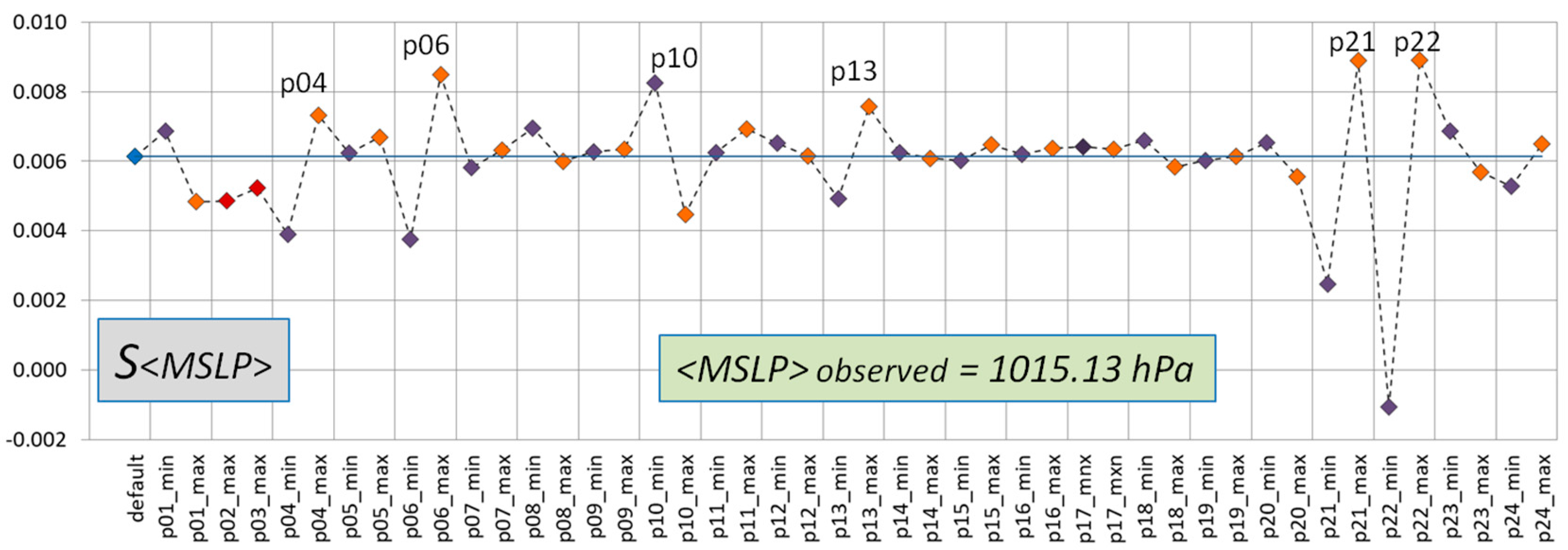
The order of the mean sea-level pressure sensitivities (S_<MSLP>) is ~10⁻³%, and the meteorological variable is sensitive to several parameters (Figure 2). With the exception of the most sensitive parameter, p22-min (liquid cloud diagnostic asymmetry factor), all sensitivities are positive, practically meaning that the model overestimates MSLP on average.

However, at least for the most sensitive parameters (p04, p06, p10, p13, p21, p22), denoted heuristically on the graph and in

Table 2. List of the meteorological variables over the corresponding parameters that display the greatest sensitivity as it can be inferred heuristically from Figure 2, Figure 3, Figure 4 and Figure 5 and over the 5th lead day of the model runs, and in reference to observations. The most sensitive parameters for every meteorological variable are addressed with bold-faced characters.

Met. Variables	Obs. Avg.	Order of S (%)	Most Sensitive Parameters
MSLP	1015.13 hPa	10−3	p04, p06, p10, p13, p21, p22
T2m	17.95 °C	10−1	p01, p06, p13, p17, p20, p22
T2m_min	12.92 °C	10	p01, p06, p10, p17, p20, p21, p22
T2m_max	22.23 °C	1	p06, p17, p21, p22
Td2m	10.68 °C	1	p04, p06
TOTPREC	0.98 mm	10	p04, p07, p09, p13, p14
W10m	6.52 Knots	5	p10

, their minimum and maximum values lie on the opposite sides of the blue line referring to the default parameter runs as expected; nevertheless, their positions are not symmetrical to the line. It is interesting to note that this particular feature remains in all the meteorological variables considered. From the heuristic standpoint, and at least for the most sensitive parameters, this feature shows that the sensitivity of the default value of this parameter is expected to be between the sensitivities of its limit values.

3.2. T2m, T2m_min, T2m_max and Td2m Sensitivities

The various temperature sensitivities were evaluated by considering units in degrees Celsius (°C) instead of the more natural Kelvin (K) in order to enhance the corresponding scale in the subsequent graphs and address the remarks more directly. In Equation (1), this option was acceptable due to the positive values of the considered average temperatures when they are expressed in °C.

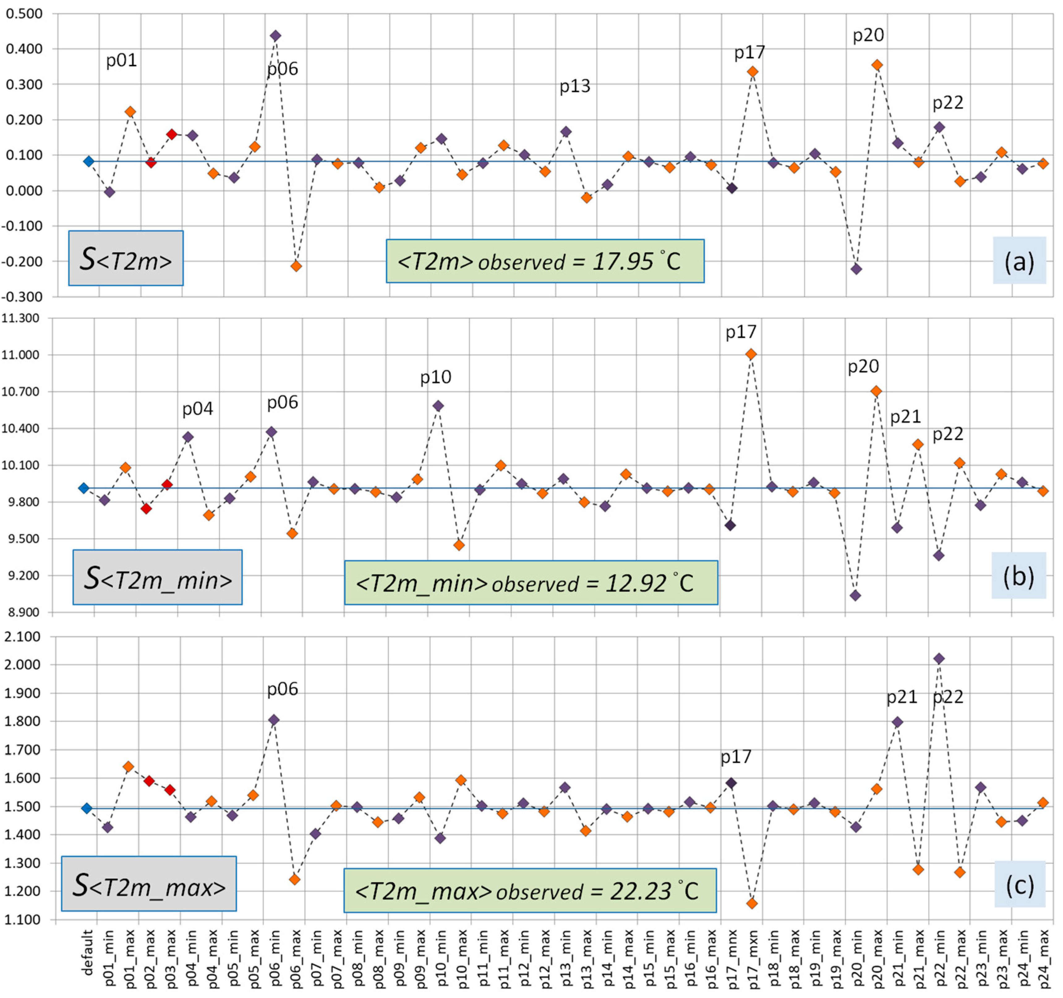
For 2 m temperature (Figure 3a), the order of sensitivities (S_<T2m>) is ~10⁻¹%, and almost all of them are positive, meaning that, on average, the 2 m temperatures are overestimated by the model. This feature is the same for the minimum and maximum 2 m temperatures, as shown in Figure 3b and Figure 3c respectively, where the order of the corresponding sensitivities (S_{<T2m_min>}) and (S_{<T2m_max>}) are ~10% and ~1%, respectively. The relative large order of S_{<T2m_min>} should be attributed to the fact that the units of °C used raise the value of the denominator significantly in Equation (1), and also that the minimum T2m values are relatively more overestimated by the model.

The more sensitive parameters regarding 2 m temperature are p01, p06, p13, p17, p20 and p22, with p06 (evaporating fraction of soil) and p20 (common scaling for minimum vertical diffusion for heat–moisture and momentum) clearly being the most sensitive ones (Figure 3a). Slightly different are the more sensitive parameters regarding minimum 2 m temperature (Figure 3b), i.e., p01, p06, p10, p17, p20, p21 and p22, with p17 (scaling of laminar boundary layer for heat and latent heat fluxes over water) and p20 being the most sensitive ones. As for the maximum 2 m temperature (Figure 3c), the more sensitive parameters are relatively reduced to p06, p17, p21 (box width for liquid cloud diagnostic) and p22, with all of them displaying approximately the same sensitivity.

The sensitivity of T2m, T2m_min and T2m_max to modestly different parameters might be due to the different physical processes acting, but also to the fact that T2m_min and T2m_max were independently observed in a subset of 47 stations out of the 88, as was mentioned at the end of Section 2.

For the dew-point temperature (Td2m) (Figure 4), there is a substantial reduction in the more sensitive parameters to practically only two, i.e., p04 (scaling for the molecular roughness of water waves) and p06. The sensitivity of the former parameter is an interesting feature and might be attributed to the fact that the considered stations are distributed in a widely different geomorphology, with an emphasis on coastal areas or located on islands. It is worth noting that p04 displays significant sensitivity to most of the other meteorological variables examined. The sensitivities for Td2m are of the order of 1% and are rather balanced between positive and negative values.

3.3. TOTPREC Sensitivities

All sensitivities regarding precipitation (Figure 5) are negative and of order ~10%; consequently, precipitation is clearly underestimated with the model even though it is sensitive to many parameters, highlighting the complexity of the issue [28].

The relatively more sensitive parameters are p04, p07 (extra-tropics CAPE diurnal cycle correction), p09 (entrainment convection scheme valid for dx = 20 km), p13 (raindrop size distribution change) and p14 (maximum allowed shallow convection depth), with p07 as the most sensitive one. As it was expected, these parameters are related to convection (p07, p09 and p14) but also to turbulence (p04) and grid scale microphysics (p13), highlighting the inter-relation among the different physical processes.

3.4. W10m Sensitivities

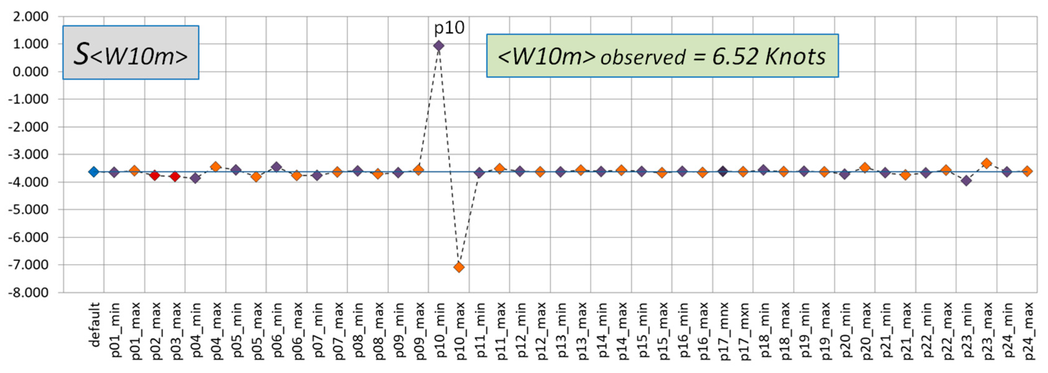
The sensitivities of the 10 m wind intensity (Figure 6) revealed a very important feature. Practically, only p10 (low-level wake drag constant for blocking) displays any considerable sensitivity of a relatively large value of order ~5%. They are all negative, with the exception of p10_min, which is positive. This means that in the considered model default setup, the W10m was underestimated, and an optimum parameter could be sought towards smaller parameter values. Indeed, in the updated configuration of the ICON model [21], it is mentioned that the German Meteorological Service (DWD) uses p10_min = 0.25 instead of the default value of 1.5 used in this work, which is generally recommended.

4. Discussion

Although the endeavor to address the sensitivity of such a large number of parameters in reference to the synoptic observations over such a complex domain as Greece looked overly challenging, it turned out that it was manageable within a straightforward and consistent framework. This feature may be considered to be a very positive aspect of the presented methodology in support of the model users and developers that favor the option to obtain a fast and clear vision of the model response to the many complexities regarding its parameterization. Indeed, such an undertaking can be taken by meteorological services, companies or institutes that run NWP models and routinely provide or have access to these standard synoptic meteorological variables.

The outcomes are summarized in Table 2, where the more sensitive parameters are displayed in the fourth column, along with the most sensitive ones depicted in bold characters. These parameters are marked heuristically, as they are rather clearly highlighted from Figure 2, Figure 3, Figure 4, Figure 5 and Figure 6. Their total number is constrained to 12 (p01, p04, p06, p07, p09, p10, p13, p14, p17, p20, p21 and p22), while the number regarding the most sensitive parameters is further limited to only eight, as it is denoted with bold letters in the previous parenthesis. In respect of this trend comes also one of the most important elements of this work, the overall development of a fairly straightforward and systematic way to choose the most sensitive or suitable parameters towards the employment of model optimization methods.

From a more technical standpoint, the order of the sensitivities for the different meteorological variables falls well within the observation accuracy, placing some limitations on what can be expected regarding the optimization of the model, at least for the specific region of application. In this case, for example, the underestimation of the average precipitation for all parameter limits most probably cannot change for any parameter combination; thus, further development is needed in the physics of the model. For 10 m wind intensity, on the other hand, it was only one parameter (p10_min) that showed positive sensitivity, making it rather straightforward to place a preferable value closer to it in preference to the default one, a feature that is also well undertaken by the DWD. It is worth mentioning that the most sensitive parameters practically referred to all the categories of the physical processes listed above. Consequently, the challenge to examine such a large number of parameters covering a broad spectrum of physical processes was rightly justified.

5. Conclusions and Prospects

In this work, an effort towards a systematic ranking of the model sensitivities was addressed in reference to an extensive set of observations for the area of Greece for a very large number of 24 model parameters. The study period was the complete year of 2020, and the sensitivities were evaluated for the fifth lead day of the model run, when they were expected to have their highest value. A critical motivation behind this heavy computational task was to investigate the possibility to address the most sensitive parameters via a methodical, comprehensive and applicable framework. In our previous works [11,12,13,14] of COSMO NWP model calibration via a meta-model, such a limitation to no more than five parameters was practically forced due to the computational cost, but also the algorithmic complexities from the dependence of these parameters to each other. In contrast to this effort, this crucial task was carried out heuristically under extensive discussion with model experts.

Due to the scope of examining a vast number of model parameters and the consequent exceptional computational task, the sensitivity was considered regarding minimum and maximum parameter values. The examination of intermediate values is expected to play an important role when this technique is applied to model optimization upon the most sensitive parameters [14]. As a follow-up, there was always the concern as to whether the most sensitive parameters had been selected and consequently, if the resulting performance optimization was the best possible one. It turned out that, via the presented procedure, it is possible to mark the most sensitive parameters in a reliable and visually transparent way.

This action of ranking the parameter sensitivity is expected to facilitate the development of model optimization methodologies like stochastic perturbative ensemble techniques [29,30], one of PROPHECY’s [19] main goals, or stepwise tuning [31,32].

Practically, Big Data [33] were produced from the exceptional number of model runs, compelled by the vast amount of observations used for a relatively little-studied area like Greece. This feature makes this work a good candidate for applications in the areas of current innovative technologies like artificial intelligence and/or machine learning that are taking a pivotal role in NWP and meteorology in general [34,35,36].

Although the ICON model was used as a prototype, the methodology can be applied and modified to any NWP model. Such a procedure is expected to play an important role in which parameters to consider in model performance optimization techniques in support of the criteria that are generally based on the experience of the model experts and/or extensive testing. The application of the methodology to the domain of Greece was a very critical part of the work, as this complex area is little studied regarding NWP model sensitivity, especially with respect to observations over such an extensive time period.

This work is expected to act as a benchmark towards further ICON model investigations, like seasonal targeted analysis applied to areas with specific climatological characteristics or other geophysical considerations.

References

1. Avgoustoglou, E.; Voudouri, A.; Carmona, I.; Bucchignani, E.; Levi, Y.; Bettems, J.-M. A Methodology Towards the Hierarchy of COSMO Parameter Calibration Tests Via the Domain Sensitivity Over the Mediterranean Area. COSMO Tech. Rep. 2020, Volume 42. Available online: https://www.cosmo-model.org/content/model/cosmo/techReports/docs/techReport42.pdf (accessed on 22 October 2023).
2. Baki, H.; Chinta, S.; Balaji, D.; Srinivasan, B. Determining the sensitive parameters of the Weather Research and Forecasting (WRF) Model for the simulation of tropical cyclones in the Bay of Bengal using global sensitivity analysis and machine learning. Geosci. Model Dev. 2022, 15, 2133–2155. [Google Scholar] [CrossRef]
3. Campos, T.B.; Sapucci, L.F.; Lima, W.; Silva Ferreira, D. Sensitivity of Numerical Weather Prediction to the Choice of Variable for Atmospheric Moisture Analysis into the Brazilian Global Model Data Assimilation System. Atmosphere 2018, 9, 123. [Google Scholar] [CrossRef]
4. Kim, S.-M.; Kim, H.M. Effect of observation error variance adjustment on numerical weather prediction using forecast sensitivity to error covariance parameters. Tellus A 2018, 70, 1492839. [Google Scholar] [CrossRef]
5. Merja, H.; Tölle, M.H.; Churiulin, E. Sensitivity of Convection-Permitting Regional Climate Simulations to Changes in Land Cover Input Data: Role of Land Surface Characteristics for Temperature and Climate Extremes. Front. Earth Sci. Sec. Atmos. Sci. 2021, 9, 722244. [Google Scholar] [CrossRef]
6. De Lucia, C.; Bucchignani, E.; Mastellone, A.; Adinolfi, M.; Montesarchio, M.; Cinquegrana, D.; Mercogliano, P.; Schiano, P. A Sensitivity Study on High Resolution NWP ICON—LAM Model over Italy. Atmosphere 2022, 13, 540. [Google Scholar] [CrossRef]
7. Marsigli, C. Final report on priority project SREPS (Short Range Ensemble Prediction System). COSMO Tech. Rep. 2009, 13. [Google Scholar] [CrossRef]
8. Avgoustoglou, E.; Shtivelman, A.; Khain, P.; Marsigli, C.; Levi, Y.; Cerenzia, I. On the Seasonal Sensitivity of ICON Model. COSMO Newsl. 2023, Volume 22. Available online: http://www.cosmo-model.org/content/model/documentation/core/default.htm (accessed on 22 October 2023).
9. Zängl, G.; Reinert, D.; Rípodas, P.; Baldauf, M. The ICON (ICOsahedral Non-hydrostatic) Modelling framework of DWD and MPI-M: Description of the non-hydrostatic dynamical core. Q. J. R. Meteorol. Soc. 2015, 141, 563–579. [Google Scholar] [CrossRef]
10. Prill, F.; Reinert, D.; Rieger, D.; Zängl, G. ICON Tutorial: Working with the ICON Model; Deutscher Wetterdienst: Offenbach, Germany, 2020. [Google Scholar]
11. Avgoustoglou, E.; Carmona, I.; Voudouri, A.; Levi, Y.; Will, A.; Bettems, J.M. Calibration of COSMO Model in the Central-Eastern Mediterranean area adjusted over the domains of Greece and Israel. Atmos. Res. 2022, 279, 106362. [Google Scholar] [CrossRef]
12. Voudouri, A.; Avgoustoglou, E.; Carmona, I.; Levi, Y.; Bucchignani, E.; Kaufmann, P.; Bettems, J.M. Objective Calibration of Numerical Weather Prediction Model: Application on Fine Resolution COSMO Model over Switzerland. Atmosphere 2021, 12, 1358. [Google Scholar] [CrossRef]
13. Voudouri, A.; Khain, P.; Carmona, I.; Avgoustoglou, E.; Kaufmann, P.; Grazzini, F.; Bettems, J.M. Optimization of high resolution COSMO Model performance over Switzerland and Northern Italy. Atmos. Res. 2018, 213, 70–85. [Google Scholar] [CrossRef]
14. Voudouri, A.; Khain, P.; Carmona, I.; Bellprat, O.; Grazzini, F.; Avgoustoglou, E.; Bettems, J.M.; Kaufmann, P. Objective calibration of numerical weather prediction Models. Atmos. Res. 2017, 190, 128–140. [Google Scholar] [CrossRef]
15. Consortium for Small-Scale Modeling. Available online: https://www.cosmo-Model.org (accessed on 22 October 2023).
16. COSMO Limited-Area Ensemble Prediction System. Available online: https://www.cosmo-Model.org/content/tasks/operational/cosmo/leps/default.htm (accessed on 22 October 2023).
17. Montani, A.; Cesari, D.; Marsigli, C.; Paccagnella, T. Seven years of activity in the field of mesoscale ensemble forecasting by the COSMO-LEPS system: Main achievements and open challenges. Tellus A 2011, 63, 605–624. [Google Scholar] [CrossRef]
18. Tomasso, D.; Marsigli, C.; Montani, A.; Nerozzi, F.; Paccagnella, T. Calibration of Limited-Area Ensemble Precipitation Forecasts for Hydrological Predictions. Mon. Weather Rev. 2014, 142, 2176–2197. [Google Scholar] [CrossRef]
19. COSMO Priority Project PROPHECY. Available online: http://www.cosmo-model.org/content/tasks/priorityProjects/prophecy/pp-prophecy.pdf (accessed on 22 October 2023).
20. Crueger, T.; Giorgetta, M.A.; Brokopf, R.; Esch, M.; Fiedler, S.; Hohenegger, C.; Kornblueh, L.; Mauritsen, T.; Nam, C.; Naumann, A.K.; et al. ICON-A, The Atmosphere Component of the ICON Earth System Model: II. Model Evaluation. J. Adv. Model. Earth Syst. 2018, 10, 1638–1662. [Google Scholar] [CrossRef]
21. Khain, P.; Shpund, J.; Levi, Y.; Khain, A. Warm-phase spectral-bin microphysics in ICON: Reasons of sensitivity to aerosols. Atmos. Res. 2022, 279, 106388. [Google Scholar] [CrossRef]
22. Van Pham, T.; Christian Steger, C.; Rockel, B.; Keuler, K.; Kirchner, I.; Mertens, M.; Rieger, D.; Zängl, G.; Früh, B. ICON in Climate Limited-area Mode (ICON release version 2.6.1). Geosci. Model Dev. 2021, 14, 985–1005. [Google Scholar] [CrossRef]
23. Khain, P.; Shtivelman, A.; Muskatel, H.; Baharad, A.; Uzan, L.; Vadislavsky, E.; Amitai, E.; Meir, N.; Meerson, V.; Levi, Y.; et al. Israel uses ECMWF supercomputer to advance regional forecasting. ECMWF Newsl. 2022, 171, 29–35. [Google Scholar]
24. ICON Model Parameters Suitable for Model Tuning. Available online: https://www.cosmo-model.org/content/support/icon/tuning/icon-tuning.pdf (accessed on 22 October 2023).
25. ECMWF Integrated Forecasting System. Available online: https://www.ecmwf.int/en/forecasts/documentation-and-support/changes-ecmwf-Model (accessed on 22 October 2023).
26. Hawkins, M.; Isabella Weger, I. Supercomputing at ECMWF. ECMWF Newsl. 2015, 32–38. [Google Scholar]
27. ECMWF’s File Storage System. Available online: https://confluence.ecmwf.int/display/UDOC/ECFS+user+documentation (accessed on 27 October 2023).
28. Singh, S.; Kalthoff, N.; Gantner, L. Sensitivity of convective precipitation to model grid spacing and land-surface resolution in ICON. Q. J. R. Meteorol. Soc. 2021, 147, 2709–2728. [Google Scholar] [CrossRef]
29. Puh, M.; Keil, C.; Gebhardt, C.; Marsigli, C.; Hirt, M.; Jakub, F.; Craig, G.C. Physically based stochastic perturbations improve a high-resolution forecast of convection. Q. J. R. Meteorol. Soc. 2023, 1–11. [Google Scholar] [CrossRef]
30. Ju-Hye Kim, J.-H.; Jiménez, P.A.; Sengupta, M.; Dudhia, J.; Yang, J.; Alessandrini, S. The Impact of Stochastic Perturbations in Physics Variables for Predicting Surface Solar Irradiance. Atmosphere 2022, 13, 1932. [Google Scholar] [CrossRef]
31. Ma, P.-L.; Harrop, B.E.; Larson, V.E.; Neale, R.B.; Gettelman, A.; Morrison, H.; Wang, H.; Zhang, K.; Klein, S.A.; Zelinka, M.D.; et al. Better calibration of cloud parameterizations and subgrid effects increases the fidelity of the E3SM Atmosphere Model version 1. Geosci. Model Dev. 2022, 15, 2881–2916. [Google Scholar] [CrossRef]
32. Wang, J.; Fan, J.; Houze, R.A., Jr.; Brodzik, S.R.; Zhang, K.; Guang, J.; Zhang, G.J.; Po-Lun Ma, P.-L. Using radar observations to evaluate 3-D radar echo structure simulated by the Energy Exascale Earth System Model (E3SM) version 1. Geosci. Model Dev. 2021, 14, 719–734. [Google Scholar] [CrossRef]
33. Introductory Description of the Term Big Data. Available online: https://en.wikipedia.org/wiki/Big_data (accessed on 22 October 2023).
34. Düben, P. AI and machine learning at ECMWF. ECMWF Newsl. 2020, 163, 6–7. [Google Scholar]
35. Salcedo-Sanz, S.; Pérez-Aracil, J.; Ascenso, G.; Javier Del Ser, J.; Casillas-Pérez, D.; Kadow, C.; Fister, D.; Barriopedro, D.; García-Herrera6, R.; Giuliani, M.; et al. Analysis, characterization, prediction, and attribution of extreme atmospheric events with machine learning and deep learning techniques: A review. Theor. Appl. Climatol. 2023. [Google Scholar] [CrossRef]
36. Schultz, M.G.; Betancourt, C.; Gong, B.; Kleinert, F.; Langguth, M.; Leufen, L.H.; Mozaffari, A.; Stadtler, S. Can deep learning beat numerical weather prediction? R. Soc. A 2021, 379, 20200097. [Google Scholar] [CrossRef]
Figure 1. (a) Integration domain of ICON model. (b) Positions of the Greek meteorological stations.
Atmosphere 14 01616 g001
Figure 2. Sensitivity (%) of mean sea−level pressure (S<MSLP>) in reference to observations.
Atmosphere 14 01616 g002
Figure 3. Sensitivity (%) of (a) 2 m temperature (S<T2m>), (b) minimum 2 m temperature (S<T2m_min>) and (c) maximum 2 m temperature (S<T2m_max>) in reference to observations.
Atmosphere 14 01616 g003
Figure 4. Sensitivity (%) of Td2m (S<Td2m>) in reference to observations.
Atmosphere 14 01616 g004
Figure 5. Sensitivity (%) of precipitation (S<PRECI>) in reference to observations.
Atmosphere 14 01616 g005
Figure 6. Sensitivity (%) of 10 m wind intensity (S<W10m>) in reference to observations.
Atmosphere 14 01616 g006