A Dual-Attention-Mechanism Multi-Channel Convolutional LSTM for Short-Term Wind Speed Prediction

Abstract

Accurate wind speed prediction plays a crucial role in wind power generation and disaster avoidance. However, stochasticity and instability increase the difficulty of wind speed prediction. In this study, we proposed a dual-attention mechanism multi-channel convolutional LSTM (DACLSTM), collected European Centre for Medium-Range Weather Forecasts (ECMWF) Reanalysis v5 (ERA5) near-ground element-grid data from some parts of North China, and selected elements with high correlations with wind speed to form multiple channels. We used a convolutional network for the feature extraction of spatial information, a Long Short-Term Memory (LSTM) network for the feature extraction of time-series information, and used channel attention with spatial attention for feature extraction. The experimental results show that the DACLSTM model can improve the accuracy of six-hour lead time wind speed prediction relative to the traditional ConvLSTM model and fully connected network long short-term memory (FC_LSTM).

1. Introduction

In recent years, the growth of electricity demand has made renewable energy sources, including wind energy, increasingly important [1,2]. Wind speed variations are highly random and intermittent, and this instability can seriously affect the safety of power systems, posing a severe challenge to timely and reliable wind speed prediction [3].

As the demand for energy increases year by year, global non-renewable resources are gradually depleting, the difficulty of resource extraction is rising, and the development of human society is facing challenges. At the same time, the over-exploitation and unreasonable use of resources have also caused severe damage to the Earth’s ecology [4]. To alleviate the shortage of non-renewable resources, such as coal and natural gas, countries worldwide are focusing on different fields and using new clean and renewable energy sources in the industrial development process to alleviate the energy crisis.

Wind energy is widely distributed, and its use process causes little pollution to the environment. In addition, it incurs low operation and maintenance costs. Since James Blyth first used wind energy to generate electricity in 1887, wind power installations have been built on a large scale worldwide, especially in the Northern Hemisphere. In China, wind power installations have been built in the three northeastern provinces and Xizang, where the wind is strong [5,6,7]. Although the world is rich in wind energy resources, their utilization rate is meager due to current technical limitations [8]. Moreover, wind energy has intermittency, volatility, and uncertainty, leading to unstable wind power acquisition and reducing wind energy conversion rates [9]. At the same time, wind speed fluctuation dramatically affects the power grid voltage stability. Once the voltage exceeds the limit value, it endangers the safety of the power grid. Therefore, it is of great significance to collect and predict wind speed information in advance [10,11]. The wind speed is predicted in advance, so that the operation of wind power devices can be adjusted in time to maintain the stability and safety of the grid voltage. Furthermore, accurate wind speed data can effectively guide the operation of wind turbines, improve the collection rate of wind energy resources, and reduce the unnecessary operation of wind turbines.

Previous studies have classified the scales of wind speed prediction somewhat differently [11]. These can be divided into four broad categories: long-term wind speed forecasts, short-term wind speed forecasts [12], medium-term wind speed forecasts, and ultra-short-term wind speed forecasts [13]. The time-scale classification and applications of forecasts are shown in

Table 1. Time-scale classification and applications of wind speed forecasts.

Time Scale	Forecasting Horizon	Applications
Ultra-short-term	Minutes to 1 h ahead	Power System Frequency Control
		Turbine Control
Short-term	1 h to 6 h ahead	Economic Load Dispatch Planning
		Operational Security in Electricity Market
Medium-term	6 h to 72 h ahead	Day-Ahead Electricity Market
		Economic Dispatch
		Electricity Trading
Long-term	72 h ahead to years ahead	Maintenance Planning
		Feasibility Study for Design of Wind Farm

.

Ultra-short-term forecasts are limited to a few minutes to 1 h ahead. The wind speed changes rapidly and fluctuates sharply per unit of time, and it is generally used in wind turbine control and power system frequency control [14]. Short-term forecasts are wind speed forecasts with a forecast duration of 1 h to 6 h ahead. Such wind speed forecasts can be used to make load decisions for consumers [15] and to ensure the operational safety of electricity markets [16]. Medium-term forecasts refer to wind speed forecasts that are 6 h to 72 h ahead, and their application extends to operational security in day-ahead electricity markets, electricity economic dispatch, and power trading [17]. Long-term forecasts are wind speed forecasts that are more than 72 h in advance. For wind speed forecasts of between 72 h and one week, the authorities can develop grid maintenance plans, etc., based on wind speed information, while for wind speed forecasts beyond one year, they can be used to study the feasibility analysis of wind farm design.

The wind is highly intermittent and volatile, and wind power capacity depends on wind speed size; therefore, it is also highly erratic. When the grid-connected wind power capacity is small, wind power fluctuation does not significantly affect the power system. Furthermore, as the proportion of the wind capacity in the power system increases, the effect on the power system becomes increasingly apparent. When the grid-connected wind power capacity exceeds the wind power penetration limit (the maximum installed wind power capacity that the system can accept as a percentage of the whole system load), this can exert severe adverse effects on the power grid [18]. Wind power disturbances caused by wind speed variations can seriously affect the power quality of the grid by causing voltage fluctuations and flickering, frequency deviations, and harmonic problems, affecting the grid’s stability and reducing the reliability of the system’s operation.

If the wind speed of wind farms can be accurately forecasted, and the characteristics of wind power can be fully considered when developing and adjusting the system scheduling operation plan, it is possible to effectively ensure the power quality of the grid, reduce the need for system backup capacity, and lower the operating cost of the power system [19]. This is an effective way of reducing the impact of large-scale grid-connected wind power on the power system and increasing the grid-connected capacity of wind power. In addition, accurate short-term wind speed prediction for wind farms can reduce the voltage and frequency of the fluctuations caused by the sudden cut-out of wind turbines, which has a vital role in the grid-connected operation of wind farms and the control of wind turbines and improves the grid-connected capability of wind power from the perspective of wind farm control. Moreover, it is an effective way of making short-term wind speed predictions for wind farms and then predict the value of wind power from the wind power curve. In summary, short-term wind speed prediction is crucial in wind power grid systems.

Wind speed prediction methods can be divided into physical prediction methods, time-series prediction methods, artificial intelligence (AI) methods, and hybrid methods.

• Physical forecasting method

Numerical weather-prediction techniques have been developed over time as representatives of physical forecasting methods [20]. Numerical weather forecasting is a method of predicting the state of atmospheric motion and weather phenomena for a certain period in the future by solving a system of hydrodynamic and thermal equations describing the evolution of atmospheric motion under specific boundary and initial value conditions based on realistic atmospheric conditions and numerical calculations using high-performance computers. The model needs to collect a large amount of weather and geographic information, and the forecast cost and computing time are high. At the same time, the spin-up problem means the numerical weather-prediction model has low accuracy in short-term forecasting [21,22]. Various large countries or agencies have their own numerical forecast models [23,24,25].

• Time-series method

Examples of standard time-series models are autoregressive moving average model (ARMA) [26] and autoregressive integrated moving average model [27] (ARIMA). The time-series method uses a linear modeling approach. Although the prediction accuracy is high, the data requirements are demanding, the data in the dataset needs to be linearly correlated, and the dataset needs to be smoothed. Therefore, for wind speed, the volatile data, direct prediction kind of modeling is complex, and the prediction performance is unstable. Scholars have used various approaches to smooth the data and improve the prediction accuracy by establishing generalized residual series model correction on the residual series. Shan Gao et al. analyzed the ARCH (autoregressive conditional heteroscedasticity) effect of wind speed data [28]. They established an ARMA-ARCH model for wind speed time series by comparing ARMA-ARCH with the ARMA model. The validity of the ARMA-ARCH model is demonstrated.

• Artificial Intelligence method

In recent years, techniques such as artificial intelligence, machine learning (ML) [29], and deep learning (DL) [30,31,32] have been gaining widespread attention in the field of meteorology. The burgeoning development of deep learning theory provides powerful tools for processing massive amounts of data and often outperforms traditional machine learning methods in many conventional fields. Inspired by these, Quande Sun et al. used three algorithms, least absolute shrinkage and selection operator (LASSO), random forest (RF), and deep learning to revise the European Centre for Medium-Range Weather Forecasts (ECMWF) near-surface 10 m wind speed forecasts for North China and compare them with the traditional model output statistic (MOS) method [33]. Xingjian Shi et al. treated rainfall radar echo data as image processing and designed a convolutional long short-term memory (ConvLSTM) neural network model [34] designed to build a trainable model for end-to-end rainfall prediction. The experimental results show that the method can capture temporal correlation well, and its prediction accuracy is higher than that of the traditional optical flow method. Burke used the RF method to enhance the effect of high-resolution hail forecast in Oregon [35], which reduced the model bias and improved the hail forecast accuracy. Nianfei Han et al. revised four meteorological elements, 2 m temperature, 2 m relative humidity, 10 m wind speed, and 10 m wind direction, based on four machine learning methods: linear regression, gradient-boost regression, eXtreme Gradient Boosting (XGBoost), and stacked integrated learning. The results show that the machine learning error revision model can effectively reduce the original forecast error of the system [36]. Meanwhile, benefiting from the rapid development of computer hardware, artificial intelligence is making significant progress in the field of graphic imaging. Vaswani et al. proposed a Transformer visual generation model that captures important information in images by increasing the attention mechanism to focus on local regions of the images [37]. Experiments have shown that the attention mechanism can improve image generation.

• Hybrid methods

A single model extracts limited data features and cannot fully use adequate information for prediction. The combined model combines the features extracted by multiple algorithms according to the features of different algorithms to make predictions, so that the advantages of each algorithm can be exploited to a greater extent and more data features can be explored. The wind speed is nonlinear, fluctuant, and easily influenced by external factors, such as topography, temperature, pressure, etc. The combination model can reduce the difficulty of modeling by using different mining features of wind speed. Zhenkun Liu et al. developed a combinatorial model for short-term wind speed prediction, applying the latest data processing strategy to capture the characteristics of wind speed, and the experiments showed that the combinatorial model can be advantageous for time series with different distributions [38]. Gonggui Chen et al. added a combined model of a back propagation (BP) neural network to the long short-term memory (LSTM) network to denoise the raw wind speed data and divide them into multiple components. The results show that the combined model has the best prediction performance and high prediction accuracy among the six models compared [39]. Zhang Shihui et al. used fully connected network long short-term memory (FC_LSTM) to extract wind speed time series from wind power plants to predict wind information for the next two hours, and proved the effectiveness of their algorithm compared with other advanced algorithms [40].

Based on the current state of research, we propose a solution to the problems of low computational efficiency, high computational resource utilization, and improved short-term forecast accuracy encountered in short-term wind speed forecasting, i.e., we developed a short-term forecast model based on a ConvLSTM model with a multi-channel dual-attention mechanism, hereafter referred to as dual-attention convolutional long-short term memory (DACLSTM), which is optimized to maintain the temporal and spatial continuity of the proximity forecast. For short-term wind speed forecasting, continuity in the time dimension is essential, and we use an LSTM structure to maintain the temporal integrity of the forecast model. By contrast, we use convolutional units to preserve the spatial integrity of the forecast model. For multi-channel models, each channel has a different degree of importance, and we use a channel attention mechanism for each channel’s attention. By contrast, we use spatial attention to extract the places of interest in space. We validate our method in parts of northern China and set our short-term wind speed forecast lead time to 6 h. A comparison table between the planned use of the model and current research methods for short-term wind speed prediction is shown in

Table 2. Comparison of the proposed work with similar research in short term wind speed prediction.

Prediction Methods	Method Representation	Compared to the Proposed Model	Reference
Physical Forecasting Methods		High computing resources	[23]
	Numerical weather forecast	Low computational efficiency	[24]
		Poor short-term forecast	[25]
Time-Series Methods	ARMA	Strict data requirements Unstable prediction performance	[26]
	ARIMA		[27]
	ARMA-ARCH		[28]
AI Methods	RF	Difficult to reflect spatial and temporal continuity Limited forecasting capability of one single model	[33]
	ConvLSTM		[34]
	XGBoost		[36]
Hybrid Methods	FC_LSTM	No concern for attention mechanism	[40]

.

2. Methods

2.1. ConvLSTM Model

ConvLSTM is a deep learning model for two-dimensional temporal prediction evolved from traditional long- and short-term memory networks [34]. The absolute value of wind speed for a certain height layer can be treated as two-dimensional data just as for a two-dimensional picture data. The traditional LSTM has been widely used in temporal data problems, but when dealing with two-dimensional data, expanding the input into fully connected layers consumes huge computational resources and makes it challenging to capture the spatial correlation and spatial features of the two-dimensional spatial fields. ConvLSTM replaces the matrix multiplication in LSTM with convolution operation, which performs better when dealing with two-dimensional data forecasting.

$$i_t=\sigma \left(W_{xi}\ast X_t+W_{hi}\ast H_{t-1}+W_{ci}○C_{t-1}+b_i\right)$$

(1)

$$f_t=\sigma \left(W_{xf}\ast X_t+W_{hf}\ast H_{t-1}+W_{cf}○C_{t-1}+b_i\right)$$

(2)

$$C_t=f_t○C_{t-1}+i_t○\tanh \left(W_{xc}\ast X_t+W_{hc}\ast H_{t-1}+b_c\right)$$

(3)

$$o_t=\sigma \left(W_{xo}\ast X_t+W_{ho}\ast H_{t-1}+W_{co}○C_t+b_o\right)$$

(4)

$$H_t=o_t○\tanh \left(C_t\right)$$

(5)

Here, $i_t$ represents the input gate, $f_t$ represents the forgetting gate, $o_t$ represents the output gate, $C_t$ denotes the state at the current moment, $C_{t-1}$ denotes the state at the previous moment, $H_t$ represents the final output, $W$ represents the weight coefficient, $b$ represents the corresponding bias coefficient, $\sigma$ is the sigmoid function, $○$ represents the Hadamard product, $‘\ast ’$ represents the convolution. Convolution operation can extract the spatial features of the data well. By contrast, since LSTM can extract the temporal correlation of the information well, ConvLSTM has the ability to both perform temporal modeling and portray spatial features, which is suitable for forecasting some physical quantities with solid temporal correlations.

2.2. Dual-Attention Mechanisms

The attention mechanism is a human or machine that selectively focuses and processes information with different levels of importance according to the demand. It has been widely used in the field of computer vision. It automatically analyzes the essential part of the data-feature data to predict the relationship with the result to improve the prediction accuracy.

Among the attention mechanisms, channel attention mechanism and spatial attention extract data channel information and data spatial information, respectively, to achieve positive results in the field of computer vision [41,42]. We combine channel attention and spatial attention together to form a dual-attention mechanism, which can extract both spatial and channel information of data. As shown in Figure 1, we pass the input features through the channel attention and spatial attention successively, so as to obtain the weights of channel and space, and to make the model focus more on useful information and ignore useless information.

2.2.1. Channel Attention

Channel attention is concerned with which features on the channel are meaningful. First, global-average pooling and maximum global pooling are performed on the input-feature map to obtain two feature maps [43]. Next, these two feature maps are fed into two layers of the fully connected neural network and, further, the two feature maps obtained are summed up. Next, the final output-feature map is received by the sigmoid function to obtain the weight coefficients between 0 and 1. Finally, the weight coefficients are multiplied by the input-feature map to obtain the final output-feature map.

$$\begin{array}{cc}\hfill M_c\left(F\right)& =\sigma (MLP\left(AvgPool\left(F\right)\right)+MLP\left(MaxPool\left(F\right)\right)\hfill \\ & =\sigma \left(W_1\left(W_0\left(F_{avg}^c\right)\right)+W_1\left(W_0\left(F_{max}^c\right)\right)\right)\hfill \end{array}$$

(6)

Here, $\sigma$ denotes the sigmoid function, $W_0\in {ℝ}^{\frac{C}{r\times C}}, \mathrm{and} W_1\in {ℝ}^{C\times \frac{C}{r}}$. Note that the MLP weights, $W_0 \mathrm{and} W_1$, are shared for both inputs and the rectified linear unit (ReLU) activation function is followed by $W_0.$

2.2.2. Spatial Attention

Spatial attention is concerned with which part of the space has meaningful features [44]. The spatial attention module performs the maximum and average pooling layers on the input features, respectively. The two resulting feature maps are reduced to one channel through a convolution layer. Next, the spatial weight coefficients are generated through the sigmoid layer and, finally, the final features are obtained after multiplying them with the input features.

$$\begin{gathered} M_s\left(F\right)=\sigma (f^{7\times 7}([AvgPool\left(F\right);MaxPool\left(F\right)])) \\ =\sigma (f^{7\times 7}([F_{avg}^s;F_{max}^s])) \end{gathered}$$

(7)

Here, $\sigma$ denotes the sigmoid function and $f^{7\times 7}$ represents a convolution operation with filter size of $7\times 7$.

2.3. DACLSTM Model

The model structure of DACLSTM is shown in Figure 2. We choose the ConvLSTM model to initially extract the temporal as well as spatial information of the data, plus the batch-normalization layer to scale the data and distribute them in the best classification interval of the activation function and repeat the combination of four sets of ConvLSTM and batch normalization. Next, we add a dual-attention mechanism, channel attention and channel attention, to allow the model to decide which parts need attention and allocate adequate information-processing resources to the critical components. Finally, we add a fully connected layer to allow the neurons in that layer to be fully connected to all neurons in the previous layer. The fully connected layer can integrate local information with category differentiation in the convolutional or pooling layers and reduce the number of our output-channel features to one layer.

3. Data and Experiment Design

3.1. ERA5 Hourly Data on Single Levels from 1959-to-Present Dataset

ERA5 is the fifth generation of ECMWF’s reanalysis of global climate and weather covering the period from January 1950 to the present [45,46]. The current data are from 1950 onward and include stored entries of climate data from 1950–1978 (initial backward expansion) and from 1959 onward. The reanalysis uses the laws of physics to combine model data with observations from around the world into a globally complete and consistent dataset. This principle, called data assimilation, is based on the method used by the Numerical Weather Prediction Center, in which every few hours (12 h for the ECMWF), previous forecasts are optimally combined with newly available observations to produce a new best estimate of the state of the atmosphere, called an analysis, from which an updated, improved forecast is issued. Reanalysis works in the same way, but with reduced resolution, to allow for datasets spanning several decades. This dataset has global coverage, with a vertical resolution of 0.25 degrees × 0.25 degrees, from 1959 to the present.

Table 3. ERA5 hourly data on single levels from 1959 to present description.

Data Description	Configuration
Data type	Gridded
Projection	Regular latitude–longitude grid
Horizontal resolution	0.25° × 0.25°
Temporal coverage	1959 to present
File format	GRIB

describes the information of this dataset.

3.2. CMA_ 3km Dataset

The CMA_Meso3km convective scale model [47] is developed by the Numerical Forecasting Center of the China Meteorological Administration (CMA), and the model parameters are set as shown in

Table 4. CMA_Meso 3km model parameter details.

Parameter Type	Parameter Configuration
Model name	GRAPES_Meso 3 km (v5.0)
Area of forecast	70° to 145° E, 10° to 60.1° N
Horizontal layers	50 (10 hPa)
Grid points	2501 × 1601
Step size of model integration	30 s
Boundary conditions	Global model forecast results
Forecast efficiency	36 h

. The model integration step is 30 s, and the background field and boundary conditions are based on the National Centers for Environmental Prediction (NCEP) global model current moment analysis and forecast data, and the cloud analysis scheme is used to assimilate the Chinese regional satellite and radar data. The model forecast data area is from 70° to 145° E and from 10° to 60.1° N, with a horizontal resolution of 0.03° × 0.03°, a vertical layer number of 50 layers, and a forecast time limit of 36 h.

3.3. Data Pre-Processing

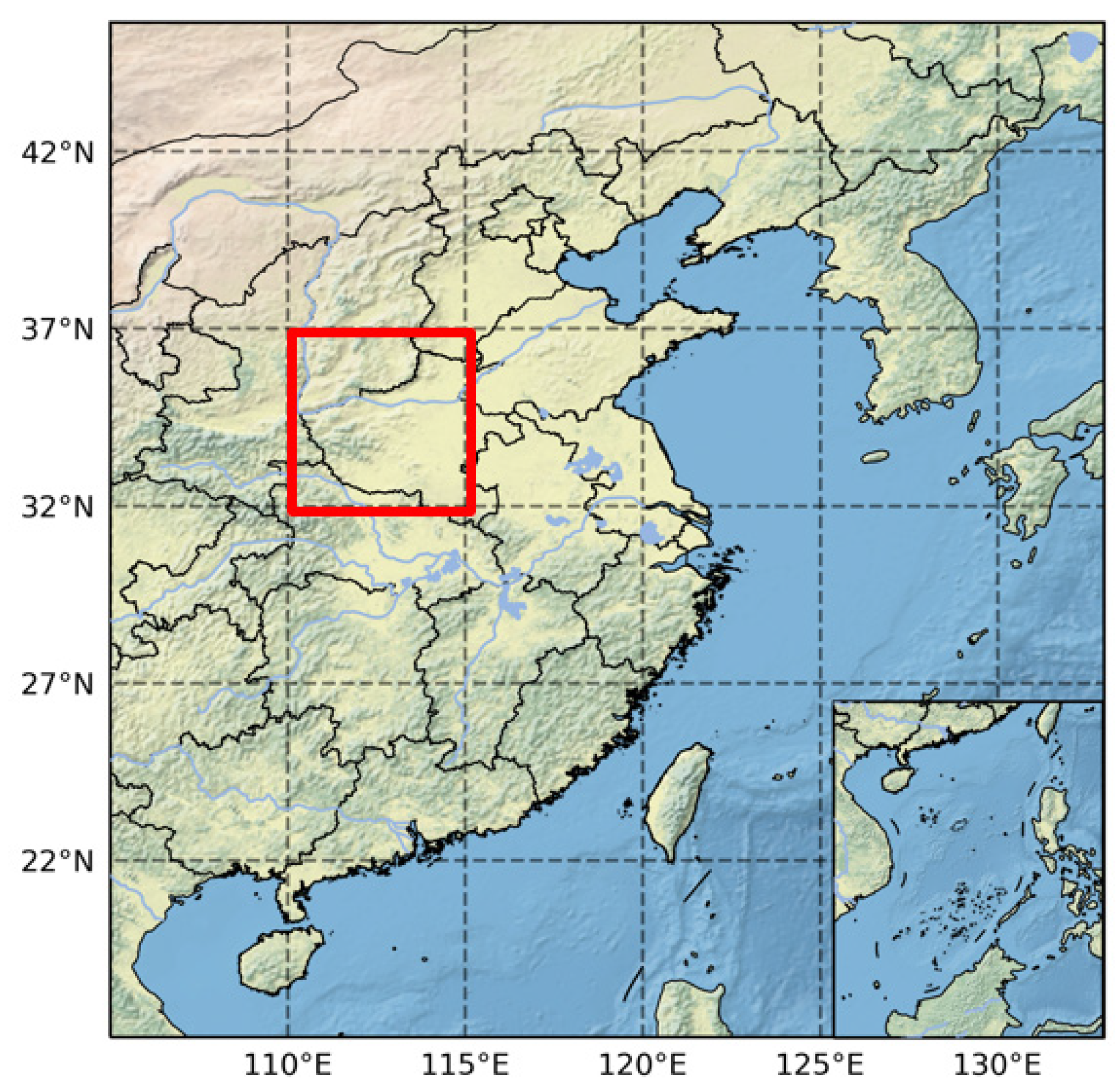
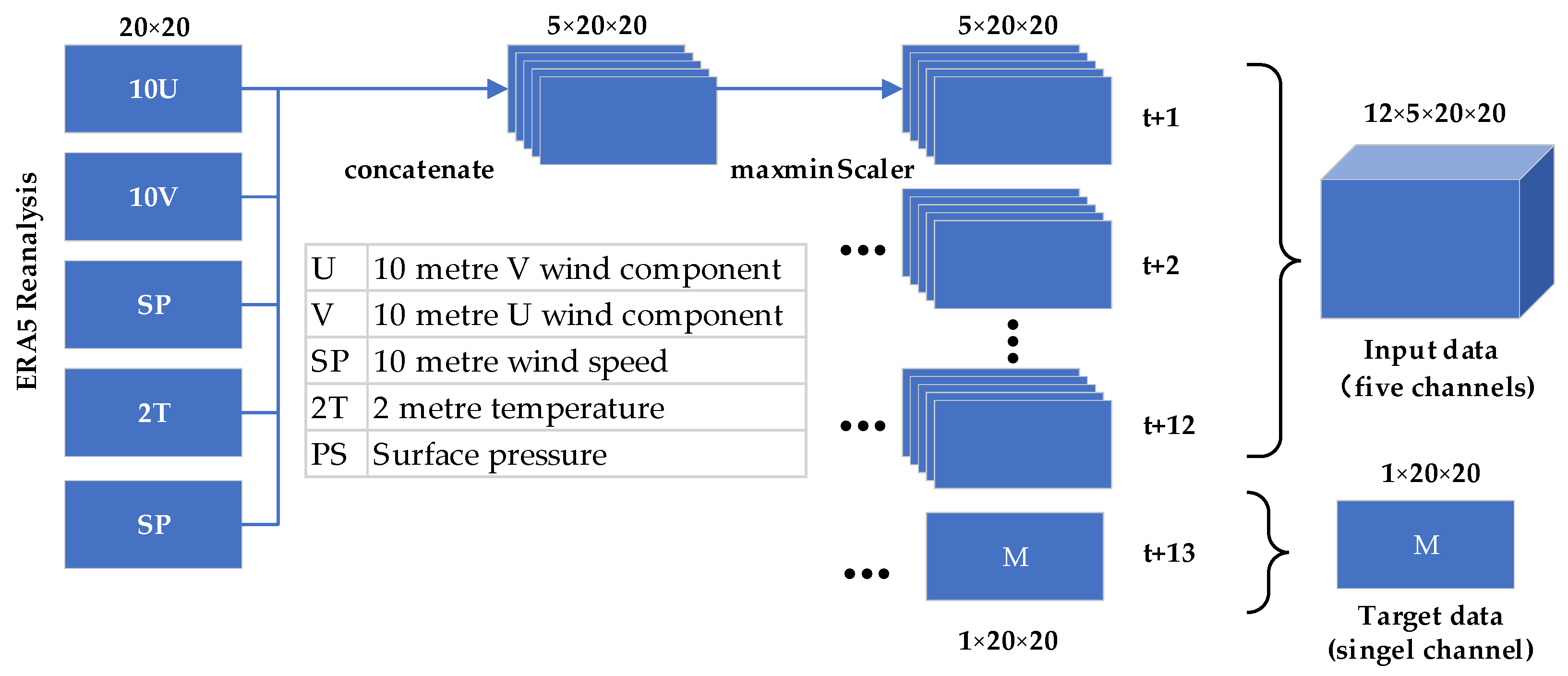
In this study, the ERA5 dataset mentioned above was selected as the model training and testing data. The data area is North China (32–37° N, 110–115° E) and is shown in the red box in Figure 3. In this region, which is located in a plain area, there is abundant wind energy, the wind field turbulence degree is low, and the wind speed and wind direction do not change rapidly due to obstacles or rough wind channels [48,49]. If the wind field turbulence degree is too large, this not only affects the output of the wind turbine, but also makes the wind turbine produce vibration and uneven load, reducing the service life of the wind turbine and, in serious cases, causes the paddle blade to fly out. We selected the data from 2019 to 2021 as the training set and the data from January to February 2022 as the test set. We also collected the data from January to February 2022 from the GRAPES_Meso3km model data as the comparison between the proposed model and the numerical weather-forecasting method for this paper. We selected five channels of data consisting of 2 m temperature, ground-level pressure, 10 m wind U-component, 10 m wind V-component, and 10 m wind speed absolute values. The absolute 10 m wind speed is calculated from the 10 m wind speed U and V components. The 10 m absolute wind speed and 2 m temperature and surface pressure are used as the primary channels, and 10 m wind speed U and V components are used as secondary channels. To reduce the problem of different data magnitudes for different channels, we used the minimum–maximum normalization method to map the dataset to between 0 and 1. We used the 12 previous hourly time steps as model input and the next time step as model output. Since ERA5 is 0.25 degrees and our selected area spans five latitudes and longitudes, we end up with a 20 × 20 grid of data. The data processing flow is shown in Figure 4.

3.4. Experimental Design

To verify the effectiveness of the DACLSTM model proposed in this paper, we chose the ERA5 data from northern China in Section 3.1 for model training and testing, where the data from 2019 to 2021 were used for training and the data from January to February 2022 were used for testing. For model training, we train the model using the normalized training set, and normalization can solve the problem of different units between multiple channels in training. For model prediction, we inverse-normalize the predicted value to calculate the normal wind speed value. We set up two sets of comparison experiments, one of which chooses the ConvLSTM model without the mechanism of adding attention to the work, and the other chooses the fully connected LSTM network model. All experiments were performed with 6-h forecast validity, and our model was designed to input a sequence of 12 h (×1, ×2,…, ×12) and output the next hour (×13), so that only a single moment, i.e., one hour could be forecasted. We used a rolling forecast method, in which the obtained forecast values are appended to the historical data to form a new time series to forecast the next hour.

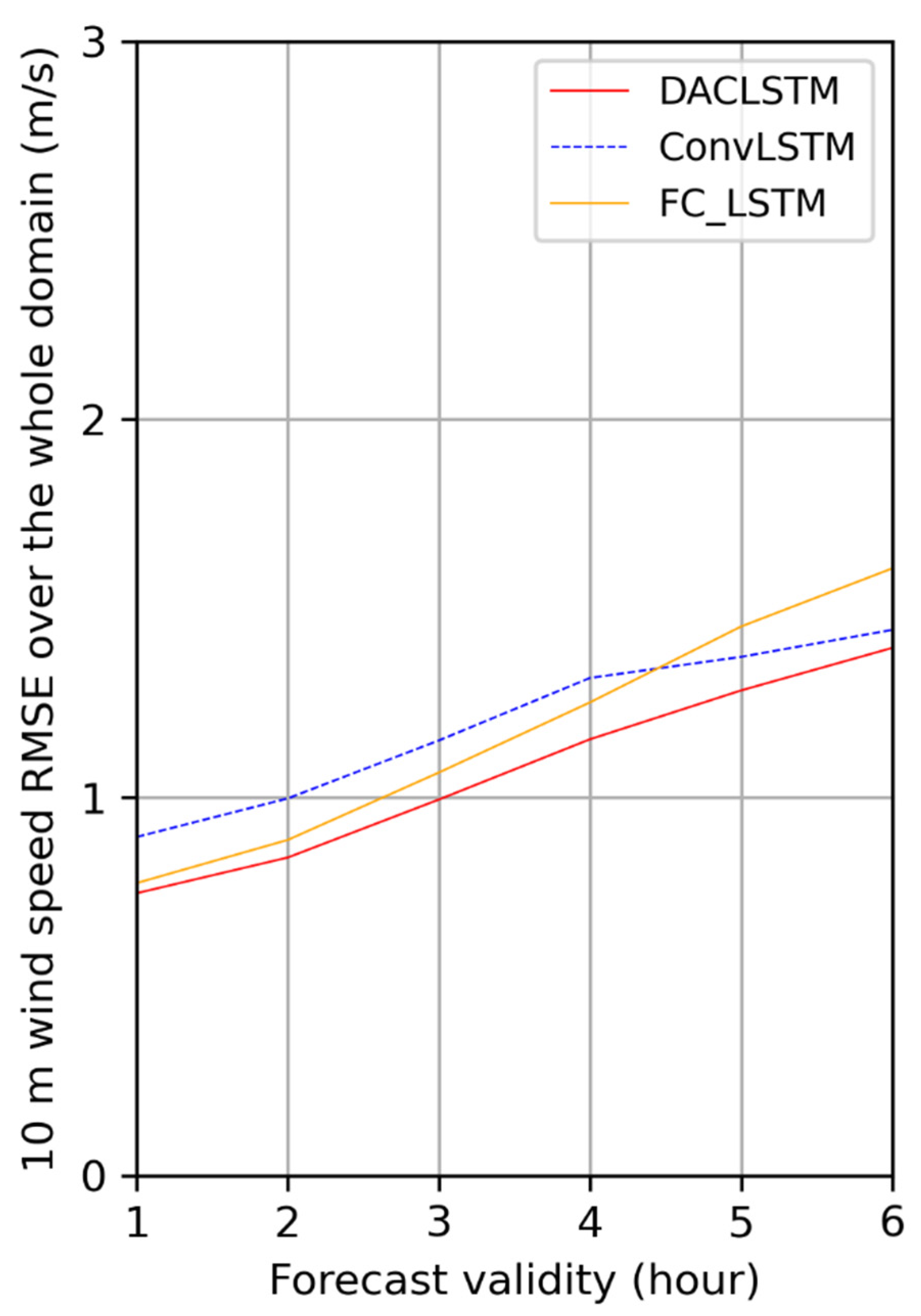
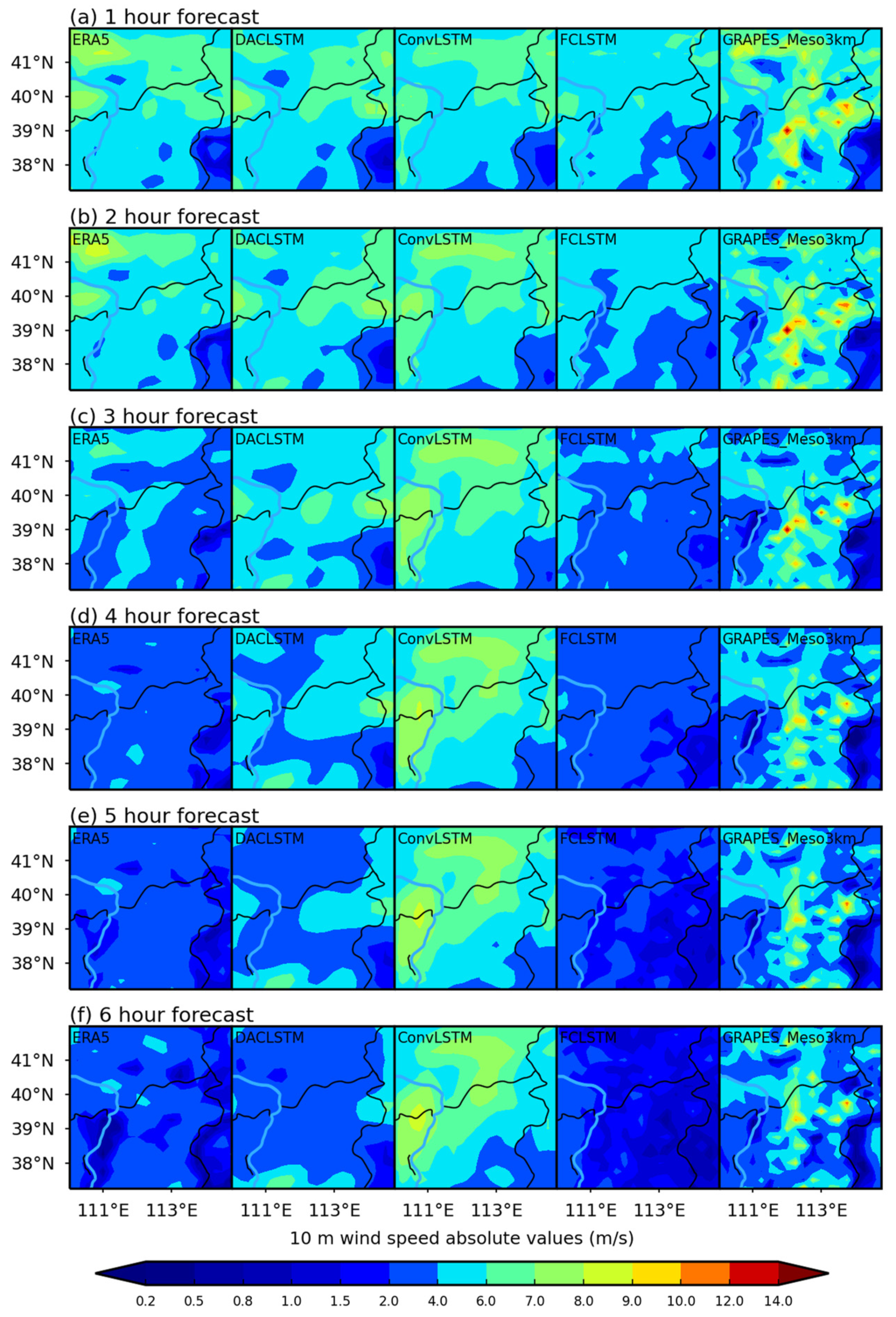
We calculate the RMSE separately for the six-hour-by-six-hour forecasts of the three different models on the test set (January–February 2022). In addition, we calculate hour-by-hour RMSE for different forecast times on the test set for January 2022. In order to compare the forecasting effectiveness of the model proposed in this paper with the GRAPES numerical weather-prediction model, the prediction results of the DACLSTM model were compared with the GRAPES_Meso3km model data in individual cases (on 9 January 2022 at 03:00).

The root mean square error (RMSE) was used for the experimental test index, and we calculated the standard deviation (SD) of the 10 m wind speed in the dataset, the standard deviation of 10 m wind speed in the dataset is 2.3437, and the equations of RMSE and SD are shown below:

$$RMSE=\sqrt{\frac{1}{n}{\displaystyle \sum }_{i=1}^n{\left(t_i-y_i\right)}^2}$$

(8)

$$SD=\sqrt{\frac{1}{n}{\displaystyle \sum }_{i=1}^n{\left(y_i-u\right)}^2}$$

(9)

where n represents the number of samples, t represents the model output value, and y represents the ERA5 actual value, and u represents the average of the data.

4. Results

4.1. Hyperparametric Analiysis

Different hyperparameters have a large impact on model training [50]. Hence, the model parameters proposed in this paper include the maximum number of model iterations, the selection of the activation functions for each layer in each network, and the selection of the model optimizer. The selection of each parameter is specifically analyzed.

We set the value of learning rate as 0.01, use RMSE as the loss function, set the time step to 12 h, and the batch size to 30. After repeated experiments, the maximum number of iterations of the DACLSTM model was determined to be 120. When the number of iterations is less than 120, the model fitting ability is insufficient, i.e., the loss function shows a decreasing trend, as shown in

Table 5. The mean value of loss function under different maximum iterations.

The Mean Value of 3 Experiments
$Ite{r}_{max}$	40	80	120	150
Loss	0.00475	0.003	0.0023	0.0023

. Conversely, when the number of iterations is greater than 120, the value of the loss function remains constant while increasing the training time of the model. It is noted that the smaller the value of the loss function, the better the training effect of the DACLSTM model. Table 5 records the average loss function values for different maximum numbers of iterations for three experiments. Furthermore, the effects of the choice of optimizer and activation function on the mean value of loss are shown in

Table 6. The mean value of loss function under different optimizer and activation functions.

$\mathit{I}\mathit{t}\mathit{e}{\mathit{r}}_{\mathit{m}\mathit{a}\mathit{x}}$	Optimizer	Layer	Activation	Loss
120	Adadelta	ConvLSTM	Tanh	0.0023
		Chanel Attention	Relu + Sigmod
		Spatical Attention	Sigmod
		Dense	Relu
	Adam	ConvLSTM	Tanh	0.0027
		Chanel Attention	Relu + Sigmod
		Spatical Attention	Sigmod
		Dense	Relu
	adagrad	ConvLSTM	Tanh	0.0025
		Chanel Attention	Relu + Sigmod
		Spatical Attention	Sigmod
		Dense	Relu

. The activation functions of each layer were set as Tanh, combination of relu and sigmod, sigmod and relu functions, respectively. The optimizer was set to Adadelta.

4.2. Experimental Results Analysis

From

Table 7. The RMSE of three models for 10 m wind speed forecasting on test dataset (January to February 2022, in North China 32–37° N, 110–115° E) unit (m/s).

Forecast Validity	DACLSTM	ConvLSTM	FC_LSTM
One-hour	0.7464	0.8952	0.7733
Two-hour	0.8408	0.9971	0.8873
Three-hour	0.9941	1.1505	1.0656
Four-hour	1.1535	1.3158	1.2510
Five-hour	1.2827	1.3715	1.4512
Six-hour	1.3951	1.4429	1.6054

and Figure 5, Figure 6, Figure 7, Figure 8, Figure 9, Figure 10, Figure 11 and Figure 12, the following can be seen:

(1)

The performance metrics of the DACLSTM model with the introduction of the dual-attention mechanism outperform the ConvLSTM and FC_LSTM models compared to the traditional single model. For example, in Table 7, the six-hour lead time RMSE of the proposed model’s 10 m wind speed on the test set (January to February 2022) is consistently smaller than that of the ConvLSTM and LSTM; furthermore, Figure 6, Figure 7, Figure 8, Figure 9, Figure 10 and Figure 11 also show that the proposed model has a lower regional average RMSE than the other two models for each hour of 10 m wind speed prediction for different forecast validity.

(2)

The forecasting ability of each model decreases as the forecast time increases, but the DACLSTM model maintains a better forecasting ability. For example, in Figure 12, the DACLSTM model’s 10 m wind speed prediction is most consistent with ERA5 for each forecast period, while the ConvLSTM model and FC_LSTM model move in the other two directions.

(3)

Compared with the GRAPES_3KM numerical forecast of 10 m wind speed, the DACLSTM model can forecast the approximate distribution of wind speed fallout, and the numerical magnitude is also close to that of ERA5. For example, as shown in Figure 12, the 10 m wind speed forecasted by the DACLSTM model can basically agree with ERA5 in 1–2 h, while GRAPES_Meso3K forecasts higher values in the middle compared to the proposed model, which does not agree with ERA5. Within 2–6 h, ERA5 shows uniform wind speeds (2–4 m/s), and the proposed model accurately forecasts the mean value of 10 m wind speed of ERA5, while GRAPES_Meso3km still has higher values in the middle.

5. Conclusions and Discussion

To address the problem of the low accuracy of short-term wind speed forecasting, a ConvLSTM model with a dual-attention mechanism is proposed in this paper. The model was trained using ERA5 one-hour resolution data to achieve wind speed forecasting in the study area and improve the short-term wind speed forecasting capability of the ConvLSTM model. Considering the correlation between wind speed, temperature, and pressure, we first select 2 m temperature, surface pressure, and 10 m wind speed absolute value as the primary channels. The 10 m wind speed absolute value is calculated by 10 m wind speed U-component and V-component. Considering that the 10 m wind speed U and V components directly affect the 10 m wind speed absolute value, we use these two components as secondary channels as well. The dual-attention mechanism of channel attention in the multi-channel model and spatial attention in the two-dimensional data plane was introduced. We used the ConvLSTM method to extract temporal information from spatial information. Previous studies have emphasized the use of spatio-temporal continuity to solve wind speed prediction problems. To further improve the accuracy of wind speed prediction, we introduced a dual-attention algorithm with spatial attention and spatial attention in multiple channels. According to our experimental analysis, the model can predict 10 m wind speed in 1~6 h after introducing the dual-attention and multi-channel mechanisms. By analyzing an individual case of GRAPES_Meso3 km, we found that our proposed model outperforms numerical weather prediction for short-term 10 m wind speed prediction in the selected region and can compensate for the short-term 10 m wind speed prediction of numerical weather prediction to some extent.

The contributions of the model proposed in this paper are as follows: (1) We propose a dual-attention mechanism to improve 10 m wind speed prediction, which can improve 10 m wind speed prediction by focusing on important region information of 10 m wind speed distribution and predicting the approximate distribution of wind speed compared with general machine learning models. (2) The performance of the ConvLSTM model for short-term 10 m wind speed prediction, especially in the first two hours, is improved by introducing a dual-attention mechanism to extract the attention of the data channel and data space in short-term 10 m wind speed prediction. (3) We compared three different forecasting models and found that the combination of attentional mechanism and ConvLSTM model can outperform the single model in short-term 10 m wind speed prediction.

However, there are drawbacks in this paper, which are as follows: (1) The proposed model does not perform as well as expected when forecasting high winds. (2) At present, the experiments have verified the effectiveness in northern China but have not verified the feasibility in other regions. (3) The area selected for the experiment is too small, based on the experimental equipment conditions. The selected data types are small, and the addition of solar radiation, heat flux, and relative humidity data are considered in the future. (4) Since rolling forecasts are used, subsequent forecasts include the errors of the previous forecasts, meaning that the errors accumulate over time, leading to the model’s poor performance in long-term forecasting.

References

1. Tarhan, C.; Çil, M.A. A study on hydrogen, the clean energy of the future: Hydrogen storage methods. J. Energy Storage 2021, 40, 102676. [Google Scholar] [CrossRef]
2. Murshed, M.; Ahmed, Z.; Alam, M.S.; Mahmood, H.; Rehman, A.; Dagar, V. Reinvigorating the role of clean energy transition for achieving a low-carbon economy: Evidence from Bangladesh. Environ. Sci. Pollut. Res. 2021, 28, 67689–67710. [Google Scholar] [CrossRef] [PubMed]
3. Wang, Y.; Zou, R.; Liu, F.; Zhang, L.; Liu, Q. A review of wind speed and wind power forecasting with deep neural networks. Appl. Energy 2021, 304, 117766. [Google Scholar] [CrossRef]
4. Peng, X.; Liu, Z.; Jiang, D. A review of multiphase energy conversion in wind power generation. Renew. Sustain. Energy Rev. 2021, 147, 111172. [Google Scholar] [CrossRef]
5. Fugui, D.; Li, W. Research on the coupling coordination degree of “upstream-midstream-downstream” of China’s wind power industry chain. J. Clean. Prod. 2021, 283, 124633. [Google Scholar]
6. Lei, Y. Studies on wind farm integration into power system. Autom. Electr. Power Syst. 2003, 27, 84–89. [Google Scholar]
7. Zhang, S.; Wei, J.; Chen, X.; Zhao, Y. China in global wind power development: Role, status and impact. Renew. Sustain. Energy Rev. 2020, 127, 109881. [Google Scholar] [CrossRef]
8. Herbert, G.J.; Iniyan, S.; Sreevalsan, E.; Rajapandian, S. A review of wind energy technologies. Renew. Sustain. Energy Rev. 2007, 11, 1117–1145. [Google Scholar] [CrossRef]
9. Yang, X.; Xiao, Y.; Chen, S. Wind speed and generated power forecasting in wind farm. Proc. Chin. Soc. Electr. Eng. 2005, 11, 1–5. [Google Scholar]
10. Bhaskar, K.; Singh, S.N. AWNN-assisted wind power forecasting using feed-forward neural network. IEEE Trans. Sustain. Energy 2012, 3, 306–315. [Google Scholar] [CrossRef]
11. Roungkvist, J.S.; Peter Enevoldsen, P. Timescale classification in wind forecasting: A review of the state-of-the-art. J. Forecast. 2020, 39, 757–768. [Google Scholar] [CrossRef]
12. Zhu, X.; Genton, M.G. Short-term wind speed forecasting for power system operations. Int. Stat. Rev. 2012, 80, 2–23. [Google Scholar] [CrossRef]
13. Nie, Y.; Liang, N.; Wang, J. Ultra-short-term wind-speed bi-forecasting system via artificial intelligence and a double-forecasting scheme. Appl. Energy 2021, 301, 117452. [Google Scholar] [CrossRef]
14. Zhang, Y.; Wang, J.; Wang, X. Review on probabilistic forecasting of wind power generation. Renew. Sustain. Energy Rev. 2014, 32, 255–270. [Google Scholar] [CrossRef]
15. Soman, S.S.; Zareipour, H.; Malik, O.; Mandal, P. A review of wind power and wind speed forecasting methods with different time horizons. In Proceedings of the North American Power Symposium (NAPS) 2010, Arlington, TX, USA, 26–28 September 2010. [Google Scholar]
16. Wu, Y.-K.; Hong, J.-S. A literature review of wind forecasting technology in the world. In Proceedings of the 2007 IEEE Lausanne Power Tech, Lausanne, Switzerland, 1–5 July 2007; pp. 504–509. [Google Scholar]
17. Jung, J.; Broadwater, R.P. Current status and future advances for wind speed and power forecasting. Renew. Sustain. Energy Rev. 2014, 31, 762–777. [Google Scholar] [CrossRef]
18. Ebrahimi, H.; Yazdaninejadi, A.; Golshannavaz, S. Demand response programs in power systems with energy storage system-coordinated wind energy sources: A security-constrained problem. J. Clean. Prod. 2022, 335, 130342. [Google Scholar] [CrossRef]
19. Akhmedovich, M.A.; Fazliddin, A. Current State of Wind Power Industry. Am. J. Eng. Technol. 2020, 2, 32–36. [Google Scholar]
20. Skamarock, W.C. Evaluating mesoscale NWP models using kinetic energy spectra. Mon. Weather. Rev. 2004, 132, 3019–3032. [Google Scholar] [CrossRef]
21. Short, C.J.; Petch, J. Reducing the spin-up of a regional NWP system without data assimilation. Q. J. R. Meteorol. Soc. 2022, 148, 1623–1643. [Google Scholar] [CrossRef]
22. Ulmer, F.-G.; Balss, U. Spin-up time research on the weather research and forecasting model for atmospheric delay mitigations of electromagnetic waves. J. Appl. Remote Sens. 2016, 10, 016027. [Google Scholar] [CrossRef] [Green Version]
23. Jung, T.; Balsamo, G.; Bechtold, P.; Beljaars AC, M.; Koehler, M.; Miller, M.J.; Tompkins, A.M. The ECMWF model climate: Recent progress through improved physical parametrizations. Q. J. R. Meteorol. Soc. 2010, 136, 1145–1160. [Google Scholar] [CrossRef] [Green Version]
24. Durai, V.R.; Bhowmik, S.K.R. Prediction of Indian summer monsoon in short to medium range time scale with high resolution global forecast system (GFS) T574 and T382. Clim. Dyn. 2014, 42, 1527–1551. [Google Scholar] [CrossRef]
25. Chen, D.; Shen, X. Recent Progress on GRAPES Research and Application. J. Appl. Meteorol. Sci. 2006, 17, 773–777. [Google Scholar]
26. Wang, J.; Zhou, Q.; Zhang, X. Wind power forecasting based on time series ARMA model. In IOP Conference Series: Earth and Environmental Science; IOP Publishing: Bristol, UK, 2018; Volume 199. [Google Scholar]
27. Fattah, J.; Ezzine, L.; Aman, Z.; El Moussami, H.; Lachhab, A. Forecasting of demand using ARIMA model. Int. J. Eng. Bus. Manag. 2018, 10, 1847979018808673. [Google Scholar] [CrossRef] [Green Version]
28. Gao, S.; He, Y.; Chen, H. Wind speed forecast for wind farms based on ARMA-ARCH model. In Proceedings of the 2009 International Conference on Sustainable Power Generation and Supply, Nanjing, China, 6–7 April 2009. [Google Scholar]
29. Mitchell, T.M.; Mitchell, T.M. Machine Learning; McGraw-Hill: New York, NY, USA, 1997; Volume 1. [Google Scholar]
30. Guo, Y.; Liu, Y.; Oerlemans, A.; Lao, S.; Wu, S.; Lew, M.S. Deep learning for visual understanding: A review. Neurocomputing 2016, 187, 27–48. [Google Scholar] [CrossRef]
31. Sinha, R.K.; Pandey, R.; Pattnaik, R. Deep learning for computer vision tasks: A review. arXiv 2018, arXiv:1804.03928. [Google Scholar]
32. Voulodimos, A.; Doulamis, N.; Doulamis, A.; Protopapadakis, E. Deep learning for computer vision: A brief review. Comput. Intell. Neurosci. 2018, 2018, 7068349. [Google Scholar] [CrossRef]
33. Sun, Q.D.; Jiao, R.L.; Xia, J.J.; Yan, Z.W.; Li, H.C.; Sun, J.H.; Wang, L.Z.; Liang, Z.M. Adjusting Wind Speed Prediction of Numerical Weather Forecast Model Based on Machine Learning Methods. Meteorol. Mon. 2019, 45, 426–436. [Google Scholar]
34. Shi, X.; Chen, Z.; Wang, H.; Yeung, D.Y.; Wong, W.K.; Woo, W.C. Convolutional LSTM network: A machine learning approach for precipitation nowcasting. Adv. Neural Inf. Process. Syst. 2015, 28, 802–810. [Google Scholar]
35. Burke, A.; Snook, N.; Gagne, D.J., II; McCorkle, S.; McGovern, A. Calibration of machine learning–based probabilistic hail predictions for operational forecasting. Weather. Forecast. 2020, 35, 149–168. [Google Scholar] [CrossRef]
36. Han, N. Machine Learning Correction of Wind, Temperature and Humidity Elements in Beijing-Tianjin-Heibei Region. J. Appl. Meteorol. Sci. 2022, 33, 12. [Google Scholar]
37. Vaswani, A.; Shazeer, N.; Parmar, N.; Uszkoreit, J.; Jones, L.; Gomez, A.N.; Kaiser, Ł.; Polosukhin, I. Attention is all you need. Adv. Neural Inf. Process. Syst. 2017, 30, 6000–6010. [Google Scholar]
38. Liu, Z.; Jiang, P.; Zhang, L.; Niu, X. A combined forecasting model for time series: Application to short-term wind speed forecasting. Appl. Energy 2020, 259, 114137. [Google Scholar] [CrossRef]
39. Chen, G.; Tang, B.; Zeng, X.; Zhou, P.; Kang, P.; Long, H. Short-term wind speed forecasting based on long short-term memory and improved BP neural network. Int. J. Electr. Power Energy Syst. 2022, 134, 107365. [Google Scholar] [CrossRef]
40. Zhang, S.; Zhang, T.; Liu, Y.; Li, W.; Cao, M. A modified framework based on LSTM-FC for wind turbine health status prediction. In Proceedings of the 2020 6th International Conference on Big Data and Information Analytics (BigDIA), Shenzhen, China, 4–6 December 2020. [Google Scholar]
41. Woo, S.; Park, J.; Lee, J.Y.; Kweon, I.S. Cbam: Convolutional block attention module. In Proceedings of the European Conference on Computer Vision (ECCV), Munich, Germany, 8–14 September 2018. [Google Scholar]
42. Wang, F.; Jiang, M.; Qian, C.; Yang, S.; Li, C.; Zhang, H.; Wang, X.; Tang, X. Residual attention network for image classification. In Proceedings of the 2017 IEEE Conference on Computer Vision and Pattern Recognition, Honolulu, HI, USA, 21–26 July 2017. [Google Scholar]
43. Zhang, Y.; Li, K.; Li, K.; Wang, L.; Zhong, B.; Fu, Y. Image super-resolution using very deep residual channel attention networks. In Proceedings of the 2018 European Conference on Computer Vision (ECCV), Munich, Germany, 8–14 September 2018. [Google Scholar]
44. Ye, Q.; Yuan, S.; Kim, T.-K. Spatial attention deep net with partial PSO for hierarchical hybrid hand pose estimation. In European Conference on Computer Vision; Springer: Cham, Switzerland, 2016. [Google Scholar]
45. Hersbach, H.; Bell, B.; Berrisford, P.; Hirahara, S.; Horányi, A.; Muñoz-Sabater, J.; Nicolas, J.; Peubey, C.; Radu, R.; Schepers, D.; et al. The ERA5 global reanalysis. Q. J. R. Meteorol. Soc. 2020, 146, 1999–2049. [Google Scholar] [CrossRef]
46. Bell, B.; Hersbach, H.; Simmons, A.; Berrisford, P.; Dahlgren, P.; Horányi, A.; Muñoz-Sabater, J.; Nicolas, J.; Radu, R.; Schepers, D.; et al. The ERA5 global reanalysis: Preliminary extension to 1950. Q. J. R. Meteorol. Soc. 2021, 147, 4186–4227. [Google Scholar] [CrossRef]
47. Ma, Z.; Han, W.; Zhao, C.; Zhang, X.; Yang, Y.; Wang, H.; Cao, Y.; Li, Z.; Chen, J.; Jiang, Q.; et al. A case study of evaluating the GRAPES_Meso V5. 0 forecasting performance utilizing observations from South China Sea Experiment 2020 of the “Petrel Project”. Atmos. Res. 2022, 280, 106437. [Google Scholar] [CrossRef]
48. Dai, H.; Chen, M.; Wang, W.; Wang, X. The status of wind power development and technical supports in China. Electr. Power 2005, 1, 80–84. [Google Scholar]
49. Zhao, D.Q.; Wang, Y.; Han, X.S. Main Environmental Problem of Wind Electric Power Generation Fiel. Environ. Prot. Sci. 2005, 31, 66–67. [Google Scholar]
50. Kaselimi, M.; Doulamis, N.; Doulamis, A.; Voulodimos, A.; Pro-topapadakis, E. Bayesian-optimized bidirectional LSTM regression model for non-intrusive load monitoring. In Proceedings of the 2019 IEEE International Conference on Acoustics, Speech and Signal Processing (ICASSP), Brighton, UK, 12–17 May 2019. [Google Scholar]
Figure 1. Dual-attention mechanism structure.
Atmosphere 14 00071 g001
Figure 2. Overview of the proposed model.
Atmosphere 14 00071 g002
Figure 3. The selected area in the north of China.
Atmosphere 14 00071 g003
Figure 4. Data pre-processing flow.
Atmosphere 14 00071 g004
Figure 5. 10 m wind speed RMSE over the whole domain with three forecast models in test dataset (January to February 2022, in North China 32–37° N, 110–115° E).
Atmosphere 14 00071 g005
Figure 6. One-hour forecasts of 10 m wind speed RMSE on test dataset (January 2022, in North China 32–37° N, 110–115° E).
Atmosphere 14 00071 g006
Figure 7. Two-hour forecasts of 10 m wind speed RMSE on test dataset (January 2022, in North China 32–37° N, 110–115° E).
Atmosphere 14 00071 g007
Figure 8. Three-hour forecasts of 10 m wind speed RMSE on test dataset (January 2022, in North China 32–37° N, 110–115° E).
Atmosphere 14 00071 g008
Figure 9. Four-hour forecasts of 10 m wind speed RMSE on test dataset (January 2022, in North China 32–37° N, 110–115° E).
Atmosphere 14 00071 g009
Figure 10. Five-hour forecasts of 10 m wind speed RMSE on test dataset (January 2022, in North China 32–37° N, 110–115° E).
Atmosphere 14 00071 g010
Figure 11. Six-hour forecasts of 10 m wind speed RMSE on test dataset (January 2022, in North China 32–37° N, 110–115° E).
Atmosphere 14 00071 g011
Figure 12. Six-hourly forecast 10 m wind speed distribution on 9 January 2022 at 03:00 in North China 32–37° N, 110–115° E.
Atmosphere 14 00071 g012