In-Depth Examination of Machine Learning Models for the Prediction of Ground Temperature at Various Depths

Abstract

Ground temperature (GT) or soil temperature (ST) is simply the measurement of the warmness of the soil. Even though GT plays a meaningful role in agricultural production, the direct method of measuring the GT is time-consuming, expensive, and requires human effort. The foremost objective of this study is to build machine learning (ML) models for hourly GT prediction at different depths (5, 10, 20, and 30 cm) with the optimum hyperparameter tuning with less complexity. The present study utilizes a statistical model (multiple linear regression (MLR)) and four different ML models (support vector regression (SVR), random forest regression (RFR), multi-layered perceptron (MLP), and XGBoost (XGB)) for predicting GT. Overall, 13 independent variables and 5 GTs with different depths as response variables were collected from a meteorological station at an interval of 1 h between 1 January 2017 and 1 July 2021. In addition, two different input datasets named M1 (selected number of parameters) and M2 (collected dataset with all variables) were used to assess the model. The current study employed the Spearman rank correlation coefficient approach to extract the best features and used it as the M1 dataset; in addition, the present study adopted regression imputation for solving the missing data issues. From the results, the XGB model outperformed the other standard ML-based models in any depth GT prediction (MAE = 1.063; RMSE = 1.679; R² = 0.978 for GT; MAE = 0.887; RMSE = 1.263; R² = 0.979 for GT_5; MAE = 0.741; RMSE = 1.025; R² = 0.985 for GT_10; MAE = 0.416; RMSE = 0.551; R² = 0.995 for GT_20; MAE = 0.280; RMSE = 0.367; R² = 0.997 for GT_20). Therefore, the present study developed a simpler, less-complex, faster, and more versatile model to predict the GT at different depths for a short-term prediction with a minimum number of predictor attributes.

1. Introduction

The unabated increase in greenhouse gas emissions is raising the temperature of the Earth. The consequences include melting glaciers, increased precipitation, extreme weather events, and shifting seasons. Combined with global population and income growth, climate change poses a global threat to food security [1,2]. Climate change, in particular, has exacerbated the effects on agriculture in recent decades, owing to changes in the frequency and severity of droughts and floods [2,3]. Climate change will have a wide-ranging impact on the global food equation, both on supply and demand and on food systems at the local level, where small farm communities frequently rely on local and self-production. In addition, it significantly impacts global, regional, and local food production. Climate change is attributed to an increase in greenhouse gases, such as carbon dioxide (CO₂), methane (CH₄), and nitrous oxide (N₂O), and is caused by human activities such as the use of fossil fuels for energy production, agricultural activities, and deforestation. Temperature rise due to global warming is expected to continue, rising from 1.8 °C to 4.0 °C by the end of the century [4]. A recent systematic review of changes in crop yields of major crops grown in Africa and South Asia due to climate change discovered that average crop yields in both regions could fall by 8% by the 2050s [5,6]. Climate change is expected to reduce yields by −17% (wheat), −5% (maize), −15% (sorghum), and −10% (millet) in Africa, and by −16% (maize) and −11% (sorghum) in South Asia [5,6]. The temperature of the Earth’s soil is one of the significant agricultural factors affected by global warming; the characteristics of the Earth’s soil are critical in Earth sciences such as agriculture, forestry, geology, and land-atmosphere interactions [7].

Soil temperature (ST) or ground temperature (GT) is simply the measurement of the warmness of the soil. Soil absorbs and stores heat, acting as an energy driver during the day and a heat source at the soil surface at night. In terms of annual energy transfer, during the warm season, the soil stores energy and releases it into the air during the colder months of the year [8,9]. GT impacts the rate of nitrification; also, it influences the soil moisture content, aeration, and heat energy balance between the atmosphere and land surface. The GT is the factor that drives the germination of seeds; in addition, it directly affects plant growth since GT regulates the soil’s physical and chemical properties. In practice, this soil property can seriously influence nutrient uptake, respiration within the soil’s evaporation and transpiration processes, root and plant growth, and microorganism activity [10,11,12,13]. In contrast, several vital processes, such as dehumidification and the concentration of physical, chemical, and microbiological processes in soil media, are also tremendously governed by the thermos—physical properties of the soil; thereby, knowledge of GT is highly relevant in cultivation-based decision-making tasks. Most soil organisms function best at an optimum soil temperature, which aids in generating quality and an improved production quantity. Metrological variables have an exerted influence on GT; thus, GT and distribution at different depths are manipulated by external climatic factors such as atmospheric air temperature, relative humidity, wind speed, solar radiation, rainfall, atmospherics, and sunshine duration. Furthermore, the soil temperature is an important factor in some other fields, such as water resources and hydrologic engineering. Besides that, in the field of atmospheric science, changes in GT have obvious effects on the decomposition of organic matter, resulting in an increase in carbon dioxide (CO₂) in the atmosphere [14]. As a result, a model which is capable of accurately forecasting GT is in high demand.

Measuring GT only from the surface does not complete the forecasting models because the nature and temperature of the soil vary according to the specific depth. Previous studies have mentioned that a soil depth of 5 cm plays a significant role in seed germination, growth, and nutrient uptake [15]. At a depth of 10 cm, the soil’s nature also governs the growth of microorganisms and their transmission to plants; similarly, the soil at a depth of 20 cm ensures the growth of the roots of plants and the absorption of water and nutrients by the roots [16]. Therefore, predicting GT changes at different depths is indispensable for ensuring the proper growth of plants. There are generally two methods used to measure GT. They are as follows:

(1) Direct measuring method (method of manually inserting high-precision soil temperature sensors into the soil surface and at the required depths).

(2) Indirect method—predictive modeling method (giving atmospheric parameter input to various prediction models and training the models with historical values at the required depths and times).

Even though the direct measuring method is more reliable, such measurements are not only cumbersome but also require a vast number of human resources and an abundance of time. However, the predictive modeling methods are accessible. If the models achieve high accuracy with minimal error in their predictions, they can be used as a navigation for temperature changes. Various kinds of modeling techniques such as statistical modeling, time series modeling, energy balance models, and computational models used for predicting GT have become vastly available in recent years [17,18,19,20]. The following components comprehensively explain modeling concepts and methods.

Statistical and time series-based models are established through the relationship between GT and climatological variables. The previous statistical model which was used for GT prediction correlates the interrelationship between air temperature, relative humidity, wind speed, solar radiation, rainfall, atmospherics, and sunshine duration and the GT [17,18,19,20,21,22,23,24]. Even though most statistical models adopt linearity between the independent and dependent variables, the GT is nonlinear to the other climatological variables, so such models are not optimal for predicting future GT. Other widely used models are time series-based models known as Box–Jenkins models for GT, which work by predicting future values from past historical time-based values. Among the other time series-based statistical models, the auto-regressive moving average (ARMA) model and the auto-regressive integrated moving average (ARIMA) model are extensively used for future prediction [25,26,27]. Previous studies’ [26,28] results show that the temperature series is not sufficiently static for these models. So, the reliability of these models is still a question for various depth predictions.

Machine learning (ML), a subcategory of artificial intelligence (AI), has been comprehensively employed to solve nonlinear problems for the last two decades. To solve the GT prediction scenario, several researchers have used neural network-based frameworks. Unlike physical models, ML models adopt the trends of input and output parameters through their self-learning competence. Artificial neural network (ANN), classification and regression trees (CART), random forest regression (RFR), support vector regression (SVR), multiple linear regression modeling, boosted regression tree (BRT), long short-term memory network (LSTM), gated recurrent unit network (GRU), etc., are some models often used not only used for GT prediction but also for rainfall-runoff, climate prediction, and indoor microclimates [1,11,29,30]. In a previous study, Ref. [19] utilized an ANN model to estimate daily and annual GT, and the results showed that the ANN model could sufficiently predict the GT. Likewise, another study [10] developed an ANN model used to predict monthly soil temperature by using various meteorological variables of the previous month for the city of Adana, Turkey. That study used seven atmospheric variables to predict the GT at various depths by using the three-layered feed-forward-based ANN structure and network to predict the GT with satisfactory results. Later, Ref. [31] conducted a comparative study between ANN, an adaptive neuro-fuzzy inference system (ANFIS), and gene expression programming (GEP) for predicting GT at four different depths (5, 10, 50, and 100 cm) at 31 studied stations in Iran. In this process, the geographical information (latitude, longitude, and altitude) and periodicity component (the number of months) were applied as inputs in the used models. The results showed that the utilization of the ANFIS model enhanced the prediction accuracy of the soil temperature for all 31 stations. After the evolution of the vast number of machine learning algorithms, several studies used SVR, RFR, and other machine-learning models such as genetic algorithm (GA) and a gradient-boosting decision tree (GBDT) for predicting the GT.

Recently, deep learning- (DL) based recurrent neural network (RNN) models were used to predict short- and long-term data. For instance, Ref. [32] employed an autoregressive integrated moving average (FARIMA) model to predict the GT, and the model’s performance compared with gene expression programming (GEP) FFBPNN. The results indicate FARIMA outperformed the FFBPNN and GEP methods in terms of prediction accuracy; however, FARIMA’s predictions are relatively inadequate for acute GT values. Previous literature [33] utilized RNN-DL-based LSTM, GRU, ANN, and extreme learning machine models (ELM) to predict GT at 5, 10, and 15 cm depths. The results show that the model predictions are not significantly different between the RNN models. Even though the DL-RNN-based models still produce better prediction, there is some limitation with the time series-based RNN models acclaimed from the previous studies [14,33,34]. Those limitations are (1) that the time series-based RNN models struggle to predict the missing information over a long time series, and (2) that these kinds of time series models are good enough to produce more accuracy in long-time predictions with more significant historical inputs, but are flawed in the case of short-time predictions with fewer data. Such limitations mentioned above have led the researchers adopt simple ML models to predict the GT at different depths in the short term.

Since there is a knowledge gap in utilizing ML models for predicting GT at different depths, the current study is intended to build an optimal model with less complexity in short-term prediction. The present study utilizes a statistical model (multiple linear regression (MLR)) and four different ML models (SVR, RFR, MLP, and XGBoost (XGB)) for predicting GT. In addition, numerous metrological parameters are available from the weather stations. The use of more input parameters increases the complexity of the model. Using the proper input parameters creates room to learn more quickly and accurately about the models. Unlike statistical models, selecting the suitable parameter and inputting it into the ML models increases accuracy and training time. The primary objectives of this study are as follows:

(1) Building ML learning models for hourly GT prediction at different depths (5 cm, 10 cm, 20 cm, and 30 cm) with the optimum hyperparameter tuning with less complexity.

(2) Comparing the accuracy of all the models using two different datasets: (1) selected number of parameters and (2) collected dataset with all variables.

(3) Comparing the statistical and ML model performance for the prediction of GT.

2. Materials and Methods

2.1. Site Description and Data Collection

The current study examines the GT of Busan, South Korea’s second-most populous metropolitan city after Seoul, with over 3.4 million inhabitants. South Korea is in the temperate climate zone of the mid-latitude (34–43° N) geographical area, with distinct seasons of spring, summer, autumn, and winter. The metrological data were collected from the Busan metrological station (35°06′19.0″ N, 129°01′55.8″ E). Busan’s daily mean temperature is 15.0 °C, average high temperature is 19.2 °C, average low temperature is 11.7 °C, average relative humidity is 63.3%, and average precipitation is 1576.7 mm as recorded from the last 30 years’ metrological data. The data collected from 1 January 2017 to 1 July 2021 (4.7 years) were used for modeling and validation. Because climate change has recently had a significant impact on agriculture, recent data with short intervals were chosen for the current study. Overall, 13 independent variables and 5 GTs with different depths (GT, GT_5, GT_10, GT_20, and GT_30) as response variables were collected at an interval of 1 h. Figure 1 depicts the location of the Busan metrological station, and

Table 1. Statistical summary of the GT associated parameters.

S.No	Variable Name	Nomenclature	Unit	Skewness	Kurtosis	Mean	SD	Min	Max
1	Temperature	Te	(°C)	−0.25	−0.64	15.04	8.42	−12.2	36.1
2	Precipitation	Pr	(mm)	21.27	708.72	2.03	1.47	0	78.8
3	Wind speed	WS	(m/s)	1.09	2.59	3.16	1.76	0	18.1
4	Wind direction	WD	(Azimuth)	−0.04	−1.41	181.44	111.16	0	360
5	Humidity	Hu	(%)	−0.15	−0.85	62.29	20.87	7	100
6	Vapor pressure	VP	(hPa)	0.59	−0.75	12.9	8.6	0.6	36.3
7	Dew point temperature	DT	(°C)	−0.42	−0.66	7.15	11.68	−29	27.3
8	Local atmospheric pressure	AP	(hPa)	−0.18	−0.05	1007.5	7.41	952.2	1027.1
9	Barometric pressure	BP	(hPa)	−0.16	−0.12	1015.8	7.66	959.7	1036
10	Sunshine	SS	(h)	−0.27	−0.8	0.55	0.33	0	1
11	Solar radiation	SR	(MJ/m2)	0.83	1.25	1.17	0.74	0	4.77
12	Mid-lower cloud cover	Cl	(decile)	0.78	−1.05	2.82	3.54	0	10
13	Visibility	Vi	(10 m)	1.37	1.62	2019.5	1178	14	5000
14	Ground temperature	GT	(°C)	0.44	0.29	17.18	11.68	−10	66.3
15	5 cm underground temperature	GT_5	(°C)	0.1	−0.84	16.78	8.97	−4.4	44.7
16	10 cm underground temperature	GT_10	(°C)	0.04	−1.03	16.61	8.43	−0.5	40.7
17	20 cm underground temperature	GT_20	(°C)	0.02	−1.16	16.72	7.84	1.5	35.4
18	30 cm underground temperature	GT_30	(°C)	0.02	−1.21	16.68	7.46	2.4	32.6

depicts the collected parameters with a basic description.

2.2. Used Data

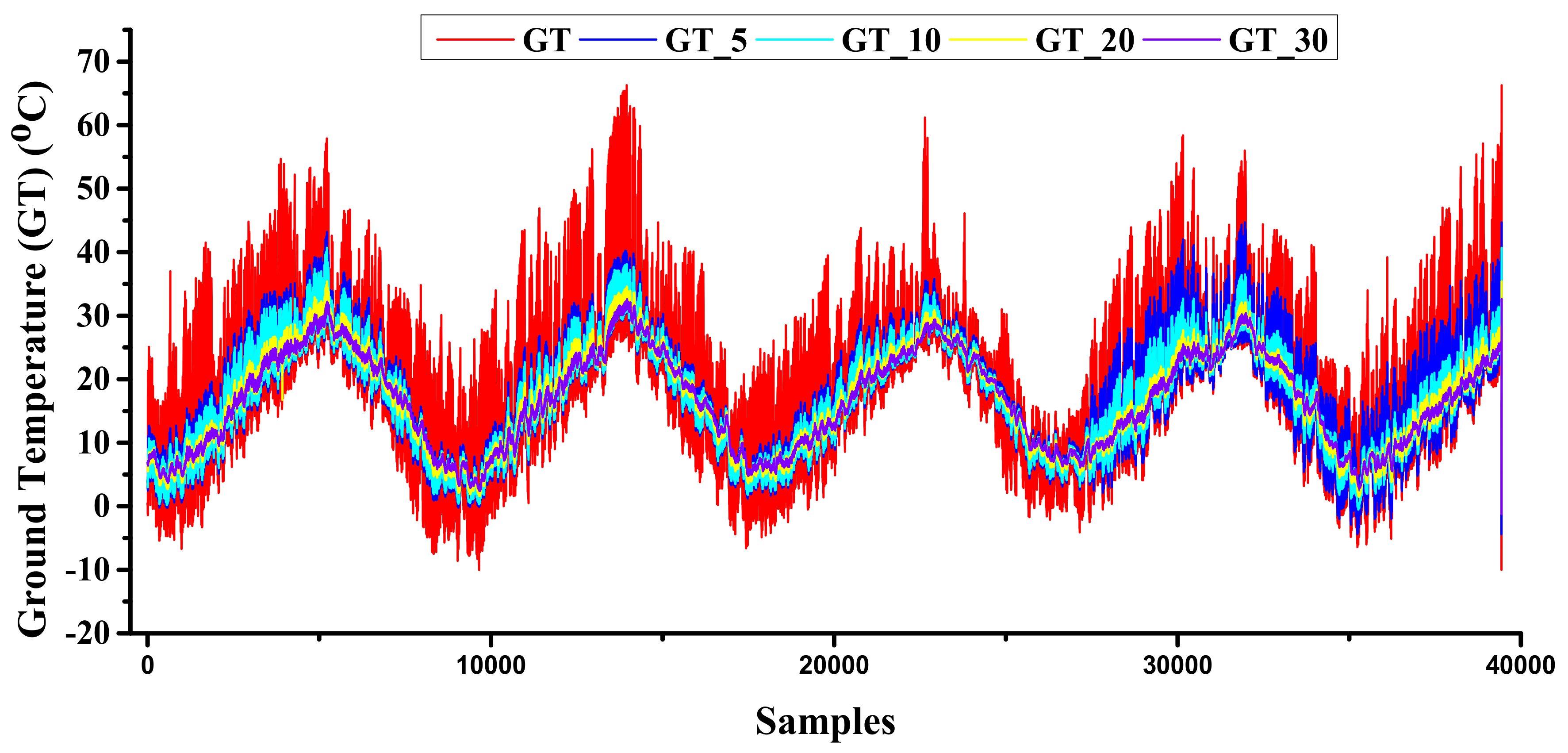
As mentioned above, a dataset consisting of 13 independent variables and 5 dependent variables was collected from the metrological stations. Since it is an open dataset, missing values should also be considered before using the data for training/testing. In order to avoid such issues, exploratory data analysis (EDA) procedures were followed [10,11,29]. EDA is an approach to summarize the data by taking their main characteristics and visualizing them with proper representations. EDA focuses more narrowly on checking assumptions required for model fitting and hypothesis testing, and handling missing values and making transformations of variables as needed [35]. Later, the method of cleaning the missing values is described in this study. The basic description of the dataset is shown in Table 1 in a detailed manner with mean, standard deviation, minimum, maximum, kurtosis, and skewness known through the basic interpretation of the data. Figure 2 explains the graphical description of the GT using data from various depths.

As mentioned in the objective for this study, two different datasets were used for training/testing the model. To achieve the desired accuracy with less computational cost, a reference for selecting the parameters to be recorded must be generated. Selecting an appropriate input source is a key in the ML technique to obtain superlative productivity from the algorithms [1,11]. As a result, the current study employs the Spearman rank correlation coefficient approach to extract the best features, a widely used method for investigating relationships between attributes. The heat correlation map using the Spearman rank correlation coefficient for the GT, GT_5, GT_10, GT_20, and GT_30 is shown in Figure 3. According to the correlation map, highly correlated variables have been selected for the first dataset, so that the current study used two datasets for GT-modeling purposes, named M1 (“Te, VP, DT, AP, BR, and SR” as the independent variables) and M2 (collected all independent variables).

2.3. Model Development

2.3.1. Multiple Linear Regression

Multiple linear regression (MLR) is a more extended version of simple linear regression (SLR). It is popular among other statistical models because of its candid nature, calculation interpretability, and understanding of outlines or anomalies within the dependent variables [36,37]. These models are widely used in various fields, including business foresting, power consumption, energy consumption prediction, weather forecasting, and so on. MLR models make the following assumptions:

MLR can be mathematically expressed by the following formula [36,37]:

$${\mathrm{Y}=\mathrm{a}}_0{+\mathrm{a}}_1{\mathrm{X}}_1{+\mathrm{a}}_2{\mathrm{X}}_2{+\dots +\mathrm{a}}_{\mathrm{i}}{\mathrm{X}}_{\mathrm{i}}+\mathsf{\epsilon }$$

(1)

where Y is the dependent variable; a₀ is the intercept or constant of the model; X₁, X₂, …, X_i are the independent variables; a₁, a₂, …, a_i are the regression coefficients; and the ε is the noise or random error of the model.

2.3.2. Multi-Layered Perceptron

The multi-layer perceptron (MLP) is a fundamental, classical type of neural network model for overcoming linear models, because linear models can extract attributes’ relationships [10]. MLP models have been developed to solve nonlinearity problems by combining back-propagation (BP) techniques with perceptron. Because the MLP has a three-layer structure (an input layer, a hidden layer, and an output layer), weights have been generated for each layer. The weights are updated until the optimal results are given to the output layer, which is the main advantage of BP techniques [38,39]. Finally, the weighted sum of the input layer is converted as output using a nonlinear activation function. This procedure entails lowering the output layer’s prediction error. The neural network technique is essential for data classification and regression because it can adapt and adjust to the data regardless of the primary mode’s special functional or distributional requirements. The MLP with BP can be expressed as follows [38,39]:

$${\mathrm{y}}_{\mathrm{p}}{=\mathrm{f}}_0\left[{\displaystyle \sum }_{\mathrm{j}=1}^{\mathrm{n}}{\mathrm{w}}_{\mathrm{kj}}{\mathrm{f}}_{\mathrm{h}}\left({\displaystyle \sum }_{\mathrm{j}=1}^{\mathrm{m}}{\mathrm{w}}_{\mathrm{ji}}{\mathrm{x}}_{\mathrm{i}}{+\mathrm{w}}_{\mathrm{jb}}\right){+\mathrm{w}}_{\mathrm{kb}}\right]$$

(2)

where y_p is the output (predicted); n is the number of output neurons; f₀ is the activation function for the output neuron; w_kj is the connecting neuron of the hidden and output layers’ weight; f_h is the activation function of the hidden neuron; m is the number of hidden neurons; w_ji is the weight for the connecting neuron of input and hidden layers; x_i is the input variable; w_jb is the bias for the hidden neuron; and w_kb is the bias for the output neuron.

As mentioned earlier, during BP training, the bias and weights were generated until the threshold levels were reached. Such threshold-level training methods reduce the evaluation metrics of the predicted values. So, the updated weight can be expressed as [38,39]

$${\mathrm{W}}_{\mathrm{X}}^{*}{=\mathrm{W}}_{\mathrm{X}}-\mathrm{a}(\frac{{\partial }_{\mathrm{Error}}}{\partial {\mathrm{W}}_{\mathrm{X}}})$$

(3)

where W_X* is the updated weight, W_X is the old weight, a is learning rate, and ∂_Error is the derivative of error with respect to the weight.

The threshold method to stop the training used in this study is root means square error (RMSE), which is also called an error function. According to the model, training should be stopped if minimum RMSE is found during the training time. That error function can be expressed as

$$\mathrm{E}={\displaystyle \sum }_{\mathrm{p}=1}^{\mathrm{p}}{\mathrm{E}}_{\mathrm{p}}={\displaystyle \sum }_{\mathrm{p}=1}^{\mathrm{p}}.{\displaystyle \sum }_{\mathrm{k}-1}^{\mathrm{n}}{\left({\mathrm{y}}_{\mathrm{p}}-{\mathrm{y}}_{\mathrm{a}}\right)}^2$$

(4)

where E is the error of the input patterns and E_p is the square difference between the actual value and predicted value. $\mathrm{Y}$_a is the actual observed data, whereas $\mathrm{y}$_p is predicted data.

2.3.3. Random Forest Regression

Random forest regression is a supervised learning algorithm that performs regression using the ensemble learning method. A technique that combines predictions from multiple machine-learning algorithms to make a more accurate prediction than a single model is known as ensemble learning [1,30]. Similarly, RFR is an ensemble learning technique that consists of aggregating multiple decision trees (DT), resulting in a lower variance compared to single decision trees. The out-of-bags (OOB) error is used to estimate the generalization error of RFR for training points that are not contained in the bootstrap training sets (about one-third of the points are left out in each bootstrap training set). Because OOB is indistinguishable from N-fold cross-validation, the process of OOB estimation is responsible for its non-overfitting nature. Random forest is based on the bagging technique, which aids in the optimization of the algorithm’s performance. It performs well “out-of-the-box,” requiring no hyperparameter tuning, and outperforms linear algorithms, making it a viable option [40,41,42]. Furthermore, random forest is relatively fast and robust, and it can display feature importance, which can be quite useful. The expression of RFR can be represented as following equation [40,41,42]:

$$\mathrm{Y}=\frac{1}{\mathrm{M}}{\displaystyle \sum }_{\mathrm{i}=1}^{\mathrm{M}}\mathrm{H}\left({\mathrm{T}}_{\mathrm{i}}\right) \mathrm{where} \mathrm{H}\left({\mathrm{T}}_{\mathrm{i}}\right) \mathrm{from} \mathrm{DTR}$$

(5)

where M is the total trees; Y is the final output; H (T_i) is a sample in the training set; and T_i is the one sample among all the n subsets which encompasses the total amount of training data.

2.3.4. Support Vector Regression

Vapnik proposed support vector regression (SVR) as a subset of support vector machines (SVMs) in 1992 [43,44]. Because SVMs are statistical, root-based algorithms, they were initially used only to solve classification-related problems. The general concept behind SVMs is to map the original data, X, into a high-dimensional feature space, F, using a nonlinear mapping function and then build an optimal hyperplane in the new space. During that time, SVMs had some important hyperparameters such as kernel (which aids in the discovery of a hyperplane in higher dimensional space), hyperplane (the middle line that separates the classes), and a decision boundary (minimum and maximum boundary lines). SVR was later developed as a regression-solver by Drucker and Vapnik in 1996 using the same concept as SVMs [43,44]. The structural risk minimization (SRM) principle is used to train the SVR, which uses a hypothesis space of linear functions in a high-dimensional feature space. A nonlinear mapping function maps the SVR input into a high-dimensional feature space. That is why SVR is so popular among ML models for solving regression problems. If y is the output variable, then the SVR prediction process can be expressed as follows [44,45,46]:

$$\mathrm{y}=\mathrm{f}\left(\mathrm{x}\right)=\mathsf{\omega }.\mathsf{\phi }\left(\mathrm{x}\right)+\mathrm{b}$$

(6)

where x is the input of the datasets; ω and b are the parameter vectors; and φ(x) is the mapping function assumed by the SVR. Here, y can have unlimited prediction possibilities if it has a multidimensional dataset. So, a limitation for the constraints proposed to determine the optimization issues [44,45,46] could be expressed as

$$\begin{gathered} \mathrm{Minimize}: \frac{1}{2} \left|\left|{\mathsf{\omega }}^2\right|\right|+\mathrm{C}{\displaystyle \sum }_{\mathrm{i}=1}^{\mathrm{n}}\left({\mathsf{\xi }}_{\mathrm{i}}+{\mathsf{\xi }}_{\mathrm{i}}^{*}\right) \\ \mathrm{Subject} \mathrm{to} \left\{\begin{array}{c}{\mathrm{y}}_{\mathrm{i}}-\left(\mathsf{\omega }.\mathsf{\phi }\left(\mathrm{x}\right)+\mathrm{b}\right) \le \mathsf{\epsilon }{+\mathsf{\xi }}_{\mathrm{i}}\\ \left(\mathsf{\omega }.\mathsf{\phi }\left(\mathrm{x}\right)+\mathrm{b}\right)-{\mathrm{y}}_{\mathrm{i}} \le \mathsf{\epsilon }{+\mathsf{\xi }}_{\mathrm{i}}^{*}\\ {\mathsf{\xi }}_{\mathrm{i}}{,\mathsf{\xi }}_{\mathrm{i}}^{*} \ge 0, \mathrm{i}=1,\dots ,\mathrm{n}\end{array}\right. \end{gathered}$$

(7)

where ε is the minimum and maximum margin line/sensitivity zone of the hyperplane; ξ and ξ_i* are the slack variables that measure the training errors which are subjected to ε; and C is the positive constant. To minimize the error between the sensitive zones of the hyperplane, the slack variables were utilized. The sensitive zones can also be expressed using Lagrange multipliers, and the optimization techniques to solve the dual nonlinear problem can be rewritten as the following equation [44,45,46]:

$$\begin{gathered} \min : \frac{1}{2} {\displaystyle \sum }_{\mathrm{i}=1}^{\mathrm{n}}{\displaystyle \sum }_{\mathrm{j}=1}^{\mathrm{n}}\left({\mathrm{a}}_{\mathrm{i}}-{\mathrm{a}}_{\mathrm{i}}^{*}\right)\left({\mathrm{a}}_{\mathrm{j}}-{\mathrm{a}}_{\mathrm{j}}^{*}\right)\mathrm{K}+\mathsf{\epsilon }{\displaystyle \sum }_{\mathrm{i}=1}^{\mathrm{n}}\left({\mathrm{a}}_{\mathrm{i}}{+\mathrm{a}}_{\mathrm{i}}^{*}\right)-{\displaystyle \sum }_{\mathrm{i}=1}^{\mathrm{n}}{\mathrm{y}}_{\mathrm{i}}\left({\mathrm{a}}_{\mathrm{i} }-{ \mathrm{a}}_{\mathrm{i}}^{*}\right) \\ \mathrm{Subject} \mathrm{to} \left\{\begin{array}{c}{\displaystyle {\displaystyle \sum }_{\mathrm{i}=1}^{\mathrm{n}}}\left({\mathrm{a}}_{\mathrm{i}}-{\mathrm{a}}_{\mathrm{i}}^{*}\right)=0\\ 0 \le { \mathrm{a}}_{\mathrm{i}}{, \mathrm{a}}_{\mathrm{i}}^{* }\le \mathrm{C}, \mathrm{i}=1,\dots , \mathrm{n}\end{array}\right. \end{gathered}$$

(8)

where a_i and a_i* are the Lagrange multipliers which are subject to ε, and K is the kernel function. The kernel function uses the kernel trick to solve nonlinear problems using a linear classifier. Generally, linear, radial basis function (RBF), polynomial, and sigmoid are the used kernel functions of SVR models [44,45,46]. The current study chose RBF as the kernel function to optimize SVR during simulation after a random test of other kernel functions. The RBF kernel function can be expressed as the following equation:

$$\mathrm{K}\left(\mathrm{I},\mathrm{j}\right)=\exp (-\mathsf{\gamma }{\left|{\mathrm{x}}_{\mathrm{i}}-{\mathrm{x}}_{\mathrm{j}}\right|}^2)$$

(9)

where, γ is referred to as the structural parameter of the RBF kernel function. Finally, the decision function of SVR can be expressed as [45,46]

$$\mathrm{f}\left({\mathrm{x}}_{\mathrm{i}}\right)={\displaystyle \sum }_{\mathrm{i}=1}^{\mathrm{n}}\left({\mathrm{a}}_{\mathrm{i}}-{\mathrm{a}}_{\mathrm{i}}^{*}\right)\mathrm{K}\left({\mathrm{x}}_{\mathrm{i}}{,\mathrm{x}}_{\mathrm{k}}\right)+\mathrm{b}$$

(10)

2.3.5. Extreme Gradient Boosting

Extreme gradient boosting (XGBoost) is a kind of boosting algorithm proposed by Chen and Guestrin in 2011 and later optimized by several researchers [47,48,49]. XGBoost functions based on boosting-tree algorithms. Unlike the DT, RFR, and other boosting-tree-based algorithms, XGB combines the results of the weak learner group and the strong learner group, then produces cumulative results. Only the first derivative information is used in traditional boosting-tree models. It is difficult to implement distributed training when training the nth tree because the residual of the previous n − 1 trees is used. XGBoost performs a second-order Taylor expansion on the loss function and automatically uses the CPU’s multithreading for parallel computing [48,49]. First, the initial learner is fitted to the interior environment of input data. The second model is then fitted with the residual of the first learner in order to improve the previous learner’s weak learning ability. Until the threshold is satisfied, the accumulation process is repeated. The algorithm’s final predictive result is calculated by adding the predictions of all learners. Since XGB algorithms use optimized resources and optimal speed calculation through parallel computing ability, they are fast learners and successors of boosting-family accuracy. As mentioned above, the first step of prediction is expressed as follows [40,47,48,49]:

$$f_i^{\left(t\right)}={\displaystyle \sum }_{k=1}^t{f}_k\left(x_i\right)=f_i^{\left(t-1\right)}+f_i\left(x_i\right)$$

(11)

where $f_i\left(x_i\right)$ is the learner in step t, $f_i^{\left(t\right)}$ and $f_i^{\left(t-1\right)}$ are the predicted values in steps t and t − 1, and $x_i$ is the input observation. In order to prevent the over-fitting of the training data from affecting the calculation speed of the model, the XGB model uses the following equation to evaluate the model [40,47,48]:

$$Ob{j}^t={\displaystyle \sum }_{k=1}^{n}l\left(y_i^{-}, y_i\right)+{\displaystyle \sum }_{k=1}^t\mathsf{\Omega }\left(f_i\right)$$

(12)

where l represents the loss function, n represents the amount of input data, and Ω represents the regular term, which is defined as follows [40,47,48]:

$$\mathsf{\Omega }\left(f\right)=\gamma T+\frac{1}{2}\lambda {||\omega ||}^2$$

(13)

where ω represents the leaf score, λ is the hyperparameter of the regular term, and γ represents the minimum loss that the leaf node needs to split.

2.4. Modeling Concept

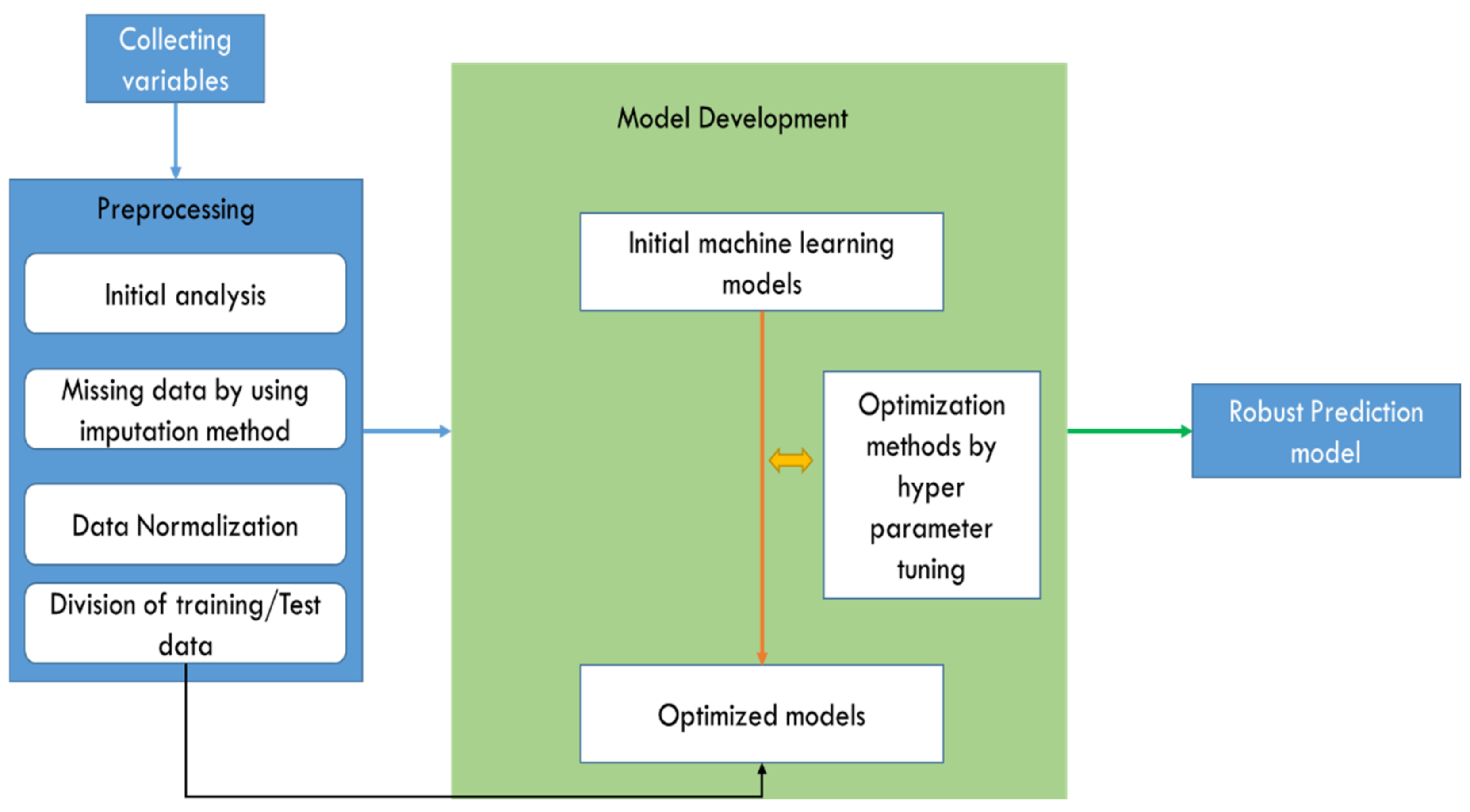
The current part explains the thought framework of the current study; the graphical representation of the study is shown in Figure 3 as a step-by-step flow chart. Firstly, the metrological data for every 1 h was collected and stored. Overall, 18 variables, including the dependent variables, were stored and underwent preprocessing/EDA analysis. As the next step, the missing data for every attribute were checked. In general, missing data are highly disputed for most ML modeling fields in metrological studies [50,51,52]. Various researchers have already conducted work on solving the missing data. Most of the studies remove the missing data and model their datasets; such models are not reliable enough when it comes to modeling. Some statistical theories, such as linear interpolation, data imputation, the k-nearest neighbor algorithm, etc., are available to resolve the missing data dispute [50,51,52].

The current study adopts regression imputation, which is familiar and more competent for solving the missing data dispute. Regression imputation is similar to single linear regression, but can also be used for the multiple missing variables. If data are missing at random (MAR), regression imputation, also known as conditional mean imputation, replaces each missing value with a predicted value based on a regression model [50]. A general regression procedure is divided into two stages: first, a regression model is constructed using all of the available complete observations, and then missing values are estimated using the constructed regression models. The current study uses the “sklearn” (python-based library) to impute the missing data. Both independent data and dependent data are imputed separately in order to avoid the pre-training errors. Next, the distribution of every attribute is considered through skewness and kurtosis. As mentioned earlier, since the current study intends to state and art of the ML model’s performance, the Spearman rank correlation test was examined to choose the best features. The heat correlation map of every response variable is shown in Figure 4 and Figure 5.

The next step of preprocessing is the normalization of the data considered. Data normalization is a standard procedure if attributes are in different ranges. A different range of variables complicates the learning of any ML algorithm [1,11,37]. In order to achieve better efficiency and higher accuracy, mapping the data to a specific range will avoid the consequences aforementioned. Minimum-maximum (min-max) normalization is a common normalization technique used in machine learning which may rescale the variables from the range of −1 to 1 or 0 to 1. The current study employed a min-max scalar with the range of −1 (minimum) to 1 (maximum) to rescaling; this could be mathematically expressed by [1,11,37]

$${\mathrm{x}}_{\mathrm{nor}}=\frac{{2\ast (\mathrm{x} - \mathrm{x}}_{\min })}{{(\mathrm{x}}_{\max }-{\mathrm{x}}_{\min })}-1$$

(14)

where x_nor is the normalized data, X_max is the maximum of original data, x_min is the minimum of original data, and x is the original data. Next, training and testing data were partitioned to feed the training data for the ML algorithms. Still, there is no proper definition for the splitting of training and testing data. Most often, three ratios are commonly followed by ML practitioners: 70:30 (training: validation), 80:20, or 90:10 for building ML models. The current study chooses 70% data for training and 30% for validation.

In the next step, utilizing the maximum efficiency of any ML model starts with tuning its internal parameters, which is called hyperparameter tuning. Every ML algorithm has its internal structure; for instance, MLP has hidden layers, hidden neurons, learning rates, solvers, and activation functions within its architecture [1,40,42,53]. Such a phenomenon directly influences model performances. Therefore, finding the optimal hyperparameters according to the given input data feed increases the model’s performance [1,40,42,53]. The current study fine-tuned every model with its hyperparameter according to our dataset so the maximum efficiency of the model could be utilized. Initially, every model was tested with a 70% training dataset without hyperparameters (default values) and validated with 30% of the validation dataset. Later, a “grid search” method was used to find out the optimal hyperparameters, then fine-tuned according to the best parameters; every model was trained with the optimized model and validated with the same datasets. The results were observed; as expected, the fine-tuned model results overcame the default models in all the predictions. Thus, the current study chose the tuned models for modeling GT predictions. The list of tuned hyperparameters is shown clearly in Table 2. Finally, the model training and testing results were evaluated using three evaluation metrics: mean absolute error (MAE), root mean square error (RMSE), and coefficient of determination (R²) methods. Those are evaluation metrics used often to understand model performance [1,11,37,39].

$$\mathrm{MAE}=\frac{{{\displaystyle \sum }}_{\mathrm{i}=1}^{\mathrm{n}}\left|{\mathrm{y}}_{\mathrm{i}}{-\mathrm{p}}_{\mathrm{i}}\right|}{\mathrm{n}}$$

(15)

$$\mathrm{RMSE}=\sqrt{\frac{{{\displaystyle \sum }}_{\mathrm{i}=1}^{\mathrm{n}}{{(\mathrm{y}}_{\mathrm{i}}{-\mathrm{p}}_{\mathrm{i}})}^2}{\mathrm{n}}}$$

(16)

$${\mathrm{R}}^2=1-\frac{{{\displaystyle \sum }}_{\mathrm{i} =1}^{\mathrm{n}}{\left({\mathrm{y}}_{\mathrm{i}}-{ \mathrm{p}}_{\mathrm{i}}\right)}^2}{{{\displaystyle \sum }}_{\mathrm{i} =1}^{\mathrm{n}}{\left({\mathrm{y}}_{\mathrm{i}}-\frac{1}{\mathrm{n}}{{\displaystyle \sum }}_{\mathrm{i} =1}^{\mathrm{n}}{\mathrm{y}}_{\mathrm{i}}\right)}^2}$$

(17)

Here, i is the variable; N is number of non-missing data points; $\mathrm{y}$_i is actual observed data; and $\mathrm{p}$_i is predicted data.

Table 2. The range of critical hyperparameters tuned during the prediction.

Algorithms	Hyperparameters	Distribution (Range)
Multiple linear regression (MLR)	-	-
Multilayered perceptron (MLP)	Number of hidden layers	* Ud (1, 4)
	Number of hidden neurons	Ud (1, 200)
	Learning rate	Adaptive
	Solver	Adam
	Activation function	Relu
Support vector regression (SVR)	Kernel	Radial-basis function
	C	Ud (1, 1000)
	Gamma	1
	Epsilon	0.1
Random forest regression (RFR)	Number of trees	Ud (10, 250)
	Minimum number of observations in a leaf	Ud (1, 30)
	Number of variables used in each split	Ud (1, 4)
	Maximum tree depth	Ud (1, 100)
XGBoost (XGB)	Max depth of a tree	Ud (1, 10)
	Learning rate	Ud (0.05, 0.1)
	Sample ratio of training data	2
	Sample ratio of features	2
	Alpha	0.2
	Number of estimators	Ud (100, 1000)

* U_d stands for uniform discrete random distribution from a to b.

Table 2. The range of critical hyperparameters tuned during the prediction.

Algorithms	Hyperparameters	Distribution (Range)
Multiple linear regression (MLR)	-	-
Multilayered perceptron (MLP)	Number of hidden layers	* Ud (1, 4)
	Number of hidden neurons	Ud (1, 200)
	Learning rate	Adaptive
	Solver	Adam
	Activation function	Relu
Support vector regression (SVR)	Kernel	Radial-basis function
	C	Ud (1, 1000)
	Gamma	1
	Epsilon	0.1
Random forest regression (RFR)	Number of trees	Ud (10, 250)
	Minimum number of observations in a leaf	Ud (1, 30)
	Number of variables used in each split	Ud (1, 4)
	Maximum tree depth	Ud (1, 100)
XGBoost (XGB)	Max depth of a tree	Ud (1, 10)
	Learning rate	Ud (0.05, 0.1)
	Sample ratio of training data	2
	Sample ratio of features	2
	Alpha	0.2
	Number of estimators	Ud (100, 1000)

* U_d stands for uniform discrete random distribution from a to b.

The models used for this study, except MLR, were developed in a python environment (Version 3.7), and the MLR model was developed in IBM SPSS Statistics IBM Corp. Released 2016. IBM SPSS Statistics for Windows, Version 24.0. Armonk, NY, USA. The graphs were drawn in Originpro (Version 9, OriginLab, Northampton, MA, USA); likewise, all other statistical analysis was conducted in IBM SPSS Statistics (version 26, IBM, Armonk, NY, USA).

3. Results

The results included dataset performance, model comparison, and model performance. The evaluation results were categorized by dataset and model performance during the training and validation phases. In part-named dataset performance, the results obtained using M1 and M2 datasets were deliberated. For model performance, the percentage difference in all models’ results was discussed, and the percentage difference between the models was discussed in the model performance part.

3.1. Dataset Performance

In this section, the testing results of the M1 and M2 datasets are compared to make the performance analysis. Since one of the objectives of the current study is to find out the optimal input dataset to avoid the complexity of the model, the current study analyzed the performance of available datasets. The highest performance between M1 and M2 testing data was obtained from the XGB in GT temperature prediction (MAE = 1.063; RMSE = 1.679; R² = 0.978) while using the M1 dataset. For GT prediction, all the models outperformed using the M1 dataset rather than M2 datasets. The lowest performance was obtained in MLR (MAE = 3.205; RMSE = 4.131; R² = 0.872). The performance results of all the models for various depth GT predictions are shown in

Table 3. Training and testing evaluation metrics of the models in modeling GT, GT_5, GT_10, GT_20, and GT_30 with M1 and M2 datasets.

GT
M1							M2
Models	Training			Testing			Training			Testing
	MAE	RMSE	R2	MAE	RMSE	R2	MAE	RMSE	R2	MAE	RMSE	R2
MLR	3.204	4.151	0.874	3.205	4.131	0.872	3.316	4.238	0.869	3.312	4.219	0.866
MLP	1.616	2.420	0.957	1.668	2.475	0.954	1.865	2.764	0.944	1.813	2.699	0.945
RFR	4.158	5.991	1.0	1.234	2.006	0.969	0.531	0.869	0.994	1.372	2.170	0.964
SVR	1.791	2.971	0.935	1.815	2.955	0.934	1.865	2.764	0.944	2.096	3.282	0.919
XGB	0.669	0.915	0.993	1.063	1.679	0.978	0.805	1.109	0.991	1.142	1.771	0.976
GT_5
M1							M2
Models	Training			Testing			Training			Testing
	MAE	RMSE	R2	MAE	RMSE	R2	MAE	RMSE	R2	MAE	RMSE	R2
MLR	1.916	2.501	0.922	1.917	2.505	0.920	1.988	2.618	0.915	1.986	2.628	0.912
MLP	1.360	1.807	0.959	1.390	1.854	0.956	1.654	2.168	0.941	1.631	2.164	0.941
RFR	3.942	5.443	1.0	1.080	1.555	0.969	0.453	0.704	0.993	1.184	1.784	0.959
SVR	1.457	2.011	0.949	1.480	2.031	0.948	1.654	2.168	0.941	1.672	2.258	0.935
XGB	0.594	0.789	0.992	0.887	1.263	0.979	0.772	1.078	0.985	0.996	1.432	0.974
GT_10
M1							M2
Models	Training			Testing			Training			Testing
	MAE	RMSE	R2	MAE	RMSE	R2	MAE	RMSE	R2	MAE	RMSE	R2
MLR	1.832	2.332	0.923	1.825	2.315	0.923	1.982	2.513	0.911	1.987	2.510	0.910
MLP	1.352	1.755	0.956	1.380	1.803	0.953	1.768	2.275	0.927	1.773	2.268	0.926
RFR	3.786	5.197	1.0	0.954	1.381	0.972	0.395	0.601	0.994	1.037	1.531	0.966
SVR	1.417	1.894	0.949	1.429	1.900	0.948	1.768	2.275	0.927	1.790	2.322	0.923
XGB	0.511	0.674	0.993	0.741	1.025	0.985	0.655	0.906	0.988	0.846	1.194	0.979
GT_20
M1							M2
Models	Training			Testing			Training			Testing
	MAE	RMSE	R2	MAE	RMSE	R2	MAE	RMSE	R2	MAE	RMSE	R2
MLR	1.893	2.405	0.906	1.900	2.395	0.905	2.136	2.670	0.884	2.146	2.672	0.882
MLP	1.298	1.684	0.954	1.343	1.735	0.950	1.882	2.418	0.905	1.834	2.353	0.909
RFR	3.784	5.083	1.0	0.658	1.008	0.983	0.230	0.411	0.997	0.595	0.907	0.986
SVR	1.379	1.843	0.944	1.402	1.848	0.943	1.801	2.814	0.906	1.910	2.474	0.899
XGB	0.286	0.368	0.997	0.416	0.551	0.995	0.316	0.362	0.997	0.415	0.560	0.994
GT_30
	M1						M2
Models	Training			Testing			Training			Testing
	MAE	RMSE	R2	MAE	RMSE	R2	MAE	RMSE	R2	MAE	RMSE	R2
MLR	1.969	2.503	0.887	1.985	2.501	0.886	2.195	2.746	0.864	2.208	2.753	0.862
MLP	1.341	1.761	0.944	1.399	1.828	0.939	1.812	2.370	0.899	1.875	2.412	0.894
RFR	3.716	4.949	1.0	0.491	0.857	0.986	0.134	0.253	0.998	0.348	0.637	0.992
SVR	1.421	1.916	0.934	1.457	1.935	0.932	1.928	2.545	0.883	1.946	2.548	0.882
XGB	0.189	0.243	0.998	0.280	0.367	0.997	0.165	0.215	0.999	0.222	0.289	0.998

. The overall results show that ML-based models performed better than the MLR model while using M1 and M2 datasets. When comparing the performance between the two datasets, the M1 dataset has minimum error and maximum correlation over the M2 dataset. For instance, the XGB result for MAE is 6.92% lower, for RMSE is 5.19% lower, and for R² is 0.20% higher using the M1 dataset than the M2 dataset. Likewise, the least result model’s (MLR) MAE is 3.23% lower, RMSE is 2.09% lower, and R² is 0.69% higher while using the M1 dataset rather than the M2 dataset. The highest difference was found using the SVR model (MAE is 13.41% lower, RMSE is 9.96% lower, and R² is 1.63% higher) while using the M1 dataset for GT prediction.

For the GT_5 predictions, the performance of the models followed a similar pattern to the GT results. As with GT results, the highest performance between M1 and M2 testing data was obtained from the XGB in GT_5 predictions (MAE = 0.887; RMSE = 1.263; R² = 0.979) when using M1 dataset. The highest-ranking model XGB’s MAE is 10.94% lower, RMSE is 11.80% lower, and R² is 0.51% higher when compared with the M2 dataset performance, followed by the RFR (MAE is 8.78% lower, RMSE is 12.84% lower, and R² is 1.04% higher) model performance using M1 dataset. The MLR model has a difference in MAE that is 3.47% lower, RMSE that is 4.68% lower, and R² that is 0.88% higher using M1 datasets with the least prediction rank, like the GT prediction results. Unlike GT prediction, the biggest percentage results were obtained in MLP’s prediction, with MAE 14.78% lower, RMSE 14.33% lower, and R² 1.59% higher.

For the GT_10 prediction results, the performance of the models follows a similar pattern to the GT_5 results. The highest-ranking model XGB’s MAE is 12.41% lower, RMSE is 14.15% lower, and R² is 0.61% higher when compared with the M2 dataset performance, followed by the RFR (MAE is 8.00% lower, RMSE is 9.80% lower, and R² is 0.62% higher) model performance using M1 dataset. The MLR model has a difference in MAE of 8.15% lower, RMSE of 9.80% lower, and R² of 1.43% higher using M1 datasets, with the lowest prediction rank of the GT prediction results. As with GT_5 predictions, the most significant percentage results were obtained in MLP’s prediction, with MAE 22.17% lower, RMSE is 20.50% lower, and R² is 2.92% higher between M1 and M2 datasets.

Unlike the GT, GT_5, and GT_10 results, the GT_20 prediction results obtained higher performance using the M2 dataset rather than M1. As with the other predictions, the XGB outperformed other models, but the M2 dataset produced a better prediction than the M1 prediction’s MAE, except the MAE values. Other error metrics were lower in the M1 dataset. The percentage difference between XGB results are as follows: MAE is 0.24% lower, RMSE is 1.551% lower, and R² is 0.10% higher in M2. Except for XGB’s MAE performance, the performance ranking pattern is similar to the GT_10 predictions. For example, the second rankings were obtained in RFR (MAE is 10.59% higher, RMSE is 11.14% higher, and R² is 0.30% lower in M1 compared with M2), whereas the lowest performance was obtained during MLR prediction (MAE is 11.46% lower, RMSE is 10.37% lower, and R² is 2.61% higher in M1). The highest percentage difference was found in MLP predictions (MAE is 26.77% lower, RMSE is 26.26% lower, and R² is 4.51% higher) as for the GT, GT_5, and GT_10 predictions.

Contradictory to the other GT predictions, the GT_30 predictions was outperformed when using the M2 dataset. Most models predict the GT_30 with more accuracy when using the M2 dataset. Take, for example, that XGB (MAE is 26.13% lower, RMSE is 26.99% lower, and R² is 0.10% higher) and RFR (MAE is 41.09% lower, RMSE is 34.54% lower, and R² is 0.60% higher) outperformed when the input is the M2 dataset. Interestingly, the MLR performance pattern was similar to the other depth predictions. The M1 input dataset fits the MLR model to get the optimum output (MAE is 10.10% lower, RMSE is 9.15% lower, and R² is 2.78% higher); however, the performance of the MLR model with M1 or M2 datasets remains the lowest prediction when compared with the ML-based models. Even though the MLP (MAE is 25.39% lower, RMSE is 24.21% lower, and R² is 5.03% higher) and the SVR (MAE is 25.13% lower, RMSE is 24.06% lower, and R² is 5.60% higher) models predict the GT_30 effectively using the M1 dataset, the highest prediction was attained by XGB, followed by RFR.

Summarization of all models’ prediction performance during the training phase and validation phase with both M1 and M2 datasets is shown comprehensively in Table 3.

3.2. Model Performance

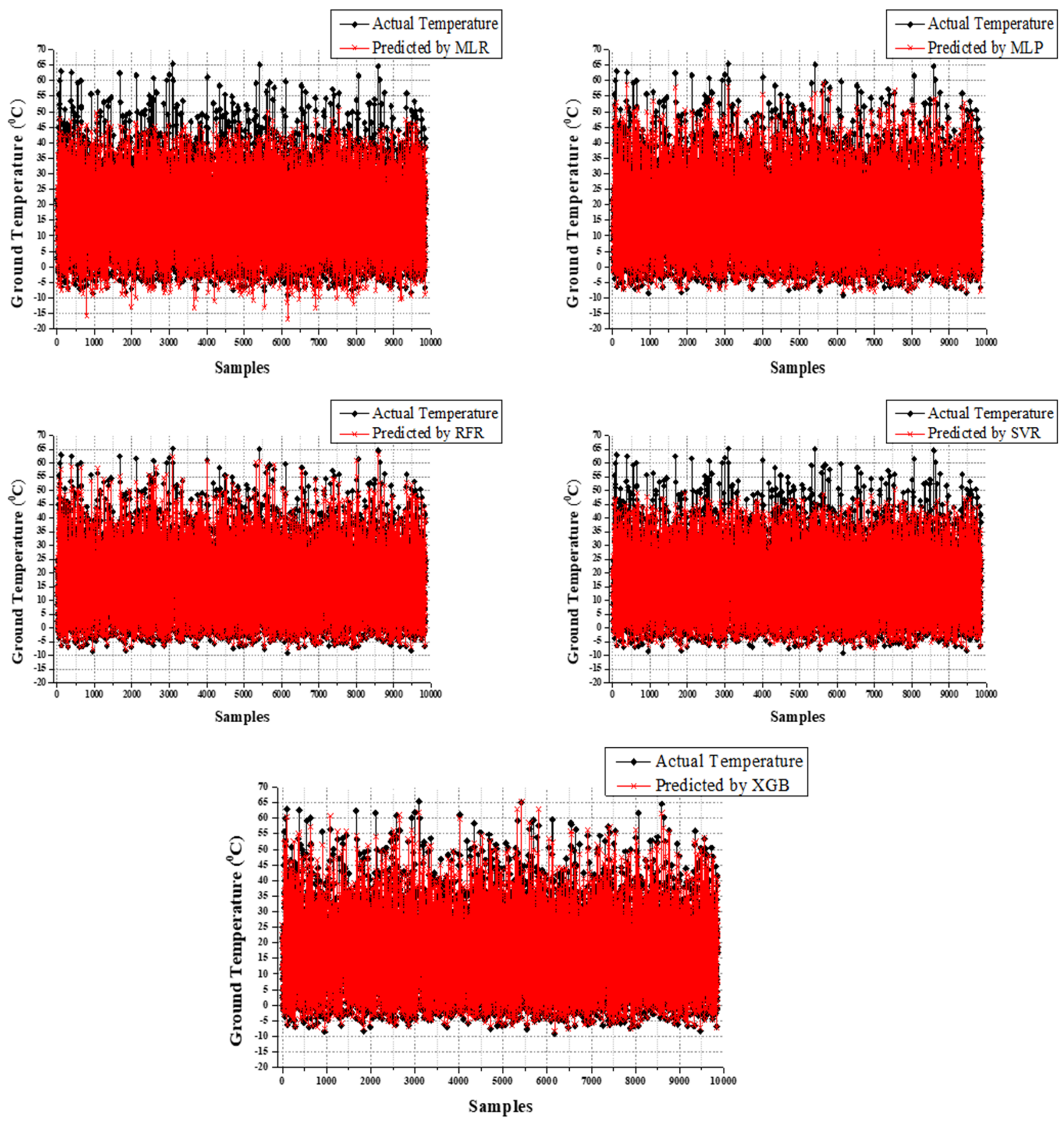
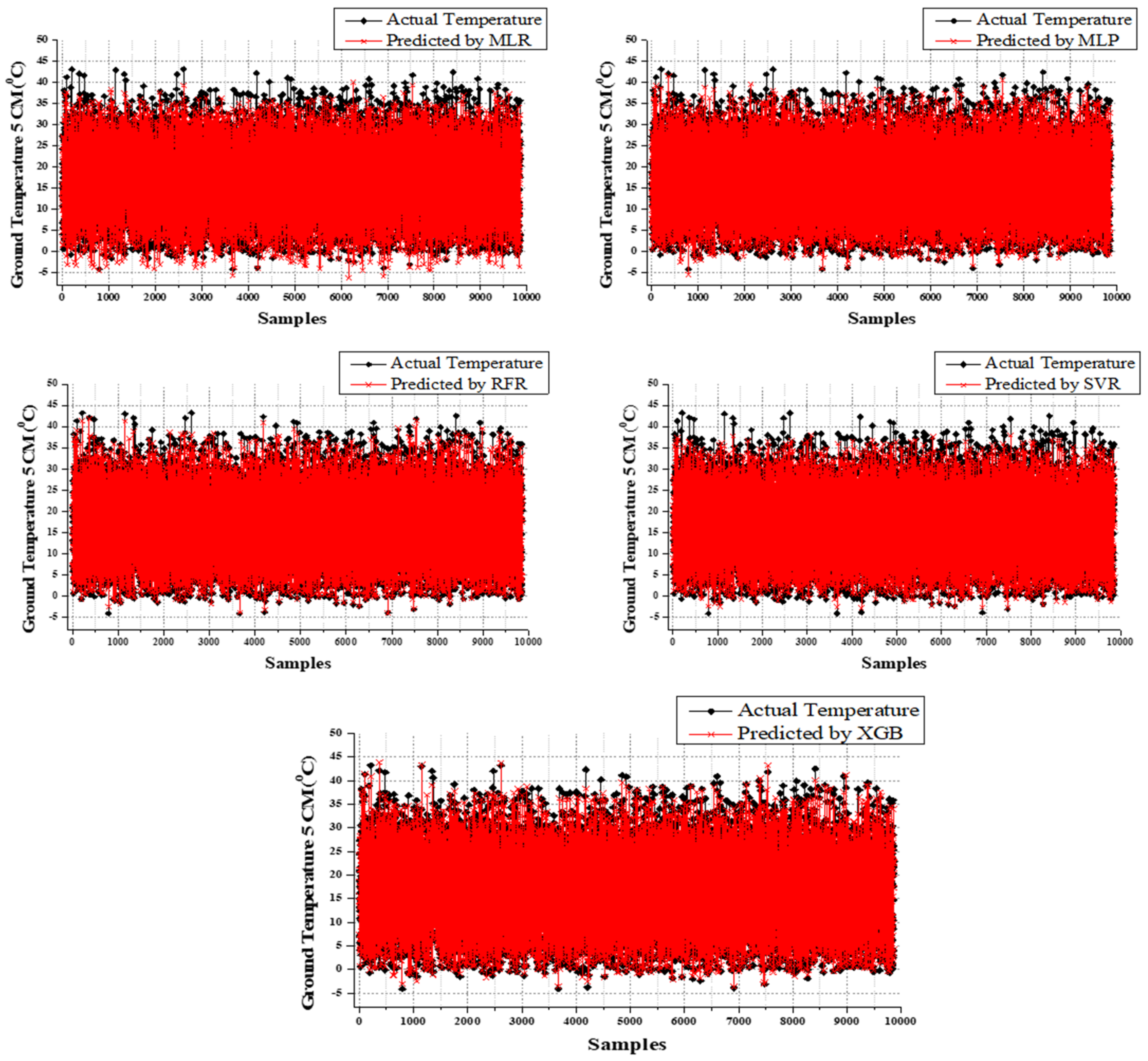
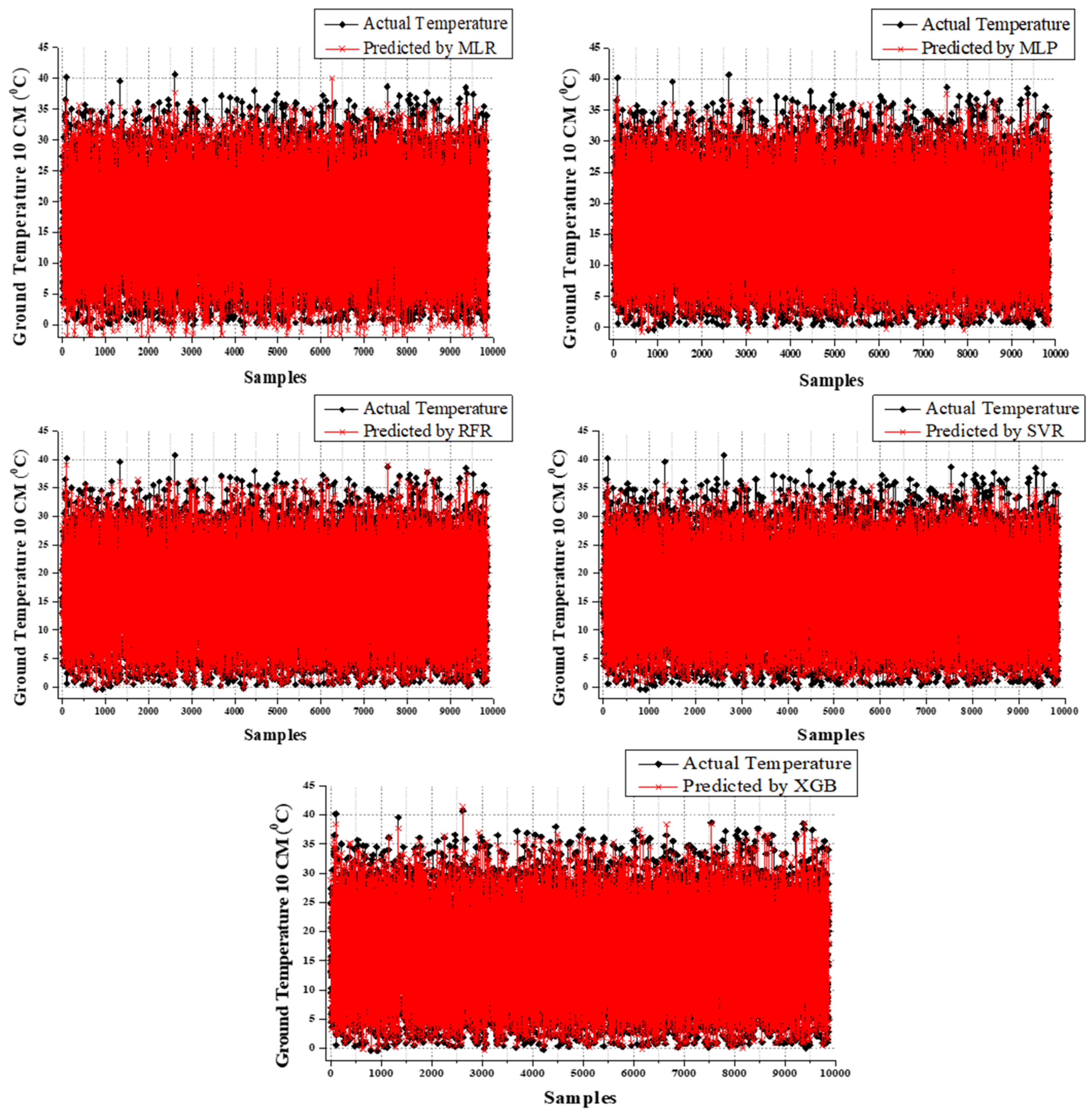
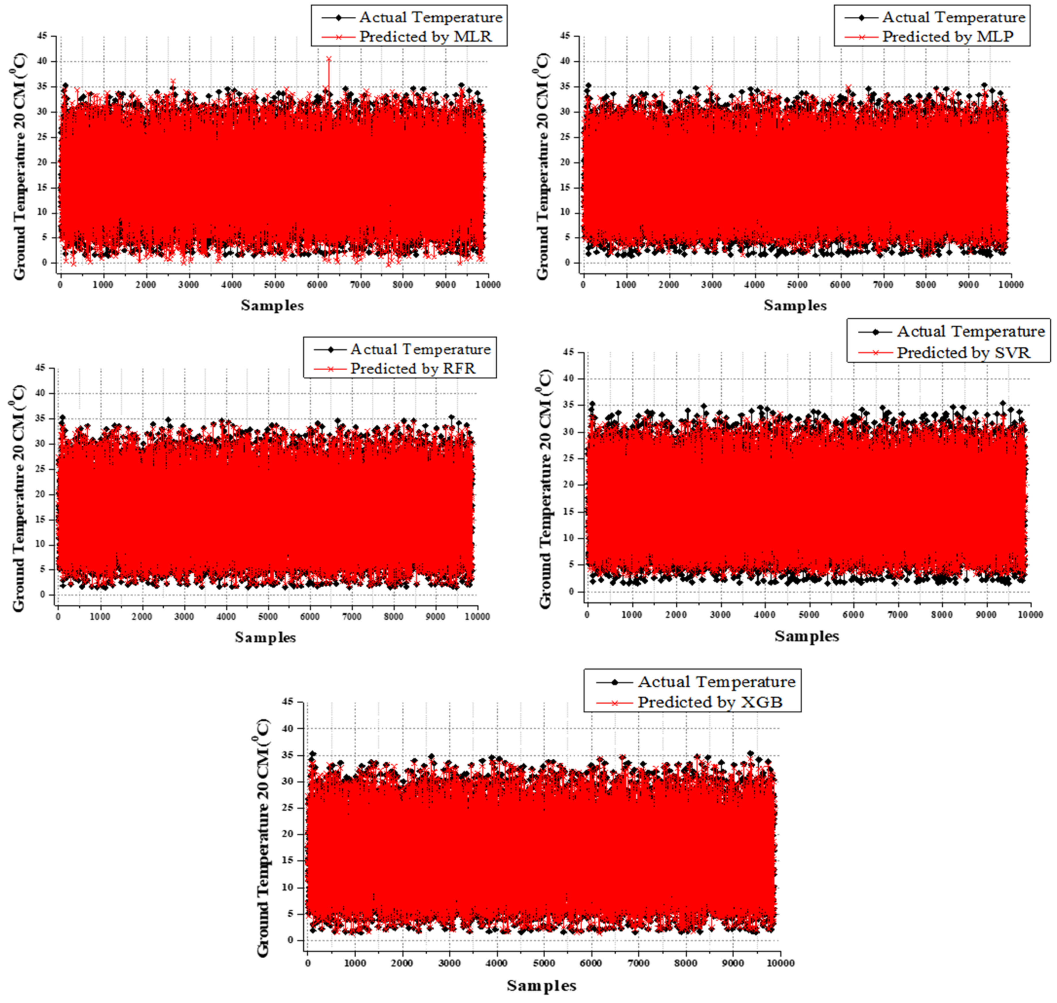
Based on the dataset performance outcomes, the M1 input dataset assists in achieving superior performance from all models for GT predictions except GT_30 predictions. Overall prediction results of both training time and testing time are satisfied in the XGB model. The performance of the five models for GT, GT_5, GT_10, GT_20, and GT_30 is shown in Figure 6, Figure 7, Figure 8, Figure 9 and Figure 10.

For the GT prediction training time, XGB results are comparatively higher (MAE = 0.669, RMSE = 0.915, and R² = 0.993) followed by the MLP (MAE = 1.616, RMSE = 2.42, and R² = 0.957). Other than those models, SVR and MLR performed third and fourth, respectively. Surprisingly, the RFR regression model evidently shows over-fit during the testing time, not only in GT prediction but also in the rest of the predictions (refer to Table 3). Even though RFR performed follow-through of XGB models during the testing time, the reliability is under suspicion due to the over-fit during the training time. Because validation assessment is essential, as mentioned above, the current study considered testing results as the model’s performance. Thus, during the time of testing, XGB outperformed other models (MAE = 1.063, RMSE = 1.679, and R² = 0.978). RFR’s performance followed that of XGB (MAE = 16.086% high, RMSE = 19.475% high, and R² = 0.920% low), and the third, fourth, and fifth performances were from MLP (MAE = 56.914% high, RMSE = 47.409% high, and R² = 2.453% low), SVR (MAE = 70.743% high, RMSE = 75.997% high, and R² = 4.5% low), and MLR (MAE = 201.505% high, RMSE = 146.039% high, and R² = 10.838% low), accordingly. The MLR model suffered to produce a more competitive outcome than the ML-based models for the GT predictions as from the results. The comparison results between the actual values and predicted values are clearly shown in Figure 6.

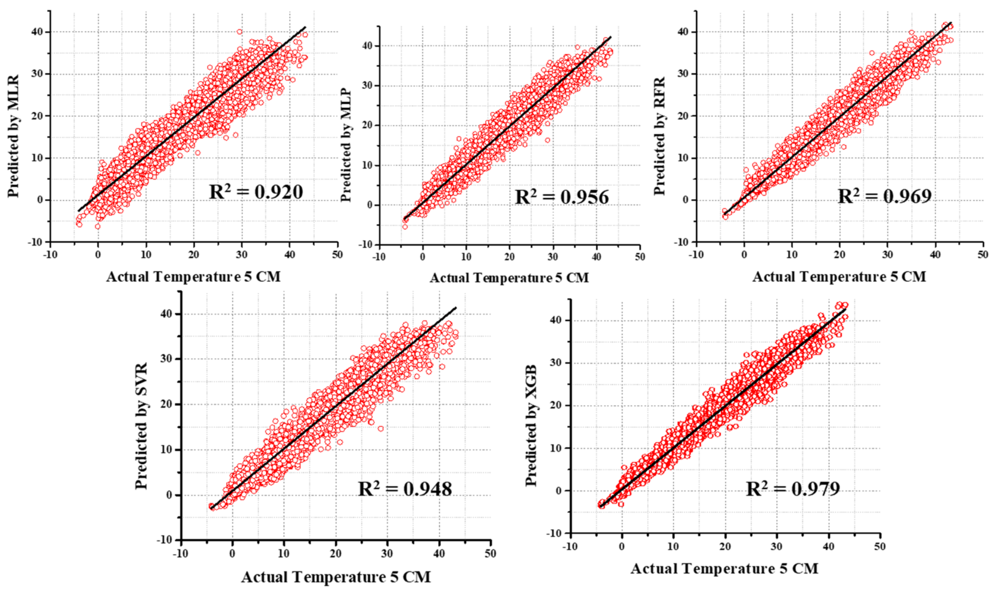
By GT prediction results, the GT_5 followed an akin performance pattern. XGB performance outperformed during the training and testing time of other models. The top performance was achieved from the XGB model for the GT_5 predictions during the training time (MAE = 0.594; RMSE = 0.789; R² = 0.992) and testing time as well (MAE = 0.887; RMSE = 1.263; R² = 0.979). However, according to the training results of GT_5 predictions, MLP, SVR, and MLR retained the second, third, and fourth positions, respectively. According to the testing results, RFR, MLP, SVR, and MLR attained second (21.758% higher MAE, 23.119% higher RMSE, and 1.021% lesser R²), third (56.708% higher MAE, 46.793% higher RMSE, and 2.349% lesser R²), fourth (66.856% higher MAE, 60.807% higher RMSE, and 3.167% lesser R²), and fifth (116.122% higher MAE, 98.337% higher RMSE, and 6.026% lesser R²), respectively (refer to Table 3). As mentioned above, the XGB model attained superior performance during the GT_10 predictions. The results of GT_10 prediction training and testing time were comprehensively explained in Table 3. According to that, the XGB performance overcame the MLP (second), SVR (third), and MLR (fourth) performances, respectively, during the training time. The difference obtained when compared to the XGB model performance were RFR (28.745% higher MAE, 34.731% higher RMSE, and 1.320% lesser R²), MLP (86.234% higher MAE, 75.902% higher RMSE, and 3.248% lesser R²), SVR (92.847% higher MAE, 85.365% higher RMSE, and 3.756% lesser R²), and MLR (146.289% higher MAE, 125.854% higher RMSE, and 6.295% lesser R²).

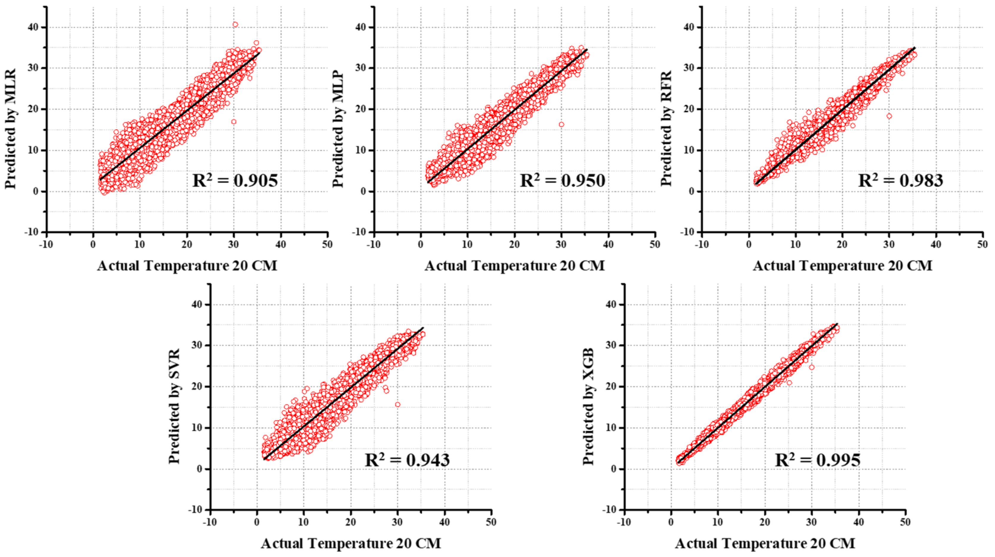
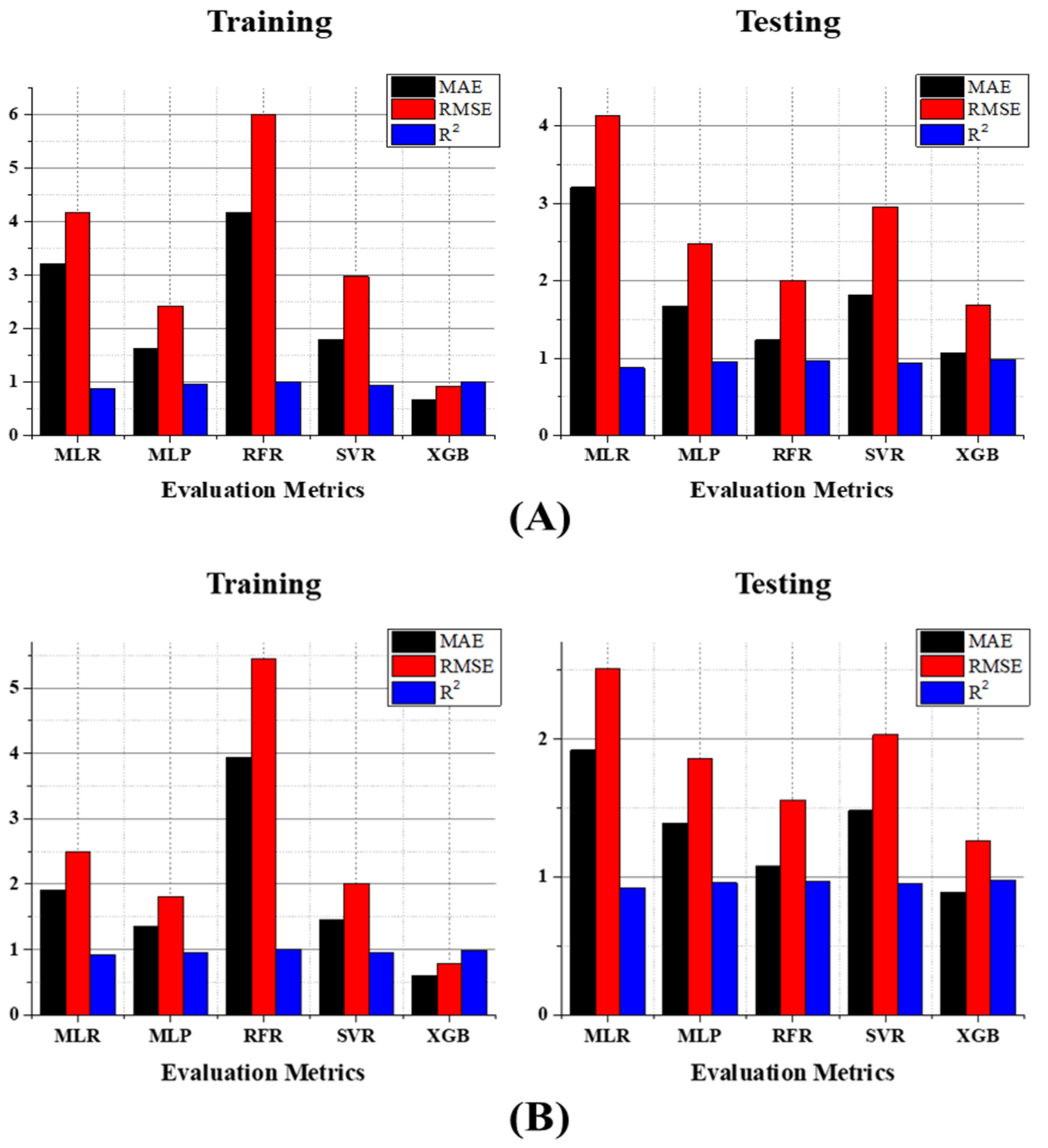
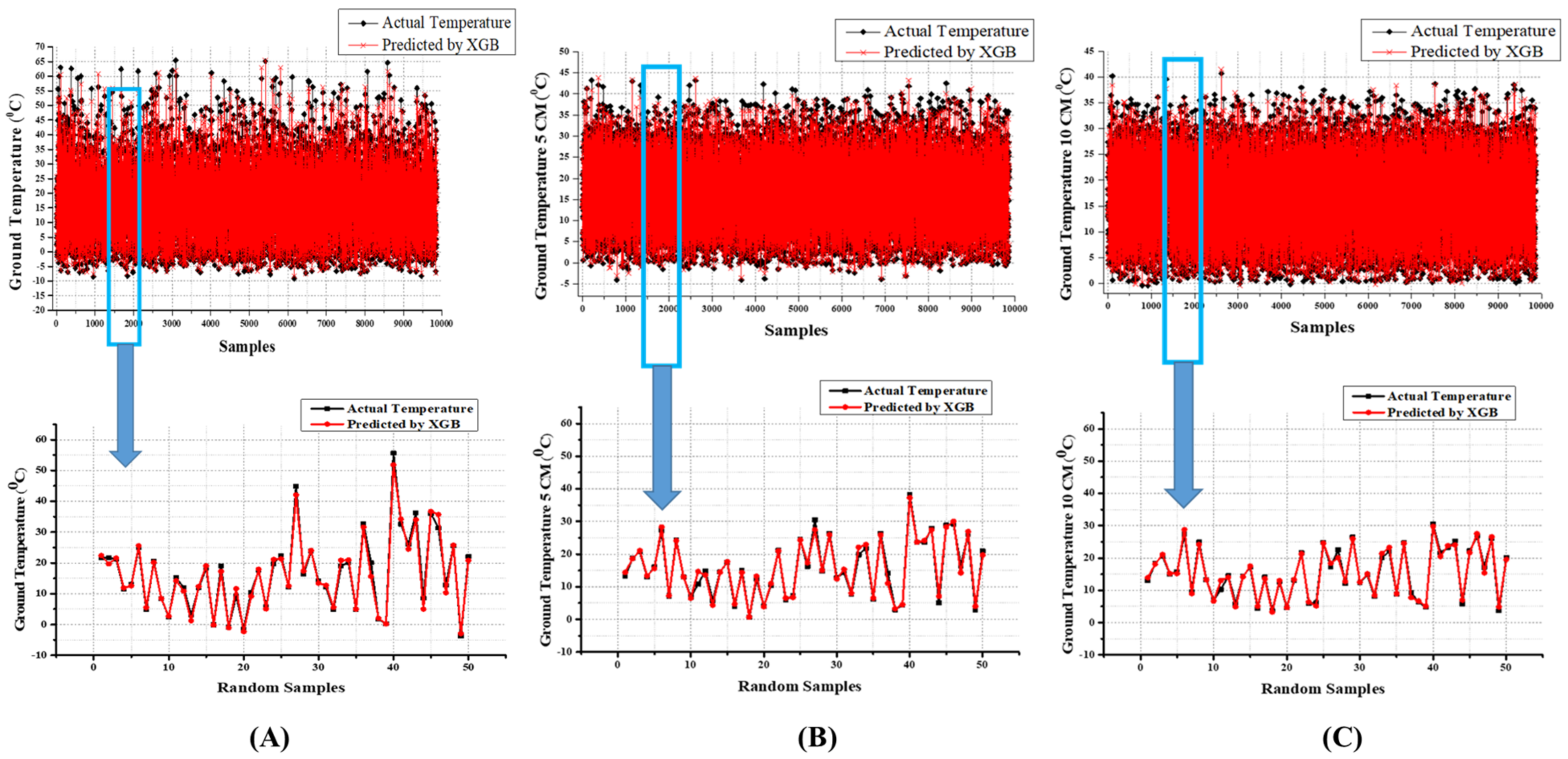
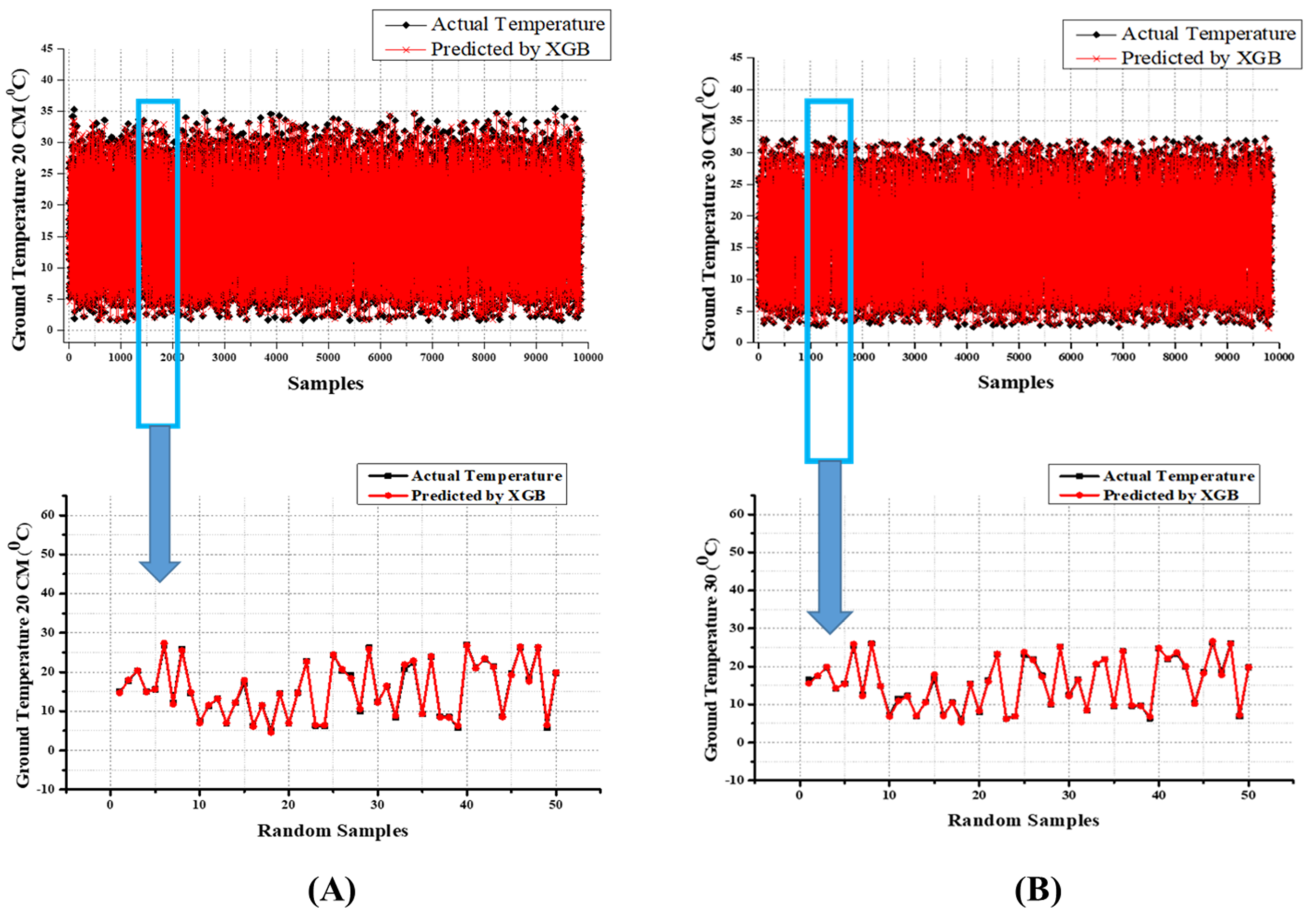
When examining the results of GT_20 predictions, GBR’s results of training time (MAE = 0.286, RMSE = 0.368, and R² = 0.997) and testing time (MAE = 0.416, RMSE = 0.551, and R² = 0.995) were superior, whereas MLP, SVR, and MLR carried out the second, third, and fourth positions. During the testing time, RFR (58.173% higher MAE, 82.94% higher RMSE, and 1.20% lesser R²), MLP (222.837% higher MAE, 214.882% higher RMSE, and 4.523% lesser R²), SVR (237.01% higher MAE, 235.39% higher RMSE, and 5.226% lesser R²), and MLR (356.731% higher MAE, 334.664% higher RMSE, and 9.045% lesser R²) were placed in the second, third, fourth, and fifth positions, respectively. As with other results, the GT_30 prediction results also prove that the models operate in the same way. However, the difference between the superior performing model and the others is developed when the GT depth increases. The GBR executes better results than SVR (75.357% higher MAE, 133.515% higher RMSE, and 1.10% lesser R²), MLP (399.643% higher MAE, 398.09% higher RMSE, and 5.81% lesser R²), SVR (420.357% higher MAE, 427.248% higher RMSE, and 6.5419% lesser R²), and MLR (608.929% higher MAE, 581.471% higher RMSE, and 11.134% lesser R²) during the treating time. During the training time, MLP, SVR, and MLR accomplish second, third, and fourth performance positions, respectively. The scatterplots of predicted and actual values using MLR, MLP, SVR, RFR, and XGB for all GT predictions were shown in Figure 11, Figure 12, Figure 13, Figure 14 and Figure 15. In addition, the comparison of evaluation metric’s results between the training and testing time were displayed in Figure 16 and Figure 17. The comparison of observed and predicted values of 50 random samples to understand clearly using the XGB model for all GT predictions were displayed in Figure 18 and Figure 19.

4. Discussion

Ground or soil temperature (GT) and plant growth are immeasurably associated since the photosynthesis, membrane stability, water and nitrification process, metabolites, and diversity of soil microbial communities are influenced precisely by the GT [11,13,21]. However, the critical aspects for exceptional final quality and quantity of production, such as seed germination, root-growth orientation, root and shoot development, branching, leaf development, and flowering, were predominant dependencies of GT [9,11,13]. Even though GT plays a meaningful role in agricultural production, the direct method of measuring the GT is time-consuming, expensive, and requires human effort. Therefore, the current study uses computational methods to model the GT at different depths. The current study analyzes the performance of prediction models in terms of evaluation metrics with two different datasets. As a result, the M1 dataset helps to model GT more precisely than the M2 except in GT_30 predictions. A previous study [11] conducted a study to model GT at different depths (5, 10, 50, and 100 cm) on a monthly basis with different independent variables as in the present study. That study used advanced ML models such as CART, GMDH, ELM, and ANN models for predicting GT, and the results show that the extreme learning machine (ELM) outperformed the others. Whereas GT at 5, 10, and 50 cm depth predictions was accomplished using one dataset as input, the prediction of GT at 100 cm depth was modeled using different datasets. Such study has a notable variation in evaluation metrics from one dataset (RMSE = 3.211; NSE = 0.749; R² = 0.901) to the other (RMSE = 5.149; NSE = 0.356; R² = 0.459), whereas the present study has no notable fluctuation (MAE is 0.24% lower, RMSE is 1.551% lower, and R² is 0.10% higher in M2 than M1). Modeling multiple dependent variables with a single dataset is a straightforward and evident approach to reducing computational time, cost, and complexity. The present study considers such notations and endorses the M1 as the optimal dataset for predicting GT.

The results show that the mathematical model’s (MLR model) performance is finite during the whole prediction time compared to the computational models (ML model). For instance, the RMSE difference between observed and predicted for the all-computational model was 0.2–2.4 °C, whereas MLR has a difference of 4.1 °C. Even though the mathematical models are straightforward, accessible, and simple to design, they are limited to a scenario of extrapolating beyond the range of data. Such deviations could be solved using computational models since those models are adaptive to the scene due to the essential nature of learning through weights, so the computational models have superiority over standard statistical models. The optimization techniques also induce the prediction values to fit more closely to the observed values. As mentioned in Section 2.4 all other models except MLR have been optimized using hyperparameter tuning (fine-tuning) using the grid-search method. The actual results of native algorithms have been noted, and the same algorithms are subjected to optimal hyperparameter searching then re-trained using the fine-tuned parameters. The current study observed that the model performance was improved after optimization most of the time. The error results also evidenced a marginal improvement in results after the optimization for overall prediction, which concurs with the previous literature. Mostly, the overfitting problems were solved during fine-tuning, but RFR over-fitted during the present examination. Even though the RFR’s nature leads to overfitting, different optimization techniques can solve the issue because more authoritative optimization techniques have been developed recently. Since the objective of the present study is to develop a reliable and straightforward model for GT prediction, the computational time was considered for the main examination; so, the present study used standard optimization techniques. The reason to increase the accuracy when the sensor goes deep into the soil surface is that fluctuations in temperature on top of the soil are frequent. However, according to the Korean metrological society, multiple sensors would have been placed and collected the data. So, the final sensory value of the topsoil surface is elusive, whereas the fluctuations are lesser when the sensor goes into the deep soil.

Extreme GT is catastrophic for soil microorganism development and a plant’s life. Particularly at 32 °C, the plant’s growth will face slowdown, whereas 60 °C leads to the expiration of a plant’s life span [9]. Many types of research [11,33,36] have been conducted to predict the soil temperature in long-term intervals, such as one day, one week, or monthly averages; such cases could be considered as a reference for precautions to avoid extreme GT. If plants suffer from extreme temperatures for a particular period, they may drastically lose moisture absorption capacity, since the soil moisture may decrease by 85% due to evaporation and transpiration [9,32]. The current research tries to amend the shortcomings of previous studies so that we propose a short-term (1 h) prediction model. Few studies have been conducted to predict the different GT depths using ML models in short-term intervals. For instance, a previous study [30] modeled GT in 2 cm, 5 cm, 10 cm, and 20 cm depths with 30 min intervals. That study used relative humidity, air temperature, global solar radiation, wind speed, and vapor pressure deficit (VPD) as inputs for prediction using ELM, GRNN, BPNN, and RFR. The findings show that ELM performs well during all the predictions (2 CM RMSE = 1.74 MAE = 1.37; 5 CM RMSE = 1.85 MAE = 1.44; 10 CM RMSE = 2.05 MAE = 1.60; and 20 CM RMSE = 2.47 MAE = 1.91), which is comparatively less than our proposed model (5 CM RMSE = 1.263 MAE = 0.887; 10 CM RMSE = 1.025 MAE = 0.741; 20 CM RMSE = 0.551 MAE = 0.416). However, the proposed model overcomes that literature not only in terms of error metrics, but also that the referenced literature formed a weather station to model GT, whereas the present literature used government weather data, which are cost-efficient and easy to collect. Even though there are errors in the public dataset, they could be corrected using the preprocessing method. Likewise, a study [33] was conducted to predict GT in 3 different depths (5, 10, and 15 cm) for two different areas where the data were collected from the metrological station as in the present study. That study employed BPNN, LSTM, ELM, GRU, and an optimized GRU model for a 6-h prediction. The literature concluded that their proposed optimized GRU model performed well during the entire prediction. They concluded with the proposed model performing better with the evidence of findings through evolution metrics (RMSE = 1.1012, MAE = 0.7586, R² = 0.9638 for 5 CM; RMSE = 0.7658, MAE = 0.5554, R² = 0.9756 for 10 CM; RMSE = 0.6926, MAE = 0.5435, R² = 0.9799 for 15 CM). Even though the MAE and RMSE are less in the previous studies, the R² results are better in our proposed model (RMSE = 1.263, MAE = 0.887, R² = 0.979 for 5 CM: RMSE = 1.025, MAE = 0.741, R² = 0.985 for 10 CM). In addition, LSTM, ELM, and GRU models come in under the RNN models, which are required, higher graphical processors than the ML models. Generally, those models are popular for voice recognition, natural language processing, and in time series modeling. On the other hand, the previous study [14] utilized EEMD-CNN models, which are more convoluted with deep neural networks to predict the GT in 5, 10, and 30 CM. When compared with the results (RMSE = 1.229, MAE = 1.510, R² = 0.955 for 5 CM; RMSE = 0.879, MAE = 0.686, R² = 0.974 for 10 CM; RMSE = 0.735, MAE = 0.541, R² = 0.978 for 30 CM), as similar to the previously mentioned study, our model performed better in terms of R², which is an essential metric to evaluate data extrapolation. Overall, the present study developed a simple, non-complex, faster, and more versatile model to predict the GT at different depths for a short-term prediction with a minimum number of predictor attributes.

5. Conclusions

Thanks to recent technological breakthroughs, agricultural output may be made more sustainable in the face of food insecurity caused by climate change and global warming. GT is a critical feature for plant development and output; modeling GT may lead to increased productivity and improved irrigation methods. The current study predicts and analyses numerous models and concludes with the important points listed below:

• The XGB model outperforms the other standard ML-based models in any depth GT prediction. Furthermore, the model’s dependability is superior to that of the others.
• In order to develop an optimum model, the input dataset is critical to improving the efficiency of the output. Finding the proper input parameters utilizing feature importance will enhance the model’s maximum efficiency, yet providing a more significant number of input parameters increases model complexity and computational time.
• Tuning the hyperparameters (fine-tuning) of the computational model can significantly enhance efficiency and help overcome overfitting challenges.
• GT modeling has limitations in that GT is not a universal number and can be volatile related to soil color, shape, vegetation cover, physical and chemical characteristics, and location. As a result, developing a worldwide model to anticipate GT is insufficient. The constraints highlighted above can be overcome in future studies.

References

1. Arulmozhi, E.; Moon, B.E.; Basak, J.K.; Sihalath, T.; Park, J.; Kim, H.T. Machine Learning-Based Microclimate Model for Indoor Air Temperature and Relative Humidity Prediction in a Swine Building. Animals 2021, 11, 222. [Google Scholar] [CrossRef] [PubMed]
2. Gornall, J.; Betts, R.; Burke, E.; Clark, R.; Camp, J.; Willett, K.; Wiltshire, A. Implications of Climate Change for Agricultural Productivity in the Early Twenty-First Century. Philos. Trans. R. Soc. B Biol. Sci. 2010, 365, 2973–2989. [Google Scholar] [CrossRef] [PubMed]
3. Arulmozhi, E.; Bhujel, A.; Moon, B.E.; Kim, H.T. The Application of Cameras in Precision Pig Farming: An Overview for Swine-Keeping Professionals. Animals 2021, 11, 2343. [Google Scholar] [CrossRef]
4. Hoegh-Guldberg, O.; Jacob, D.; Taylor, M. Impacts of 1.5°C of Global Warming on Natural and Human Systems. Spec. Rep. Intergov. Panel Clim. Chang. 2018, 175–181. [Google Scholar]
5. Knox, J.; Hess, T.; Daccache, A.; Wheeler, T. Climate Change Impacts on Crop Productivity in Africa and South Asia. Environ. Res. Lett. 2012, 7, 34032. [Google Scholar] [CrossRef]
6. Sultan, B.; Defrance, D.; Iizumi, T. Evidence of Crop Production Losses in West Africa Due to Historical Global Warming in Two Crop Models. Sci. Rep. 2019, 9, 12834. [Google Scholar] [CrossRef] [PubMed] [Green Version]
7. Jia, G.; Shevliakova, E.; Artaxo, P.; De Noblet-Ducoudré, N.; Houghton, R.; Anderegg, W.; Bernier, P.; Carlo Espinoza, J.; Semenov, S.; Xu, X.; et al. Land-Climate Interactions Coordinating. IPCC Rep. 2019, 131–248. [Google Scholar]
8. Gupta, D.; Chowdhury, A.; Rahaman, M.S. Soil Temperature Prediction under Limited Data Condition. Int. J. Curr. Microbiol. Appl. Sci. 2019, 8, 102–112. [Google Scholar] [CrossRef]
9. Sabri, N.S.A.; Zakaria, Z.; Mohamad, S.E.; Jaafar, A.B.; Hara, H. Importance of Soil Temperature for the Growth of Temperate Crops under a Tropical Climate and Functional Role of Soil Microbial Diversity. Microbes Environ. 2018, 33, 144–150. [Google Scholar] [CrossRef] [Green Version]
10. Bilgili, M. The Use of Artificial Neural Networks for Forecasting the Monthly Mean Soil Temperatures in Adana, Turkey. Turkish J. Agric. For. 2011, 35, 83–93. [Google Scholar] [CrossRef]
11. Alizamir, M.; Kisi, O.; Ahmed, A.N.; Mert, C.; Fai, C.M.; Kim, S.; Kim, N.W.; El-Shafie, A. Advanced Machine Learning Model for Better Prediction Accuracy of Soil Temperature at Different Depths. PLoS ONE 2020, 15, e0231055. [Google Scholar] [CrossRef] [PubMed] [Green Version]
12. Hanson, C.L.; Marks, D.; Van Vactor, S.S. Long-Term Climate Database, Reynolds Creek Experimental Watershed, Idaho, United States. Water Resour. Res. 2001, 37, 2839–2841. [Google Scholar] [CrossRef]
13. Jahanfar, A.; Drake, J.; Sleep, B.; Gharabaghi, B. A Modified FAO Evapotranspiration Model for Refined Water Budget Analysis for Green Roof Systems. Ecol. Eng. 2018, 119, 45–53. [Google Scholar] [CrossRef]
14. Hao, H.; Yu, F.; Li, Q. Soil Temperature Prediction Using Convolutional Neural Network Based on Ensemble Empirical Mode Decomposition. IEEE Access 2020, 9, 4084–4096. [Google Scholar] [CrossRef]
15. Tian, Y.; Guan, B.; Zhou, D.; Yu, J.; Li, G.; Lou, Y. Responses of Seed Germination, Seedling Growth, and Seed Yield Traits to Seed Pretreatment in Maize (Zea mays L.). Sci. World J. 2014, 2014, 834630. [Google Scholar] [CrossRef] [Green Version]
16. Onwuka, B. Effects of Soil Temperature on Some Soil Properties and Plant Growth. Adv. Plants Agric. Res. 2018, 8, 34–37. [Google Scholar] [CrossRef]
17. Enrique, G.S.; Braud, I.; Jean-Louis, T.; Michel, V.; Pierre, B.; Jean-Christophe, C. Modelling Heat and Water Exchanges of Fallow Land Covered with Plant-Residue Mulch. Agric. For. Meteorol. 1999, 97, 151–169. [Google Scholar] [CrossRef]
18. Kang, S.; Kim, S.; Oh, S.; Lee, D. Predicting Spatial and Temporal Patterns of Soil Temperature Based on Topography, Surface Cover and Air Temperature. For. Ecol. Manag. 2000, 136, 173–184. [Google Scholar] [CrossRef]
19. Mihalakakou, G. On Estimating Soil Surface Temperature Profiles. Energy Build. 2002, 34, 251–259. [Google Scholar] [CrossRef]
20. Koçak, K.; Şaylan, L.; Eitzinger, J. Nonlinear Prediction of Near-Surface Temperature via Univariate and Multivariate Time Series Embedding. Ecol. Modell. 2004, 173, 1–7. [Google Scholar] [CrossRef]
21. Gaumont-Guay, D.; Black, T.A.; Griffis, T.J.; Barr, A.G.; Jassal, R.S.; Nesic, Z. Interpreting the Dependence of Soil Respiration on Soil Temperature and Water Content in a Boreal Aspen Stand. Agric. For. Meteorol. 2006, 140, 220–235. [Google Scholar] [CrossRef]
22. Gao, Z.; Bian, L.; Hu, Y.; Wang, L.; Fan, J. Determination of Soil Temperature in an Arid Region. J. Arid Environ. 2007, 71, 157–168. [Google Scholar] [CrossRef]
23. Droulia, F.; Lykoudis, S.; Tsiros, I.; Alvertos, N.; Akylas, E.; Garofalakis, I. Ground Temperature Estimations Using Simplified Analytical and Semi-Empirical Approaches. Sol. Energy 2009, 83, 211–219. [Google Scholar] [CrossRef]
24. Prangnell, J.; McGowan, G. Soil Temperature Calculation for Burial Site Analysis. Forensic Sci. Int. 2009, 191, 104–109. [Google Scholar] [CrossRef]
25. Adhikari, R.; Agrawal, R. An Introductory Study on Time Series Modeling and Forecasting Ratnadip Adhikari R. K. Agrawal. arXiv 2013, arXiv:1302.6613. [Google Scholar]
26. Shirvani, A.; Moradi, F.; Moosavi, A.A. Time Series Modelling of Increased Soil Temperature Anomalies during Long Period. Int. Agrophysics 2015, 29, 509–515. [Google Scholar] [CrossRef] [Green Version]
27. Kotu, V.; Deshpande, B. Chapter 12. Time Series Forecasting, 2nd ed.; Morgan Kaufmann: Burlington, MA, USA, 2019; pp. 395–445. [Google Scholar]
28. Patowary, A.N. Monthly Temperature Prediction Based on Arima Model: A Case Study in Dibrugarh Station of Assam, India. Int. J. Adv. Res. Comput. Sci. 2017, 8, 292–298. [Google Scholar] [CrossRef]
29. Samadianfard, S.; Ghorbani, M.A.; Mohammadi, B. Forecasting Soil Temperature at Multiple-Depth with a Hybrid Artificial Neural Network Model Coupled-Hybrid Firefly Optimizer Algorithm. Inf. Process. Agric. 2018, 5, 465–476. [Google Scholar] [CrossRef]
30. Feng, Y.; Cui, N.; Hao, W.; Gao, L.; Gong, D. Estimation of Soil Temperature from Meteorological Data Using Different Machine Learning Models. Geoderma 2019, 338, 67–77. [Google Scholar] [CrossRef]
31. Mehdizadeh, S.; Behmanesh, J.; Khalili, K. Evaluating the Performance of Artificial Intelligence Methods for Estimation of Monthly Mean Soil Temperature without Using Meteorological Data. Environ. Earth Sci. 2017, 76, 325. [Google Scholar] [CrossRef]
32. Mehdizadeh, S.; Ahmadi, F.; Kozekalani Sales, A. Modelling Daily Soil Temperature at Different Depths via the Classical and Hybrid Models. Meteorol. Appl. 2020, 27, e1941. [Google Scholar] [CrossRef]
33. Wang, X.; Li, W.; Li, Q. A New Embedded Estimation Model for Soil Temperature Prediction. Sci. Program. 2021, 2021, 5881018. [Google Scholar] [CrossRef]
34. Feigl, M.; Lebiedzinski, K.; Herrnegger, M.; Schulz, K. Machine-Learning Methods for Stream Water Temperature Prediction. Hydrol. Earth Syst. Sci. 2021, 25, 2951–2977. [Google Scholar] [CrossRef]
35. Sahoo, K.; Samal, A.K.; Pramanik, J.; Pani, S.K. Exploratory Data Analysis Using Python. Int. J. Innov. Technol. Explor. Eng. 2019, 8, 4727–4735. [Google Scholar] [CrossRef]
36. Bilgili, M. Prediction of Soil Temperature Using Regression and Artificial Neural Network Models. Meteorol. Atmos. Phys. 2010, 110, 59–70. [Google Scholar] [CrossRef]
37. Imanian, H.; Cobo, J.H.; Payeur, P.; Shirkhani, H.; Mohammadian, A. A Comprehensive Study of Artificial Intelligence Applications for Soil Temperature Prediction. Preprints 2022, 2022020101. [Google Scholar] [CrossRef]
38. Elanchezhian, A.; Basak, J.K.; Park, J.; Khan, F.; Okyere, F.G.; Lee, Y.; Bhujel, A.; Lee, D.; Sihalath, T.; Kim, H.T. Evaluating Different Models Used for Predicting the Indoor Microclimatic Parameters of a Greenhouse. Appl. Ecol. Environ. Res. 2020, 18, 2141–2161. [Google Scholar] [CrossRef]
39. Taki, M.; Ajabshirchi, Y.; Ranjbar, S.F.; Matloobi, M. Application of Neural Networks and Multiple Regression Models in Greenhouse Climate Estimation. Agric. Eng. Int. CIGR J. 2016, 18, 29–43. [Google Scholar]
40. Ma, X.; Fang, C.; Ji, J. Prediction of Outdoor Air Temperature and Humidity Using Xgboost. IOP Conf. Ser. Earth Environ. Sci. 2020, 427, 12013. [Google Scholar] [CrossRef]
41. Vassallo, D.; Krishnamurthy, R.; Sherman, T.; Fernando, H.J.S. Analysis of Random Forest Modeling Strategies for Multi-Step Wind Speed Forecasting. Energies 2020, 13, 5488. [Google Scholar] [CrossRef]
42. Walker, S.; Khan, W.; Katic, K.; Maassen, W.; Zeiler, W. Accuracy of Different Machine Learning Algorithms and Added-Value of Predicting Aggregated-Level Energy Performance of Commercial Buildings. Energy Build. 2020, 209, 109705. [Google Scholar] [CrossRef]
43. Drucker, H.; Burges, C.J.C.; Kaufman, L.; Smola, A.; Vapnik, V. Support Vector Regression Machines. In Advances in Neural Information Processing Systems; Mozer, M.C., Jordan, M., Petsche, T., Eds.; MIT Press: Cambridge, MA, USA, 1996; p. 9. [Google Scholar]
44. Drucker, H.; Surges, C.J.C.; Kaufman, L.; Smola, A.; Vapnik, V. Support Vector Regression Machines. Adv. Neural Inf. Process. Syst. 1997, 1, 155–161. [Google Scholar]
45. Hasan, N.; Nath, N.C.; Rasel, R.I. A Support Vector Regression Model for Forecasting Rainfall. In Proceedings of the 2015 2nd International Conference on Electrical Information and Communication Technologies (EICT), Khulna, Bangladesh, 10–12 December 2015; pp. 554–559. [Google Scholar] [CrossRef]
46. Wu, J.; Liu, H.; Wei, G.; Song, T.; Zhang, C.; Zhou, H. Flash Flood Forecasting Using Support Vector Regression Model in a Small Mountainous Catchment. Water 2019, 11, 1327. [Google Scholar] [CrossRef] [Green Version]
47. Chen, T.; Guestrin, C. XGBoost: A Scalable Tree Boosting System. In Proceedings of the 22nd ACM SIGKDD International Conference on Knowledge Discovery and Data Mining, San Francisco, CA, USA, 13–17 August 2016; pp. 785–794. [Google Scholar] [CrossRef]
48. Ibrahem Ahmed Osman, A.; Najah Ahmed, A.; Chow, M.F.; Feng Huang, Y.; El-Shafie, A. Extreme Gradient Boosting (Xgboost) Model to Predict the Groundwater Levels in Selangor Malaysia. Ain. Shams Eng. J. 2021, 12, 1545–1556. [Google Scholar] [CrossRef]
49. Dashdondov, K.; Song, M.H. Factorial Analysis for Gas Leakage Risk Predictions from a Vehicle-Based Methane Survey. Appl. Sci. 2022, 12, 115. [Google Scholar] [CrossRef]
50. Vasker Sharma Imputing Missing Data in Hydrology Using Machine Learning Models. Int. J. Eng. Res. 2021, 10, 78–82. [CrossRef]
51. Yoon, H.; Jun, S.C.; Hyun, Y.; Bae, G.O.; Lee, K.K. A Comparative Study of Artificial Neural Networks and Support Vector Machines for Predicting Groundwater Levels in a Coastal Aquifer. J. Hydrol. 2011, 396, 128–138. [Google Scholar] [CrossRef]
52. Che, Z.; Purushotham, S.; Cho, K.; Sontag, D.; Liu, Y. Recurrent Neural Networks for Multivariate Time Series with Missing Values. Sci. Rep. 2018, 8, 6085. [Google Scholar] [CrossRef] [Green Version]
53. Sattari, M.T.; Avram, A.; Apaydin, H.; Matei, O. Soil Temperature Estimation with Meteorological Parameters by Using Tree-Based Hybrid Data Mining Models. Mathematics 2020, 8, 1407. [Google Scholar] [CrossRef]
Figure 1. The location and geographical information of the metrological station in Busan (Highlighted in map), South Korea (35°06′19.0″ N, 129°01′55.8″ E).
Atmosphere 14 00068 g001
Figure 2. Variations in GT at 5 cm, 10 cm, 20 cm, and 30 cm.
Atmosphere 14 00068 g002
Figure 3. Graphical representation of GT, GT_5, GT_10, GT_20, and GT_30 prediction using machine-learning algorithms.
Atmosphere 14 00068 g003
Figure 4. (A) Pearson heat correlation map of GT; (B) Pearson heat correlation map of GT_5.
Atmosphere 14 00068 g004
Figure 5. (A) Pearson heat correlation map of GT_10; (B) Pearson heat correlation map of GT_20; (C) Pearson heat correlation map of GT_30.
Atmosphere 14 00068 g005
Figure 6. Comparison of observed and predicted values using MLR, MLP, SVR, and XGB for GT.
Atmosphere 14 00068 g006
Figure 7. Comparison of observed and predicted values using MLR, MLP, SVR, and XGB for GT_5.
Atmosphere 14 00068 g007
Figure 8. Comparison of observed and predicted values using MLR, MLP, SVR, and XGB for GT_10.
Atmosphere 14 00068 g008
Figure 9. Comparison of observed and predicted values using MLR, MLP, SVR, and XGB for GT_20.
Atmosphere 14 00068 g009
Figure 10. Comparison of observed and predicted values using MLR, MLP, SVR, and XGB for GT_30.
Atmosphere 14 00068 g010
Figure 11. The scatterplots of predicted and actual values using MLR, MLP, SVR, RFR, and XGB for GT predictions.
Atmosphere 14 00068 g011
Figure 12. The scatterplots of predicted and actual values using MLR, MLP, SVR, RFR, and XGB for GT_5 predictions.
Atmosphere 14 00068 g012
Figure 13. The scatterplots of predicted and actual values using MLR, MLP, SVR, RFR, and XGB for GT_10 predictions.
Atmosphere 14 00068 g013
Figure 14. The scatterplots of predicted and actual values using MLR, MLP, SVR, RFR, and XGB for GT_20 predictions.
Atmosphere 14 00068 g014
Figure 15. The scatterplots of predicted and actual values using MLR, MLP, SVR, RFR, and XGB for GT_30 predictions.
Atmosphere 14 00068 g015
Figure 16. (A) The evaluation metrics results of MLR, MLP, SVR, RFR, and XGB for GT prediction; (B) the evaluation metrics results of MLR, MLP, SVR, RFR, and XGB for GT_5 predictions.
Atmosphere 14 00068 g016
Figure 17. (A) The evaluation metrics results of MLR, MLP, SVR, RFR, and XGB for GT_10 predictions; (B) the evaluation metrics results of MLR, MLP, SVR, RFR, and XGB for GT_20 predictions; (C) the evaluation metrics results of MLR, MLP, SVR, RFR, and XGB for GT_30 prediction.
Atmosphere 14 00068 g017
Figure 18. (A) The comparison of observed and predicted values of 50 random samples to understand clearly using the XGB model for GT predictions; (B) the comparison of observed and predicted values of 50 random samples to understand clearly using the XGB model for GT_5 predictions; (C) the comparison of observed and predicted values of 50 random samples to understand clearly using the XGB model for GT_10 predictions.
Atmosphere 14 00068 g018
Figure 19. (A) The comparison of observed and predicted values of 50 random samples to understand clearly using the XGB model for GT_20 predictions; (B) the comparison of observed and predicted values of 50 random samples to understand clearly using the XGB model for GT_30 prediction.
Atmosphere 14 00068 g019