Abstract
In the storm surge model, the wind drag coefficient Cd is a critical parameter that has a great influence on the forecast of the storm surge level. In the present study, the effect of various wind drag coefficient parameterizations on the storm surge level is investigated in the Bohai Sea, Yellow Sea and East China Sea for Typhoons 7203 and 7303. Firstly, the impacts of initial values of a and b in the linear expression Cd = (a + b × U10) × 10−3 on the pure storm surge model are evaluated based on the data assimilation method. Results indicate that when a and b (i.e., the wind drag coefficients given by Smith, Wu, Geernaert et al. and Mel et al.) are non-zeros, the performance of the model has little difference, and the result from Wu is slightly better. However, they are superior to the performance of the model adopting zero initial values. Then, we discuss the influences of diverse ways of calculating wind drag coefficients, which are inverted by data assimilation method (including both linear and constant Cd) and given in the form of linear formulas, on simulating pure storm surge level. They show that the data assimilation-based coefficients greatly exceed those of the ordinary coefficient formulas. Moreover, the wind drag coefficient in the linear form is a little better than that in constant form when the data assimilation method is used. Finally, the assessment of the impact of astronomical tides on the storm surge level is conducted, and the simulation demonstrates that the storm surge model, which has the combination of four constituents (M2, S2, K1, O1) and wind drag coefficient inverted by the data assimilation method with the linear Cd, exhibits the best performance.
1. Introduction
Storm surge induced by typhoon is one of the most destructive natural hazards in the coastal areas. Surges can be further exacerbated when they come across astronomical tides [1,2,3,4,5,6,7,8]. The combination of storm surge and astronomical tide can bring about a severe flood disaster that may destroy the coastal infrastructure and threaten life safety in the catchment areas [9,10,11,12,13]. In the last decade, the economic loss caused by storm surge disasters averagely accounted for over 90% of the total direct economic losses resulting from all kinds of marine disasters, such as storm surge, sea wave, sea ice, red tide, green tide and so on (Bulletin of China Marine Disaster, http://www.mnr.gov.cn/sj/sjfw/hy/gbgg/zghyzhgb/ (accessed on 24 December 2022)). Consequently, it is imperative to enhance the forecasting capability of the storm surge model in order to reduce the impact of flooding hazards.
In recent years, many researchers have explored storm surge predictions using artificial intelligence methods [14,15,16,17,18]. Lee used the neural network method to predict storm surge level, and the results showed that the neural network can efficiently forecast storm surges [14]. Support vector regression (SVR) was applied to predict the storm surges by Rajasekaran et al., and the comparison between the numerical methods and neural network indicated that storm surges can be efficiently predicted using the SVR [15]. Granata and Nunno used the machine learning algorithm: Regression Tree, Random Forest and Multilayer Perceptron, to forecast the tide levels in Venice. These artificial intelligence models proved able to forecast the tide levels in Venice with good accuracy [17].
Wind stress is one of the major driving forces in the upper ocean, and the wind drag coefficient is a critical parameter in the wind stress equation. Since their beginnings, studies of wind drag coefficient have been ongoing [19,20,21,22,23,24,25,26,27,28,29,30,31]. Earlier researchers have revealed the variations of wind drag coefficient in virtue of observed data from laboratory work and field measurements, and proposed that the wind drag coefficient is linearly related to wind speed (U10) at 10 m height above sea surface, that is, Cd = (a + b × U10) × 10−3 [19,21,22]. It is worth noting that parameters a and b determined by different researchers are very diverse, demonstrating that the linear parameterization of the wind drag coefficient has a large uncertainty. Afterwards, the wind drag coefficient formulated by piecewise function [23,27] or quadratic curve [24,25,28] were developed based on different methods and observations. Using the recorded observations during a major tropical cyclone, Jarosz et al. discussed the momentum transfer at the air–sea interface in terms of the wind drag coefficient, which was represented by quadratic curve and achieved its peak at about 32 m/s for the wind speed [24]. Zijlema et al. used a large number of observations to develop a new parameterization for the wind drag coefficient in the form of a second order polynomial as a function of wind speed [25]. In order to investigate the drag coefficient for higher wind speeds, Cao et al. applied observations from the South China Sea during typhoons to the SWAN wave model and obtained a piecewise function for the drag coefficient [27]. By adding a wind-drag multiplier to the wind drag coefficient formula in a lake hydrodynamic model, Chen et al. developed a modified model with a wind-drag multiplier; their simulations showed that the calibrated model resolved the underestimation problem of lake current speed [29]. As the wind setup is not disturbed by a tidal wave in a closed lagoon, Mel et al. achieved a robust calibration of wind drag coefficient for moderate wind speed. Further, they gave the best-fitting wind drag coefficient that increases linearly with the wind speed in shallow water [30]. Shankar and Behera used the enhanced Wave Boundary Layer Model to estimate the wind drag coefficient and constructed a wind drag coefficient of cubic function for any simulated wind speed [31]; the results showed that the improved wind drag coefficient method performed better than the other two methods [25,32] in estimating the significant storm wave heights and peak surge levels.
With the development of ocean observation and remote sensing technology, more and more marine data have become available. As an important tool to combine the observed data and numerical model, the data assimilation method has been widely used in oceanographic and atmospheric forecasting in the past several decades [33,34,35,36,37,38,39,40,41]. Combining a tangent linear model with an adjoint model of Princeton Ocean Model, Peng and Xie built a four-dimensional variational data assimilation algorithm. They found that improvements in storm surge forecasting are very obvious when assimilating water level alone or together with surface currents [35]. Peng et al. adopted the adjoint data assimilation methodology to discuss the influence of initial condition (IC) and surface boundary condition on coastal storm surge modelling, and the results showed that it was better to adjust both conditions at the same time during adjoint data assimilation [36]. Analogously, in order to increase the storm surge forecasting performance, Li et al. simultaneously optimized the IC and wind drag coefficient (Cd) according to the data assimilation method. Results showed that the model, when adjusting IC and Cd together, performed better than models in which only one of these were adjusted [39]. Using an adjoint-free data assimilation method, Zheng et al. investigated the wind drag coefficient in the German Bight and found that the wind drag coefficient was linearly related to the wind speed in deep water, but largely varied because of the wave shoaling effect in shallow water [40]. Xu et al. used the data assimilation method to explore the wind drag coefficients in the Bohai Sea, Yellow Sea and East China Sea based on the linear expression, indicating that the performance of data assimilation method-based coefficients were superior to those from normal drag coefficient formulas [41].
This study aims to evaluate the impacts of different initial values of a and b in the linear expression Cd, as well as other wind drag coefficient parameterizations, on the pure storm surge elevations in the Bohai Sea, Yellow Sea and East China Sea for Typhoons 7203 and 7303. For the first purpose, five experiments were designed for the zero and non-zero coefficients given by Smith [19], Wu [21], Geernaert et al. [22] and Mel et al. [30] based on the data assimilation method. Then, we constructed four experiments to investigate the effect of wind drag coefficient parameterizations, which were inverted by the data assimilation method with both linear and constant Cd and given by linear Cd formulas, on the storm surge simulation. Finally, in the process of data assimilation, we also explored the performance of the storm surge model when considering the astronomical tide, taking four constituents (M2, S2, K1, O1) as an example.
The numerical model and adjoint model of storm surge, including the astronomical tide, the drag coefficient expressions, experimental designs and model verification, are presented in the second section. The third section consists of three issues: the impact of the initial values of a and b on the storm surge model, the influence of ways of calculating wind drag coefficient and astronomical tide on the storm surge level. The conclusion and discussion are given in the last section.
2. Materials and Methods
2.1. Typhoons and Stations
Typhoon 7203 (Rita) originated in the waters of Micronesia on 5 July 1972, developed into a tropical depression on July 6 and a severe tropical storm on July 7. About two days later, Rita reached super typhoon force. Then, it began to move northwest and enter the East China Sea with typhoon status at about 08:00 on 25 July. After gradually weakening into a severe tropical storm, it landed in Shidao Town of Rongcheng City around 15:00 p.m. on 26 July, with an instantaneous wind speed of 30 m/s and a central pressure of 970 hPa. Subsequently, it passed through the Shandong Peninsula, entered into the Bohai Bay and made landfall in Tianjin. Finally, Typhoon 7203 crossed over the Yanshan Mountain and disappeared in the Inner Mongolian Plateau on July 30. Counting from the beginning of the tropical disturbance, Rita had a life of 26 days, making it the longest typhoon in history. Of course, it brought severe storm surge hazards along the coastal areas, resulting in huge economic losses and casualties.
Typhoon 7303 (Billie) originated in the Philippine Sea on 11 July 1973. After four days, Billie moved northward, alternately classified as a strong typhoon and super typhoon. It reduced to typhoon at about 02:00 on 18 July, and continued tracking northward via the East China Sea, the Yellow Sea and the Bohai Sea. Ultimately, Typhoon 7303 vanished in Inner Mongolia on 20 July. In 2011, the Typhoon Meari followed a similar path to Typhoon 7303.
In this study, the selected time periods and routes of Typhoons 7203 and 7303 can be seen in Figure 1, and data regarding their tracks, central pressures and maximum wind speeds (Table 1 and Table 2) are from the Wenzhou Typhoon Network (http://www.wztf121.com/ (accessed on 24 December 2022)). The intersecting routes of Typhoons 7203 and 7303 may produce some important results. And these results could provide a significant basis for the environmental assessment of a nuclear power plant site in Liaodong Bay. The positions of 10 tidal stations are also shown in Figure 1.
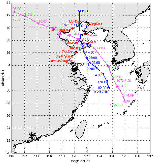
Figure 1.
Typhoon routes and positions of tidal stations. Mauve and blue solid lines denote the routes of Typhoons 7203 and 7303, respectively. Circles represent the Local Standard Time. Red asterisks show the positions of 10 tidal stations.

Table 1.
Best track, central pressure, and maximum wind speed for Typhoon 7203.
Table 2.
Best track, central pressure, and maximum wind speed for Typhoon 7303.
2.2. Coupled Tide-Surge Numerical Model and Adjoint Assimilation Model
The coupled tide-surge numerical model is based on a two-dimensional depth-averaged flow model, consisting of a continuity equation and momentum equations. In the right-handed Cartesian coordinate system, the governing equations used in this model are as follows.
where t is time, h is resting water depth, ζ is surface elevation, u and v are velocity components in the east (x) and north (y), respectively, f is Coriolis parameter, k is bottom friction coefficient, A is horizontal eddy viscosity coefficient, g is gravitational acceleration, is the adjusted height of equilibrium tides, ρw is sea water density, ρa is air density, Cd is surface wind drag coefficient, Pa is sea surface pressure, (Wx, Wy) is surface wind field.
The pressure field and wind field used in the governing Equations (2) and (3) are adopted according to Jelesnianski [42]. The former (i.e., the pressure field) expression is
where r is distance between the storm center and grid center, R is maximum typhoon wind speed radius, Pa is pressure at r of sea surface, P0 is typhoon center pressure, P∞ is ambient pressure.
The latter (i.e., the wind field) is
where i and j are, respectively, eastward and northward unit vectors, Vox and Voy are moving velocities of the storm center, and WR is maximum wind speed.
where (x, y) and (xc, yc) are, respectively, coordinates of grid center and storm center, and θ is inflow angle,
When the above-mentioned model is together driven by both tidal forcing and atmospheric forcing, it is called a coupled tide-surge model. If the model is only driven by atmospheric forcing, it is named a pure storm surge model, while if the model is only driven by tidal forcing, it is called a tide model.
Usually, the storm surge model composed of the governing equations and boundary conditions is solvable and the solution is unique. Nevertheless, the storm surge levels calculated by numerical model are not as good as the observed data, like altimeter data and tidal stations data. The errors between them can be caused by the governing equations, boundary conditions, approximate hypotheses, truncation error of computer and so on. In the present study, we adopt the data assimilation method to reduce the errors between the simulated and observed levels, and the Lagrange multipliers method is preferred.
To formulate the adjoint equations, we define the Lagrangian function as follows
where Kζ is constant, ζ is simulation, is observation, ζa, ua and va are the adjoint variables of ζ, u and v, respectively.
Similar to the method of He et al. [33], we can gain the following adjoint equations
2.3. Wind Drag Coefficient
In the upper ocean, the wind stress near the sea surface plays an important role in driving ocean circulation, generating sea surface waves and causing storm surge. Additionally, the wind drag coefficient Cd is a critical parameterization for calculating the wind stress. Generally, the wind drag coefficient Cd depends on the wind speed, water depth, topography, wve age, and so on [26,43]. In previous studies, the wind drag coefficient was usually expressed as a linear increase of wind speed at 10 m above the sea surface [19,21,22,30]. Afterwards, for different wind speed ranges, the wind drag coefficient was formulated in the form of a piecewise function [23,27]. In addition, many researchers developed a second-order polynomical for the wind drag coefficient [25,28]. As the wind speed strengthens, the wind drag coefficient Cd firstly increases, after reaching the peak, and then decreases, appearing in a shape of parabola.
In the present paper, the selected four drag coefficient formulas [19,21,22,30] are as follows. If the wind speeds are outside the given ranges in Formulas (12)–(15), the wind drag coefficient is set as a constant (0.0026).
There exists a linear relationship between the wind drag coefficient Cd and wind speed U10 given by the formula of Smith [19], Wu [21], Geernaert et al. [22] and Mel et al. [30]. Among them, the first three Formulas (12)–(14) are widely used. The last one (15) is obtained by optimizing the coefficients in a linear expression of Cd in seven storm events for the Venice Lagoon. These four formulas will be substituted into the numerical model of storm surge to calculate the pure storm surge level.
In addition, we will also investigate the data assimilation method with Lagrangian multiplier for both the constant Cd and the linear expression Cd = (a + b × U10) × 10−3, where empirical parameters a and b are commonly determined by observed data [23,36]. In the first case, Cd is directly inverted when giving a constant initial value, and in the other case, the coefficients a and b from the formula Cd = (a + b × U10) × 10−3 are inverted with given initial values. Finally, we assess the impact of initial values of a and b on the pure storm surge model, and examine the spatial distribution of the wind drag coefficient in some sea areas.
2.4. Experimental Designs, Model Setting and Model Verification
2.4.1. Experimental Designs
In this paper, we designed three sets of experiments to calculate the storm surge level. Firstly, based on the data assimilation method, we evaluated the impact of the initial values of a and b for experiments E1–E5 (Table 3) on the pure storm surge model. In E1, we take zeros as the initial values of a and b; in E2–E4, the initial a and b values are from conventional Formulas (12)–(15). Secondly, the influence of ways of calculating wind drag coefficient on pure storm surge level was investigated in E5, E6, E7 and E8 (Table 3). In E6, Cd is directly inverted by the data assimilation method, at an initial value of 0.0026; in E7 and E8, the wind drag coefficient formula was substituted into the storm surge numerical model to calculate the storm surge level. Finally, we discussed the effect of four constituents (M2, S2, K1, O1) on the storm surge level in the process of data assimilation, namely, experiment E9 (Table 3).
Table 3.
Experiments evaluating the effect of initial values of a and b in the expression Cd, data assimilation method and four constituents (M2, S2, K1, O1) on the storm surge level.
2.4.2. Model Setting
The storm surge model involving the astronomical tide used in this paper covered an area of the Bohai Sea, Yellow Sea and East China Sea, ranging from 117.5° E to 130.5° E and from 24.5° N to 41° N, with a grid resolution of 5′ × 5′. The Taiwan Strait and the first island chains were selected as the open boundary conditions, where the astronomical tide was provided by four constituents (M2, S2, K1, O1) in E9. Simultaneously, it is assumed that no water had flowed into or away from the seacoast along the closed boundaries. In all seas, the bottom drag coefficient was taken as a constant (0.0016) and the sea surface level and current velocity were 0 at the initial time. Arakawa C grid, that is, the water level is in the center of grid and current velocity is at the edge, is applied to the model. The time step is set to 60 s. Additionally, the typhoon process was divided into several stages, and each stage is 6 h, that is, the assimilation window is set to 6 h. The observations from 10 tide stations are used in the model during Typhoons 7203 and 7303, and all the observations are used both for assimilation and for validation.
2.4.3. Model Verification
When the atmospheric forcing term, that is, the surface wind field (Wx, Wy) and pressure field Pa, is removed from the governing Equations (2) and (3), the numerical model involving the astronomical tide is degraded into the tide model of Lu et al. [44]. In the tide model, the tidal potential and open boundary conditions are the driving force. Here, the tidal potential is calculated by Fang et al. [45], and the water level on the open boundary is computed by He et al. [33].
The tide model was run on 27 April 1972 and the duration was 90 days. The simulated results of the last 60 days were used for the harmonic analysis. The absolute mean error of amplitude and phase-lag in the sea surface elevation are, respectively, (3.2 cm, 4.6°) and (3.3 cm, 4.0°) between the simulation and observation at the 489 points of TOPEX/Poseidon (T/P) tracks (Figure 2) using remote sensing technology for the M2 and S2 constituents. For example, the absolute mean errors of amplitude and phase-lag in Longkou station are, respectively, (0.0897 cm, 0.8138°) and (0.0629 cm, 3.9687°) for the M2 and S2 constituents, and they are, respectively, (0.2831 cm, 1.758°) and (0.1142 cm, 0.4949°) for the M2 and S2 constituents in Qingdao station. These results are acceptable for the present study. The cotidal charts of M2 and S2 constituents can be seen in Figure 3.
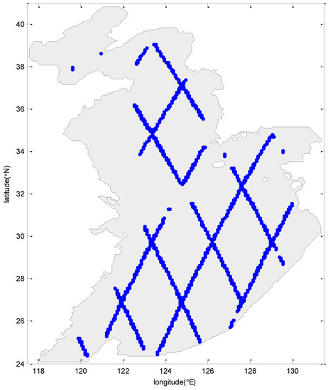
Figure 2.
Blue dots mean the locations of TOPEX/Poseidon observation points.
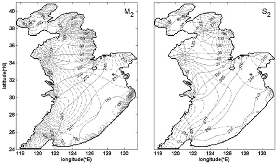
Figure 3.
Computed cotidal charts for the M2 and S2 constituents. Solid line denotes the phase-lag (in deg), and dotted line denotes the amplitude (in m) in [0.1 3.0] m, taken 0.1 m as the interval length.
3. Results and Discussion
3.1. Impact of the Initial Values of a and b on Pure Storm Surge Model
In the process of data assimilation, we investigate the impact of initial values of a and b in formula Cd on the pure storm surge model. Table 3 provides the initial values of a and b in experiments E1–E5. The root–mean–square (RMS) errors between simulated and observed storm surge levels are listed in Table 4 for Typhoons 7203 and 7303. The RMS errors at 10 tidal stations are shown in Table 5. The results indicate that the performances of the pure storm surge model have little difference in experiments E2–E5 and they are better than that in E1. Taking Typhoon 7203 as an example, the mean RMS errors for 10 tidal stations in E2–E5 are 12.0 cm, 12.1 cm, 12.0 cm and 12.0 cm, which is 26.38%, 25.77%, 26.38% and 26.38% less than that in E1, respectively. This is probably because the initial values of a and b in E2–E5 have no significant difference. At the same time, taking the LongKou tidal station for Typhoon 7203 and ShiJiuSuo tidal station for Typhoon 7303 as an example, the relative errors between the simulated and observed storm surge levels in each period in E1–E5 are listed in Table 6. The time series of simulated levels and observations and the differences between them are shown in Figure 4 and Figure 5 at LongKou station for Typhoon 7203 and at ShiJiuSuo station for Typhoon 7303, respectively. These results also lead to similar conclusions. Hence, the influence of the zero and non-zero initial values of a and b on the pure storm surge model is distinct when the data assimilation method is used. In the subsequent section, we will choose the coefficients in E5 as the initial value of a and b because of their smaller RMS error and relative error.
Table 4.
Root–mean–square errors between simulated and observed storm surge levels in each 6-h period during Typhoons 7203 and 7303 (unit: cm).
Table 5.
Root–mean–square errors between simulated and observed storm surge levels at 10 tidal stations during Typhoons 7203 and 7303 (unit: cm).
Table 6.
Relative errors between simulated and observed storm surge levels at LongKou and ShiJiuSuo tidal stations in each 6-hour period during Typhoons 7203 and 7303 (unit: %).
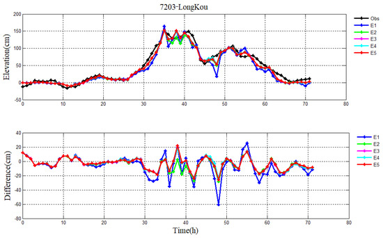
Figure 4.
Pure storm surge levels in experiments E1−E5, observation (black line) (top), and their differences (bottom) during Typhoon 7203 at LongKou station.
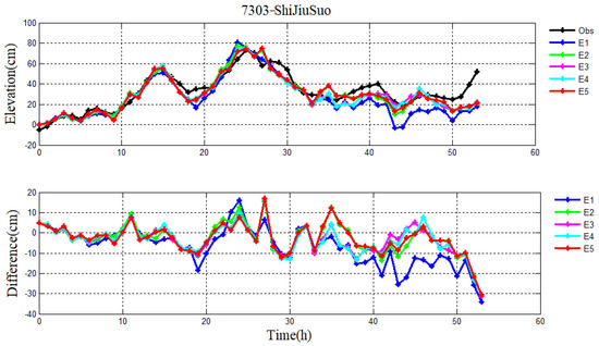
Figure 5.
Pure storm surge levels in experiments E1−E5, observation (black line) (top), and their differences (bottom) during Typhoon 7303 at ShiJiuSuo station.
3.2. Spatial Distribution of Wind Drag Coefficients during Typhoons 7203 and 7303
In the present section, we compare the wind drag coefficients calculated by the formula and the data assimilation method. The spatial distributions of wind drag coefficients at 20:00 p.m. on 26 July 1972 (for Typhoon 7203) and at 14:00 p.m. on 19 July 1973 (for Typhoon 7303) calculated from the experiments E5–E8 are shown in Figure 6 and Figure 7, respectively. The magnitudes and extreme value distributions can be clearly seen in Figure 6 and Figure 7. The extremums of wind drag coefficients inverted by the data assimilation method in E5 and E6 (Figure 6a,b and Figure 7a,b) mainly arise in the Bohai Sea and the North Yellow Sea, especially on the coast. However, in the open sea (i.e., the East China Sea), the wind drag coefficient in E5 changes slowly, and it is almost a constant in E6. The difference is that when the data assimilation method is used, the wind drag coefficient in E5 is related to the wind speed, while it is an independent value in E6. Therefore, compared to the wind drag coefficient in E6, the spatial distribution of Cd in E5 gradually varies, which is attributed to the use of the circular wind field from Jelesnianski [42]. Relatively, there are less differences between E7 and E8: the minimum of wind drag coefficient in E7 and E8 (Figure 6c,d and Figure 7c,d) is in the center of typhoon, and the maximum is around the typhoon eye, gradually decreasing from the middle to the edge. The characteristic of the spatially distributed wind drag coefficient in E7 and E8 is largely associated with the selected circular wind field given by Jelesnianski [42]. Furthermore, the Cd calculated by data assimilation method in E5 and E6 is totally different from those in E7–E8 in shallow water, such as the Bohai Sea and Yellow Sea. In addition, we also found that the larger wind drag coefficient is located in the right of the storm migration direction (Figure 6), which is ascribed to the asymmetric wind distribution. This result is consistent with that given by Moon et al. [46].

Figure 6.
Spatial distributions of the calculated drag coefficients in E5−E8 (a–d) at 20:00 p.m. on 26 July 1972 during Typhoon 7203.
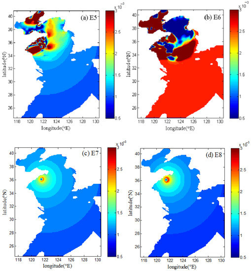
Figure 7.
Spatial distributions of the calculated drag coefficients in E5−E8 (a–d) at 14:00 p.m. on 19 July 1973 during Typhoon 7303.
Differences in spatial distribution of wind drag coefficient will affect the evaluation of wind stress, as well as the pure storm surge level. In the following study, we will investigate the comparison between the simulations of pure storm surge model in experiments E5–E8 and observations during Typhoons 7203 and 7303.
3.3. Influence of the Way of Calculating Wind Drag Coefficient on the Pure Storm Surge Level
We explore the influence of different ways of calculating wind drag coefficient on the pure storm surge level without the astronomical tides in this section. In experiment E5, the pure storm surge levels are simulated by using the data assimilation method, and the initial values of a and b in the parameterization formula Cd are taken from Wu [21] during Typhoons 7203 and 7303. Different from the experiment E5, the initial value of Cd in E6 is constant (0.0026) in the process of data assimilation. Whereas, two wind drag coefficient formulas in Equations (13) and (15) (i.e., E7–E8, without optimization) are used in the numerical model of pure storm surge to calculate the water level. The RMS errors between the simulations and observations of storm surge levels in each period during Typhoons 7203 and 7303 are illustrated in Table 7. The mean values of RMS errors are 11.2 cm, 13.6 cm, 27.4 cm and 28.1 cm for Typhoon 7203 and 16.0 cm, 19.0 cm, 29.1 cm and 29.3 cm for Typhoon 7303 in E5–E8, respectively. The result in E5 has the best performance, followed by that in E6. This suggests that the wind drag coefficient in a linear form is better than that in a constant form when the data assimilation method is used, but they are both superior to the results in E7–E8, which adopted the linear wind drag coefficient form but did not employ the data assimilation method. Analogously, the results at 10 tidal stations (Table 8) also demonstrate that the data assimilation method has obvious advantages compared to the parameterization formula without data assimilation.
Table 7.
Root–mean–square errors between simulated and observed storm surge levels in each 6-hour period during Typhoons 7203 and 7303 (unit: cm).
Table 8.
Root–mean–square errors between simulated and observed storm surge levels at 10 tidal stations during Typhoons 7203 and 7303 (unit: cm).
Spatially distributed water levels calculated by the pure storm surge model in E5–E8 can be seen in Figure 8 and Figure 9. Results show that there are some differences in the storm surge levels between the parameterization formula and data assimilation method, particularly in Figure 8 and Figure 9b. Furthermore, the water levels vary significantly in the Bohai Sea and coastal regions but change slowly in exposed waters. Figure 10, Figure 11, Figure 12 and Figure 13 demonstrate the time sequences of simulated pure storm surge levels without the astronomical tides and observations and differences between them at the YanTai and LianYunGang tidal stations for Typhoons 7203 and 7303, respectively. Compared to the water levels calculated by wind drag coefficient formula (i.e., E7–E8), the water levels simulated by data assimilation method in E5–E6 are closer to the observations. And the result in E5 is slightly better than that in E6.
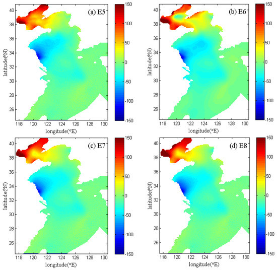
Figure 8.
Spatially distributed levels calculated by the pure storm surge model in E5–E8 at 02:00 p.m. on 27 July 1972 during Typhoon 7203.
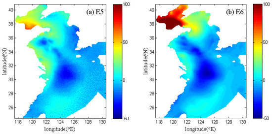
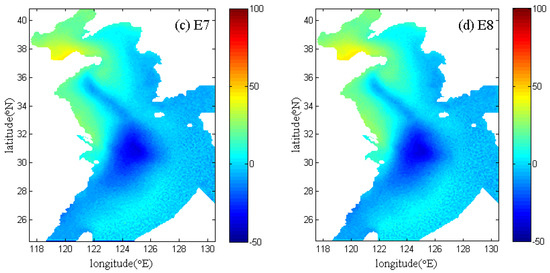
Figure 9.
Spatially distributed levels calculated by the pure storm surge model in E5–E8 at 20:00 a.m. on 19 July 1973 during Typhoon 7303.
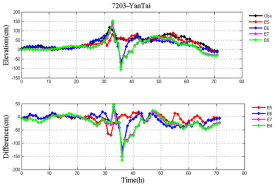
Figure 10.
Pure storm surge levels without the astronomical tides in E5−E8, observation (black line) (top), and their differences (bottom) during Typhoon 7203 at YanTai station.
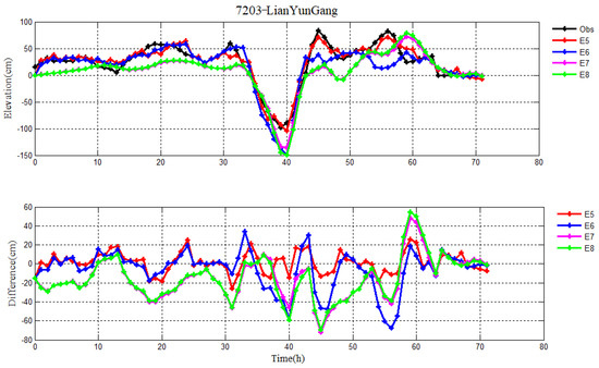
Figure 11.
Pure storm surge levels without the astronomical tides in E5−E8, observation (black line) (top), and their differences (bottom) during Typhoon 7203 at LianYunGang station.
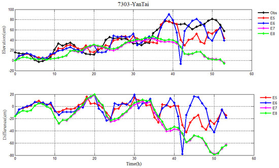
Figure 12.
Pure storm surge levels without the astronomical tides in E5−E8, observation (black line) (top), and their differences (bottom) during Typhoon 7303 at YanTai station.
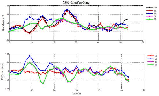
Figure 13.
Pure storm surge levels without the astronomical tides in E5−E8, observation (black line) (top), and their differences (bottom) during Typhoon 7303 at LianYunGang station.
In addition, taking the YanTai tidal station for instance, the variation of observed levels has an obvious distinction when Typhoons 7203 and 7303 arrive at YanTai station (Figure 10 and Figure 12). Although the wind direction of Typhoon 7203 at YanTai station is to the northwest, the reduction of observed level reaches up to 50 cm. However, the decrease of value is 11 cm for Typhoon 7303, where the wind direction is to the north at YanTai station. The primary reason for this distinction is that the maximum wind speed is different, namely, 30 m/s for Typhoon 7203 and 15 m/s for Typhoon 7303, respectively.
3.4. Influence of the Astronomical Tide on the Storm Surge Level
In this section, the influence of the astronomical tide on storm surge level is discussed for Typhoons 7203 and 7303. Here, we take four constituents (M2, S2, K1, O1) as an example and conduct another experiment, namely, E9. When the data assimilation method is used, the initial values of a and b from the linear formula Cd in E5 and E9 are the same as Wu [21]. Table 9 lists the RMS errors between the simulations and observations of storm surge levels in each period in E5 and E9. The mean values of RMS errors are 11.2 cm and 10.0 cm for Typhoon 7203 and 16.0 cm and 14.6 cm for Typhoon 7303, respectively. The RMS errors at 10 tidal stations can be seen in Table 10. These results suggest that the simulated storm surge levels from E9 are closer to the observations when the four constituents (M2, S2, K1, O1) are considered. Figure 14 and Figure 15 show the time series of simulated and observed water levels and their differences at the RuShan tidal station for Typhoons 7203 and 7303, respectively. Meanwhile, taking the RuShan tidal station for Typhoons 7203 and 7303 as an example, the relative errors between the simulated and observed storm surge levels in each period in E5 and E9 are listed in Table 11. They confirm that the astronomical tide should be considered in the storm surge model.
Table 9.
Root–mean–square errors between simulated and observed storm surge levels in each 6-hour period during Typhoons 7203 and 7303 (unit: cm).
Table 10.
Root–mean–square errors between simulated and observed storm surge levels at 10 tidal stations during Typhoons 7203 and 7303 (unit: cm).
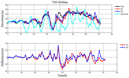
Figure 14.
Storm surge levels without and with four constituents (M2, S2, K1, O1) in E5 and E9, respectively; observation (black line), total level of combination with the astronomical tide and storm surge (cyan line) (top), and their differences (bottom) during Typhoon 7203 at RuShan station.
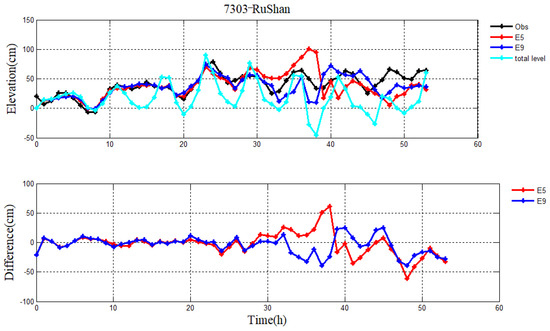
Figure 15.
Storm surge levels without and with four constituents (M2, S2, K1, O1) in E5 and E9 respectively, observation (black line), total level of combination with the astronomical tide and storm surge (cyan line) (top), and their differences (bottom) during Typhoon 7303 at RuShan station.
Table 11.
Relative errors between simulated and observed storm surge levels at RuShan tidal station in each 6-hour period during Typhoons 7203 and 7303 (unit: %).
4. Conclusions
The storm surge caused by a typhoon generally threatens coastal areas, and the forecast ability of a storm surge model largely depends on the parameterization of wind drag coefficient. In this paper, we investigated the impact of initial values of a and b in formula of Cd on the pure storm surge model in the process of data assimilation. Additionally, we evaluated the effect of different methods for calculating wind drag coefficient on the pure storm surge model. Finally, the performance of the storm surge model involving the astronomical tide was discussed based on the data assimilation method.
To assess the impact of the initial values of a and b on the pure storm surge model, the coefficients from Smith, Wu, Geernaert et al. and Mel et al. (i.e., non-zeros in E2–E5) and zeros (E1) were employed. Using the data assimilation method, the RMS errors between the simulated and observed water levels during Typhoons 7203 and 7303 had little difference when a and b were non-zeros, and the performance of the model in E5 is slightly better. Nevertheless, these results were better than that in E1. Therefore, the zero and non-zero initial values of a and b can result in different pure storm surge levels. We should choose the appropriate initial values for a and b in Cd when the data assimilation method is used.
Further, during Typhoons 7203 and 7303, we designed four experiments to evaluate the wind drag coefficient parameterizations: (1) the drag coefficient inverted by using the data assimilation method with a linear function for Cd (E5); (2) the drag coefficient inverted by using the data assimilation method with constant Cd (E6); (3) the linear drag coefficient formulas from Wu [21] (E7) and Mel [30] (E8). The results showed that the effectiveness of the data assimilation method was far better than that of the wind drag coefficient formulas. Therefore, the advantage of the data assimilation method is quite evident for simulating the storm surge level. Besides, the wind drag coefficient employing the linear form is slightly better than a constant wind drag coefficient in the process of data assimilation.
Finally, we added the four constituents (M2, S2, K1, O1) to the storm surge model by using the data assimilation method during Typhoons 7203 and 7303. We found that the simulations of storm surge levels were closer to the observed data when considering the M2, S2, K1 and O1 constituents. Hence, the role of the astronomical tide should be taken into account in predicting storm surge levels.
Author Contributions
Conceptualization, J.X.; methodology, W.S. and Y.N.; software, K.M. and J.X.; formal analysis, Y.N. and X.B.; writing—original draft preparation, J.X.; writing—review and editing, C.L.; supervision, X.L.; funding acquisition, C.L., W.S. and X.L. All authors have read and agreed to the published version of the manuscript.
Funding
This research was funded by the National Natural Science Foundation of China, grant numbers 41606006, 41806219, and U1806214, the National key research and development program, grant numbers 2018YFC1407602 and 2019YFC1408405, and the Strategic Priority Research Program of Chinese Academy of Sciences (XDB42000000).
Institutional Review Board Statement
Not applicable.
Informed Consent Statement
Not applicable.
Data Availability Statement
Typhoons 7203 and 7303 data used in this paper was collected from Wenzhou Typhoon Network, this data can be found here: http://www.wztf121.com/ (accessed on 3 April 2022).
Conflicts of Interest
The authors declare no conflict of interest.
References
- Fleming, J.G.; Fulcher, C.W.; Luettich, R.A.; Estrade, B.D.; Allen, G.D.; Winer, H.S. A real time storm surge forecasting system using ADCIRC. In Estuarine and Coastal Modeling; ASCE: Reston, VA, USA, 2007; pp. 893–912. [Google Scholar]
- Dietrich, J.C.; Zijlema, M.; Westerink, J.J.; Holthuijsen, L.H.; Dawson, C.; Luettich, R.A., Jr.; Jensen, R.E.; Smith, J.M.; Stelling, G.S.; Stone, G.W. Modeling hurricane waves and storm surge using integrally-coupled, scalable computations. Coast. Eng. 2011, 58, 45–65. [Google Scholar] [CrossRef]
- Maspataud, A.; Ruz, M.H.; Vanhée, S. Potential impacts of extreme storm surges on a low-lying densely populated coastline: The case of Dunkirk area, Northern France. Nat. Hazards 2013, 66, 1327–1343. [Google Scholar] [CrossRef]
- Olbert, A.I.; Nash, S.; Cunnane, C.; Hartnett, M. Tide-surge interactions and their effects on total sea levels on total sea level in Irish coastal waters. Ocean Dyn. 2013, 63, 599–614. [Google Scholar] [CrossRef]
- Xu, J.L.; Zhang, Y.H.; Cao, A.Z.; Liu, Q.; Lv, X.Q. Effects of tide-surge interactions on storm surges along the coast of the Bohai Sea, Yellow Sea, and East China Sea. Sci. China Earth Sci. 2016, 59, 1308–1316. [Google Scholar] [CrossRef]
- Chu, D.D.; Zhang, J.C.; Wu, Y.S.; Jiao, X.H.; Qian, S.H. Sensitivities of modelling storm surge to bottom friction, wind drag coefficient, and meteorological product in the East China Sea. Estuar. Coast Shelf Sci. 2019, 231, 106460. [Google Scholar] [CrossRef]
- Du, M.; Hou, Y.J.; Hu, P.; Wang, K. Effects of typhoon paths on storm surge and coastal inundation in the Pearl River Estuary, China. Remote Sens. 2020, 12, 1851. [Google Scholar] [CrossRef]
- Guo, Y.X.; Hou, Y.J.; Liu, z.; Du, M. Risk prediction of coastal hazards induced by typhoon: A case study in the coastal region of Shenzhen, China. Remote Sens. 2020, 12, 1731. [Google Scholar] [CrossRef]
- Lin, N.; Emanuel, K.; Oppenheimer, M.; Vanmarcke, E. Physically based assessment of hurricane surge threat under climate change. Nat. Clim. Change 2012, 2, 462–467. [Google Scholar] [CrossRef]
- Haigh, I.D.; Wijeratne, E.M.S.; MacPherson, L.R.; Pattiaratchi, C.B.; Mason, M.S.; Crompton, R.P.; George, S. Estimating present day extreme water level exceedance probabilities around the coastline of Australia: Tides, extra-tropical storm surges and mean sea level. Clim. Dyn. 2014, 42, 121–138. [Google Scholar] [CrossRef]
- Chen, W.B.; Chen, H.; Hisao, S.C.; Chang, C.H.; Lin, L.Y. Wind forcing effect on hindcasting of typhoon-driven extreme waves. Ocean Eng. 2019, 188, 106260. [Google Scholar] [CrossRef]
- He, Z.G.; Tang, Y.L.; Xia, Y.Z.; Chen, B.D.; Xu, J.; Yu, Z.Z.; Li, L. Interaction impacts of tides, waves and winds on storm surge in a channel-island system: Observational and numerical study in Yangshan Harbor. Ocean Dynam. 2020, 70, 307–325. [Google Scholar] [CrossRef]
- Hisao, S.C.; Chen, H.; Wu, H.L.; Chen, W.B.; Chang, C.H.; Guo, W.D.; Chen, Y.M.; Lin, L.Y. Numerical simulation of large wave heights from super Typhoon Neparktak (2016) in the Eastern waters of Taiwan. J. Mar. Sci. Eng. 2020, 8, 217. [Google Scholar] [CrossRef]
- Lee, T.L. Neural network prediction of a storm surge. Ocean Eng. 2006, 33, 483–494. [Google Scholar] [CrossRef]
- Rajasekaran, S.; Gayathri, S.; Lee, T.L. Support vector regression methodology for storm surge predictions. Ocean Eng. 2008, 35, 1578–1587. [Google Scholar] [CrossRef]
- Nunno, F.D.; Granata, F.; Gargano, R.; Marinis, G. Forecasting of extreme storm tide events using NARX neural network-based models. Atmosphere 2021, 12, 512. [Google Scholar] [CrossRef]
- Granata, F.; Nunno, F.D. Artificial Intelligence models for prediction of the tide level in Venice. Stoch. Environ. Res. Risk Assess. 2021, 35, 2537–2548. [Google Scholar] [CrossRef]
- Lee, J.W.; Irish, J.L.; Bensi, M.T.; Marcy, D.C. Rapid prediction of peak storm surge from tropical cyclone track time series using machine learning. Coast. Eng. 2021, 170, 104024. [Google Scholar] [CrossRef]
- Smith, S.D. Wind stress and heat flux over the ocean in Gale force winds. J. Phys. Oceangr. 1980, 10, 709–726. [Google Scholar] [CrossRef]
- Large, W.G.; Pond, S. Open ocean momentum flux measurements in moderate to strong winds. J. Phys. Oceangr. 1981, 11, 324–336. [Google Scholar] [CrossRef]
- Wu, J. Wind-stress coefficients over sea surface from breeze to hurricane. J. Geophys. Res.-Oceans 1982, 87, 9704–9706. [Google Scholar] [CrossRef]
- Geernaert, G.L.; Large, S.E.; Hansen, F. Measurements of the wind stress, heat flux, and turbulence intensity during storm conditions over the North Sea. J. Geophys. Res. Ocean. 1987, 92, 13127–13139. [Google Scholar] [CrossRef]
- Yelland, M.; Taylor, P.K. Wind stress measurements from the open ocean. J. Phys. Oceangr. 1996, 26, 541–558. [Google Scholar] [CrossRef]
- Jarosz, E.; Mitchell, D.A.; Wang, D.W.; Teague, W.J. Bottom-up determination of air-sea momentum exchange under a major tropical cyclone. Science 2007, 315, 1707–1709. [Google Scholar] [CrossRef] [PubMed]
- Zijlema, M.; Van Vledder, G.P.; Holthuijsen, L.H. Bottom friction and wind drag for wave models. Coast Eng. 2012, 65, 19–26. [Google Scholar] [CrossRef]
- Zhao, Z.K.; Liu, C.X.; Li, Q.; Dai, G.F.; Song, Q.T.; Lv, W.H. Typhoon air-sea drag coefficient in coastal regions. J. Geophys. Res. Ocean. 2015, 120, 716–727. [Google Scholar] [CrossRef]
- Cao, H.Q.; Zhou, L.M.; Li, S.Q.; Wang, Z.F. Observation and numerical experiments for drag coefficient under typhoon wind forcing. J. Ocean Univ. China 2017, 16, 35–41. [Google Scholar] [CrossRef]
- Zou, Z.S.; Zhao, D.L.; Tian, J.W.; Liu, B.; Huang, J. Drag coefficient derived from ocean current and temperature profiles at high wind speeds. Tellus A 2018, 70, 1463805. [Google Scholar] [CrossRef]
- Chen, F.; Zhang, C.; Brett, M.T.; Nielsen, J.M. The importance of the wind-drag coefficient parameterization for hydrodynamic modeling of a large shallow lake. Ecol. Inform. 2020, 59, 101106. [Google Scholar] [CrossRef]
- Mel, R.A.; Viero, D.P.; Carniello, L.; Defina, A.; D’Alpaos, L. The first operations of Mo.S.E. System to prevent the flooding of Venice: Insights on the hydrodynamics of a regulated lagoon. Estuar. Coast Shelf Sci. 2021, 261, 107547. [Google Scholar] [CrossRef]
- Shankar, C.G.; Behera, M.R. Improved wind drag formulation for numerical storm wave and surge modeling. Dynam. Atmos. Ocean. 2021, 93, 101193. [Google Scholar] [CrossRef]
- Garratt, J.R. Review of drag coefficients over oceans and continents. Mon. Weather Rev. 1977, 105, 915–929. [Google Scholar] [CrossRef]
- He, Y.J.; Lu, X.Q.; Qiu, Z.F.; Zhao, J.P. Shallow water tidal constituents in the Bohai Sea and the Yellow Sea from a numerical adjoint model with TOPEX/POSEIDON altimeter data. Cont. Shelf Res. 2004, 24, 1521–1529. [Google Scholar] [CrossRef]
- Lionello, P.; Sanna, A.; Elvini, E.; Mufato, R. A data assimilation procedure for operational prediction of storm surge in the northern Adriatic Sea. Cont. Shelf Res. 2006, 26, 539–553. [Google Scholar] [CrossRef]
- Peng, S.Q.; Xie, L.A. Effect of determining initial conditions by four-dimensional variational data assimilation on storm surge forecasting. Ocean Model. 2006, 14, 1–18. [Google Scholar] [CrossRef]
- Peng, S.Q.; Xie, L.A.; Pietrafesa, L.J. Correcting the errors in the initial conditions and wind stress in storm surge simulation using an adjoint optimal technique. Ocean Model. 2007, 18, 175–193. [Google Scholar] [CrossRef]
- Fan, L.L.; Liu, M.M.; Chen, H.B.; Lv, X.Q. Numerical study on the spatially varying drag coefficient in simulation of storm surges employing the adjoint method. J. Oceanol. Limnol. 2011, 29, 702–717. [Google Scholar] [CrossRef]
- Zhang, J.C.; Lu, X.Q.; Wang, P.; Wang, Y.P. Study on linear and nonlinear bottom friction parameterizations for regional tidal models using data assimilation. Cont. Shelf Res. 2011, 31, 555–573. [Google Scholar] [CrossRef]
- Li, Y.N.; Peng, S.Q.; Yan, J.; Xie, L.A. On improving storm surge forecasting using an adjoint optimal technique. Ocean Model. 2013, 72, 185–197. [Google Scholar] [CrossRef]
- Zheng, X.Y.; Mayerl, R.; Wang, Y.B.; Zhang, H. Study of the wind drag coefficient during the storm Xaver in the German Bight using data assimilation. Dynam. Atmos. Ocean. 2018, 83, 64–74. [Google Scholar] [CrossRef]
- Xu, J.L.; Nie, Y.L.; Ma, K.; Shi, W.Q.; Lv, X.Q. Assimilation research of wind stress drag coefficient based on the linear expression. J. Mar. Sci. Eng. 2021, 9, 1135. [Google Scholar] [CrossRef]
- Jelesnianski, C.P. A numerical calculation of storm tides included by a tropical storm impinging on a continental shelf. Mon. Weather Rev. 1965, 93, 343–358. [Google Scholar] [CrossRef]
- Guan, C.L.; Xie, L.A. On the linear parameterization of drag coefficient over sea surface. J. Phys. Oceangr. 2004, 34, 2847–2851. [Google Scholar] [CrossRef]
- Lu, X.Q.; Zhang, J.C. Numerical study on spatially varying bottom friction coefficient of a 2D tidal model with adjoint method. Cont. Shelf Res. 2006, 26, 1905–1923. [Google Scholar] [CrossRef]
- Fang, G.H.; Kwok, Y.K.; Yu, K.J.; Zhu, Y.H. Numerical simulation of principal tidal constituents in the South China Sea, Gulf of Tonkin and Gulf of Thailand. Cont. Shelf Res. 1999, 19, 845–869. [Google Scholar] [CrossRef]
- Moon, I.J.; Kwon, J.I.; Lee, J.C.; Shim, J.S.; Kang, S.K.; Oh, I.S.; Kwon, S.J. Effect of the surface wind stress parameterization on the storm surge modeling. Ocean Model. 2009, 29, 115–127. [Google Scholar] [CrossRef]
Disclaimer/Publisher’s Note: The statements, opinions and data contained in all publications are solely those of the individual author(s) and contributor(s) and not of MDPI and/or the editor(s). MDPI and/or the editor(s) disclaim responsibility for any injury to people or property resulting from any ideas, methods, instructions or products referred to in the content. |
© 2022 by the authors. Licensee MDPI, Basel, Switzerland. This article is an open access article distributed under the terms and conditions of the Creative Commons Attribution (CC BY) license (https://creativecommons.org/licenses/by/4.0/).