Abstract
Aerosol optical depth (AOD) is one of the basic characteristics of atmospheric aerosol. A global ground-based network of sun and sky photometers, the Aerosol Robotic Network (AERONET) provides AOD data with low uncertainty. However, AERONET observations are sparse in space and time. To improve data density, we merged AERONET observations with a GEOS-Chem chemical transport model prediction using an optimal interpolation (OI) method. According to OI, we estimated AOD as a linear combination of observational data and a model forecast, with weighting coefficients chosen to minimize a mean-square error in the calculation, assuming a negligible error of AERONET AOD observations. To obtain weight coefficients, we used correlations between model errors in different grid points. In contrast with classical OI, where only spatial correlations are considered, we developed the spatial-temporal optimal interpolation (STOI) technique for atmospheric applications with the use of spatial and temporal correlation functions. Using STOI, we obtained estimates of the daily mean AOD distribution over Europe. To validate the results, we compared daily mean AOD estimated by STOI with independent AERONET observations for two months and three sites. Compared with the GEOS-Chem model results, the averaged reduction of the root-mean-square error of the AOD estimate based on the STOI method is about 25%. The study shows that STOI provides a significant improvement in AOD estimates.
1. Introduction
Aerosol is one of the major pollutants in the atmosphere. Atmospheric aerosol has a considerable impact on air quality, which is crucial for human health and the environment [1,2,3,4]. Aerosol particles play an important role in the radiation budget of the atmosphere and affect climate [5].
One of the important characteristics of the aerosol burden in the atmosphere is aerosol optical depth (AOD), which is a measure of light extinction by aerosol. The atmospheric column integrated aerosol load can be derived from AOD observations. AOD was investigated by many authors, e.g., [6,7,8,9,10]. Large discrepancies were reported in AOD values retrieved using different satellite instruments and retrieval techniques [11,12,13]. A global ground-based network of sun and sky photometers, the Aerosol Robotic Network (AERONET), provides AOD data with low uncertainty [10,13,14,15,16,17]. However, AERONET sites are sparse in space, and observations are limited in time due to weather dependence.
Chemical transport models can provide values of AOD at all cells of a regular grid over the domain of interest. A variety of models is used to describe aerosol optical properties, including AOD [18,19,20,21,22]. The disadvantage of the models is considerable uncertainty [22,23].
To obtain a likely true estimate of the AOD distribution on a regular spatial-temporal grid, data assimilation was applied. Data assimilation [24,25,26] is a technique of combining data from different information sources to produce the best possible estimate of the state of the system. Information sources usually include observational data and theoretical knowledge (forecast, model) on the system. Data assimilation is based on the minimum mean-square error principle of the estimation theory, with the estimate of the state of the system being chosen to minimize the uncertainty of the estimate. Data assimilation approaches are commonly divided into optimal interpolation (OI) [24,27,28,29], Kalman filtering (KF) [7,30,31,32,33,34], and variational methods [8,35,36,37,38]. Each method has advantages and disadvantages depending on specific applications.
Optimal interpolation, sometimes referred as statistical interpolation, estimates a value of the interest in a grid point through a weighted linear combination of observational and modeled data at the point in question and neighboring observational points, according to the accuracies of the data used. Weighting coefficients are chosen to minimize the mean-square error in the estimate. To obtain weighting coefficients, correlations between model errors in the different grid points are used. Weighting coefficients are not determined anew at each time point. A single correlation function is estimated from available data, assuming homogeneity and isotropy of the field. The model error statistics are assumed to be stationary.
KF is a sequential data assimilation scheme. KF is a two-step process: the forecast and the analysis. The forecast is made using a dynamical model, in which the estimate obtained in a previous time step is incorporated. The analysis is the same as OI. A forecast error covariance updated in every time step is used instead of a single model error covariance. This allows the reduction of the mean-square error in the estimate in comparison with OI. However, if the temporal gaps are present in the observational data, there is no improvement in comparison with OI, because the values being estimated converge too quickly to the model trajectory [39].
Variational methods are based on minimizing an objective function proportional to the square of the distance between the estimate and both the model and the observations. Under some commonly used assumptions, the three-dimensional variational method (3D-Var) is equivalent to OI [40]. The difference is only in the method of the solution. In the four-dimensional variational approach (4D-Var), the minimization of the objective function is carried out over a time window. The numerical cost of the 4D-Var is very high. OI is much less computationally expensive than KF and 4D-Var methods.
In the classical OI method, only spatial correlations are considered. The method can be extended to include time dimension by using spatial and temporal correlations. The use of spatial-temporal optimal interpolation (STOI) allows for filling in not only spatial, but also temporal gaps in observations, and improving the accuracy of the method. The use of a temporal correlation is particularly important for temporally sparse observations. STOI was used in ocean sciences [41,42]. We developed the STOI method for atmospheric applications. In our previous study [43], we used STOI combining AERONET observations and chemical transport model GEOS-Chem [44,45] calculations, for the estimation of the distribution of AOD at 870 nm over the eastern European region. In that previous study, we estimated the quality of the assimilation by comparing AOD obtained using STOI with observations made using the Microtops II portable sun photometer [46].
The present study aims a further investigate the capability of STOI to improve estimates of AOD by validating against independent AERONET observations.
In Section 2, we described the observation dataset and GEOS-Chem model used for the assimilation and the STOI method. In Section 3, we used STOI to assimilate AERONET AOD at wavelengths of 440, 675, and 870 nm for obtaining the distribution of total AOD over Europe and validated the method for two months and three AERONET sites. In Section 4, we presented the discussion of the results followed by conclusions.
2. Materials and Methods
2.1. AERONET Observations
One of the widely used sources of atmospheric aerosol data is observations by a ground-based network of sun and sky photometers, AERONET. This network was founded by the National Aeronautics and Space Administration (NASA), USA, and Photométrie pour le Traitement Opérationnel de Normalisation Satellitaire (PHOTONS), France. The network consists of more than 500 sites located throughout the world. The Cimel multi-channel, automatic sun, and sky scanning photometers provide measurements of direct solar and diffused sky radiance at several wavelengths in the range 340–1640 nm with reporting frequency of 15 min during clear sky daylight hours [10,47]. Since 2015, the latest version of the sun, sky, and lunar photometers CE318-T was introduced in AERONET that provides lunar light measurements in addition to sun and sky observations to retrieve AOD, volume size distribution, refractive index, single scattering albedo, and column water vapor. The Cimel photometers cannot perform measurements under cloudy weather conditions, so intervals between measurements can sometimes reach several days. The AERONET retrieval algorithm [16,48] derives AOD and other integrated aerosol properties from radiance measurements. The AERONET website provides a database of aerosol optical, microphysical and radiative properties for aerosol. AERONET observations are often considered a standard for column aerosol properties. AERONET data are widely used to validate model simulations and satellite observations. An uncertainty of AERONET observations of AOD is approximately ±0.01 for wavelengths >440 nm [16,17]. In this study, we used AERONET Version 3, Level 2.0 daily averaged total AOD data. The Version 3 processing algorithm provides automatic cloud screening and instrument anomaly quality controls [48]. Version 3 AOD data presents three levels of data. Level 1.0 data are unscreened, and Level 1.5 data are cloud-screened and quality controlled. Level 2.0 data are quality-assured. Level 2.0 AOD data are available within several months after measurement.
2.2. GEOS-Chem Simulation
GEOS-Chem is a global three-dimensional chemical transport model. It also enables simulations on local scales. The GEOS-Chem model is developed and used by research groups worldwide as it applies to a broad range of atmospheric composition problems. The team based at Harvard University and Washington University with support from the NASA Earth Science Division, the Canadian National Science and Engineering Research Council, and the Nanjing University of Information Sciences and Technology are providing the general management of GEOS-Chem [45]. The model input includes meteorological data and inventories of emissions. The archived meteorological fields are derived from the Goddard Earth Observing System (GEOS) [49]. The latest version of GEOS Forward Processing (GEOS-FP) has a horizontal resolution of 0.25° latitude × 0.3125° longitude and a temporal resolution of 1 or 3 h, depending on meteorological fields. The GEOS-Chem Classic configuration uses meteorological data on a rectilinear latitude–longitude grid to model horizontal and vertical transport. To describe tracer advection, GEOS-Chem Classic uses a semi-Lagrangian scheme of Lin and Rood [50]. GEOS-Chem simulates detailed oxidant-aerosol chemistry in the troposphere and stratosphere. Aerosol chemistry was first included in GEOS-Chem by [51]. GEOS-Chem uses the Harvard–NASA Emissions Component (HEMCO) [52] to calculate emissions from different databases. Global anthropogenic emissions, including shipping emissions, with a monthly resolution, are from the Community Emissions Data System (CEDS) inventory [53,54]. Annual aircraft emissions are from the Aviation Emissions Inventory Code (AEIC) [55]. Emissions from open fires are from the Global Fire Emissions Database (GFED) with monthly resolution [56]. Emissions of dust aerosol [57], lightning nitrogen oxides [58], biogenic volatile organic compounds [59], soil nitrogen oxides [60], and sea salt aerosol [61] are computed in GEOS-Chem in dependence on the local meteorological conditions. The model output is a set of quantities, such as tracer concentrations, in every grid cell and others, including the AOD of major aerosol components at several wavelengths with a transport time step of 15 min. The GEOS-Chem model is widely used for estimating the distribution of aerosol species in the atmosphere [51,62,63,64].
Aerosol tracers of GEOS-Chem include sulfate, nitrate, ammonium, mineral dust, sea salt, black carbon, and organic aerosols. AOD is calculated on the basis of aerosol tracer concentrations, using aerosol optical properties from [65,66]. Hydroscopic growth of hydrophilic aerosol particles depending on the ambient relative humidity is taken into account. For calculating AOD, GEOS-Chem combines aerosol species into groups according to their optical properties: sulfate–nitrate–ammonium; size fractions of mineral dust; sea salt in accumulation and coarse modes; black carbon; organic aerosols.
In the present work, we used a nested regional application of GEOS-Chem Classic version v12.1.1. The nested version of GEOS-Chem Classic was first implemented in [67]. Our simulation was performed for the European region at the native GEOS-FP horizontal resolution of 0.25° latitude × 0.3125° longitude and 47 vertical σ-layers up to ~80 km. We calculated daily averaged AOD at 440, 675, and 870 nm as these are standard reference wavelengths in AERONET products. The optical depths of those mentioned individual aerosol groups in every 3D grid cell were summarized to obtain the optical depth of the total aerosol in the cell. Finally, the optical depths of the total aerosol in every vertical layer for the given horizontal grid cell were summarized to yield the total column AOD.
2.3. Spatial-Temporal Optimal Interpolation
In the OI scheme, an analyzed state is related to the forecast state by the equations:
Here, xa is a vector of estimated values at regular grid points, xb is a vector of values calculated by a model at regular grid points, and y is a vector of values of observations at the observational points. H is an observation operator providing the link between the analysis variables and the observations. H maps the scattered observation sites to the regular grid. K is a matrix containing weighting coefficients. Thus, the estimate is a weighted average of the forecast (model results) and observations.
The matrix of weighting coefficients, K, can be determined by minimizing the mean-square error E in the estimate, which is done by setting the derivative of E relative to each element K, equal to zero. The solution is
where B is a covariance matrix of model errors, and R is a covariance matrix of observational errors.
Equations (1) and (2) define the optimal linear estimator assuming that the errors are unbiased, and the observational errors are uncorrelated. The observational and model errors also are mutually uncorrelated.
Error covariance matrix B cannot be obtained directly. However, it can be estimated statistically. In OI, the correlation function is specified a priori assuming homogeneity and isotropy of the considered field.
We applied STOI to estimate AOD in Europe during the 2015–2016 period. We considered data from 86 European AERONET sites and the layout of the region and location of the sites are shown in Figure 1.
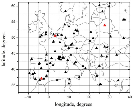
Figure 1.
Location of the Aerosol Robotic Network (AERONET) sites (black triangles) considered in the assimilation scheme. Red triangles are the sites chosen for validation.
Because the model AOD uncertainty [23] is significantly larger than the AERONET AOD uncertainty, we assumed the AERONET AOD uncertainty to be negligible. Prior to the implementation of the STOI, we compared GEOS-Chem simulated AOD with AERONET observations. The comparison revealed a bias of −0.032 for 440 nm, −0.025 for 675 nm, and −0.024 for 870 nm. Moreover, it was revealed that the dispersion of AERONET AOD is significantly larger than the dispersion of GEOS-Chem-simulated AOD for each wavelength. To correct the discrepancy, we used linear regression. After that, the STOI method was applied using the corrected AOD values simulated by GEOS-Chem.
To implement STOI we should know the spatial and temporal correlation functions. We obtained error statistics using observations from AERONET European stations, and simulations by a chemical transport model GEOS-Chem. We calculated spatial correlation coefficients of the model-minus-observation pairs of AOD at two spatial locations depending on the distance between them. We determined temporal correlation coefficients of the model-minus-observation pairs of AOD at two temporal locations, depending on the temporal interval between them. We constructed the correlations curves by fitting to the points presenting the obtained correlation coefficients. After that, we modeled the correlation curves by analytical functions. We chose exponential functions because they guarantee the positive definition of covariance matrices [27]. The exponential functions were chosen with argument kd, where d is the distance in kilometers or the time interval in days for the spatial or temporal correlation functions, respectively, and k is a fitting factor. The best fit was provided by k = 0.002 at 440 nm, 0.0025 at 675 nm, and 0.003 at 870 nm for the spatial correlation function, and k = 0.4 at 440 nm, 0.45 at 675 nm, and 0.5 at 870 nm for the temporal correlation function. The obtained spatial and temporal correlation curves are presented in Figure 2.
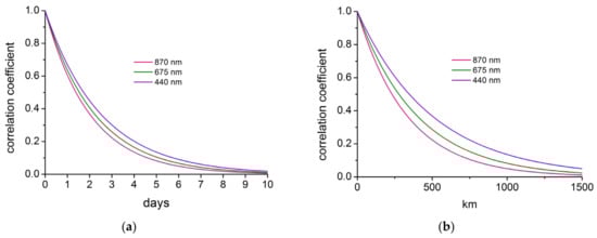
Figure 2.
(a) Temporal and (b) spatial correlation coefficients at 440 (violet line), 675 (green), and 870 (red) nm.
Figure 2 shows that the correlation coefficient value slightly decreases with an increase in the wavelength. A possible reason for such behavior is the larger contribution to AOD at longer wavelengths by coarse aerosol particles, which have higher spatial and temporal variability than fine particles.
We used the correlation functions to construct the covariance matrix of model errors. We calculated the weighting matrix for every spatial-temporal grid cell, using Equation (2), with a temporal resolution of 1 day. According to OI, not all available observations were considered: only those lying near the point being updated. We chose the number of observations using empirical selection criteria. Some tuning of numerical parameters is a common practice in data assimilation [34]. We accepted the spatial correlation length of 850 km and the temporal correlation length of 5 days. These are the intervals where the correlation coefficient is equal to about 0.1. We assumed the separation of spatial and temporal correlations. We calculated spatial-temporal correlation coefficients for a given distance and time interval as a product of corresponding spatial and temporal correlation coefficients. If the resulting correlation coefficient turned out to be less than 0.08, it was considered zero. The covariance matrix of observational errors was assumed as a zero matrix. The estimates of AOD at every grid cell were determined from Equation (1).
3. Results
Using the STOI method, we estimated the distribution of the daily averaged AOD in Europe for 2015–2016. Figure 3 shows an example of the distribution of daily mean AOD at 870 nm before STOI (modeled by GEOS-Chem) and after STOI (estimated using assimilated AERONET observations) for 17 July 2015. We chose the date arbitrarily. The example illustrates the change in AOD distribution over Europe after applying STOI.
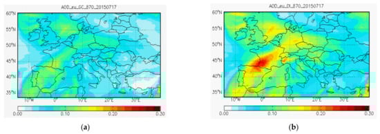
Figure 3.
Distribution of daily mean AOD at 870 nm (a) modeled by GEOS-Chem and (b) estimated with the use of assimilated AERONET observations for 17 July 2015.
Figure 3 shows only individual cases and cannot be used for generalized conclusions. The statistical processing of obtained estimates will be performed in the future. However, Figure 3 confirms that the GEOS-Chem simulation underestimates AOD in general.
To validate the results, we compared the daily mean AOD estimated by STOI with independent AERONET observations. The AERONET sites Granada, Lille, and Minsk (see Figure 1, red triangles) were excluded from the assimilation scheme, and STOI for July and November 2015 was performed using data from 83 remaining sites. July is the month with the most AERONET observations. The number of observations is small in November in the northern part of Europe because of many cloudy days. We considered only days with Level 2.0 observations. At the Granada site, there were 29 days with observations in July 2015 and 28 days in November 2015. There were 21 days at the Lille site and 31 days at the Minsk site in July 2015, and only 6 days at Lille and Minsk sites in November 2015.
The AERONET Granada, Lille, and Minsk sites chosen for validation also differ in the number of neighboring AERONET sites and the distance between sites. Minsk is located in the eastern European region, where observations are sparse. The location of AERONET sites in the Minsk region is shown in Figure 4a. Only six AERONET stations operated in 2015 within the correlation length for the Minsk site, and all of them are at a significant distance from this AERONET site.

Figure 4.
Location of the AERONET sites (black triangles) considered in the assimilation scheme for the Minsk region (a), Lille region (b), and Granada region (c). Red triangles are the sites chosen for validation.
In contrast with the Minsk site, there is a significant amount of AERONET sites close to the Granada and Lille sites. Nineteen AERONET sites were taken into account in the Lille region. The location of these sites is shown in Figure 4b. Twenty AERONET sites were considered in the Granada region. Their location is shown in Figure 4c.
We obtained estimates of daily mean AOD at each of the excluded sites for every day in November and July 2015. We calculated root-mean-square errors of the estimates using AOD observations at those sites when Level 2.0 observations existed, assuming a negligible error of the AERONET AOD observations. The root–mean–square errors (RMSE) of model-simulated AOD were calculated at the Granada, Lille, and Minsk sites. The comparison results are shown in Table 1 for July and Table 2 for November. In parentheses, the reduction in RMSE of the estimate after STOI is shown in tables.

Table 1.
Root-mean-square errors of the aerosol optical depth (AOD) calculated using GEOS-Chem and assimilated using spatial-temporal optimal interpolation (STOI) as compared to AOD observed by AERONET in July 2015.
Table 2.
Root-mean-square errors of the aerosol optical depth (AOD) calculated using GEOS-Chem and assimilated using spatial-temporal optimal interpolation (STOI) as compared to AOD observed by AERONET in November 2015.
4. Discussion and Conclusions
In this study, we presented a spatial-temporal optimal interpolation method for evaluating atmospheric aerosol load in locations where direct measurements on-site are unavailable. The observations in neighboring AERONET sites and model retrievals were linearly combined, accounting for their relative errors, to estimate the spatial and temporal distribution of AOD. The AOD values were calculated with the use of STOI to check the STOI method applicability. Results were compared with observations at Granada, Lille, and Minsk AERONET sites in July and November 2015.
In July, the RMSE of the estimate after STOI is significantly less than the RMSE of model-simulated AOD for every three sites at every three wavelengths. After averaging over three wavelengths (Table 1), the reduction in RMSE of the estimate after STOI in July is 68% for the Granada site, 45% for the Lille site, and 22% for the Minsk site. The best improvement among those three sites is achieved for Granada. This improvement is due to the presence of a number of AERONET stations located close to the Granada site, and the significant errors in the GEOS-Chem calculations for the Granada site during the period under consideration. A relatively poor improvement occurs for the Minsk site because of insufficient coverage of observations in the eastern European region. The dominant source of errors in assimilated AOD in this region arises from uncertainties in the model results.
In November, the RMSE of the estimate after STOI for Granada is comparable with that in July. However, the RMSE of modeled AOD was significantly lower in November 2015 than in July 2015. Accordingly, the reduction in RMSE is lower in November. For the Minsk site, the RMSE of both modeled and assimilated AOD is approximately the same in July and November. Averaged over three wavelengths, the reduction in RMSE of the estimate after STOI in November (Table 2) is 26% for the Granada site, and 18% for the Minsk site. For the Lille site, the percentage of STOI RMSE in November is negative: −19% on average, which is due to a perfect agreement between modeled and observed AOD for Lille in November, especially for the 870 nm wavelength. That is most likely a rare case.
In [43], we evaluated the correlation between the observed AOD and the modeled by GEOS-Chem AOD values, using statistics of observations at the 88 European AERONET sites for the 2015–2016 period. The correlation coefficients obtained in [43] were 0.60, 0.53, and 0.45 for wavelengths 440, 675, and 870 nm, respectively. Therefore, the discrepancy between observed and modeled values of AOD is usually significant.
Generally, the reduction of the RMSE averaged over two months, and three sites are about 25%. The result shows that STOI improves an estimate of AOD compared to model calculations. In the locations where the AERONET site density is high, STOI expectedly shows better improvements. In this paper, we assimilated AERONET data only. The satellite data assimilation will be considered using STOI in future work. Although the present study is focused on AOD only, the STOI technique can be applied to other aerosol properties and atmospheric species.
Author Contributions
Conceptualization, N.M., G.M. and A.C.; methodology, N.M. and A.B.; software, N.M. and A.B.; validation, N.M. and A.B.; investigation, N.M., A.B., G.M., and Y.Y.; resources, A.C. and G.M.; data curation, A.C., G.M., and A.M.; writing—original draft preparation, N.M.; writing—review and editing, G.M., A.C., A.B., A.M. and Y.Y.; visualization, N.M. and A.B.; supervision, N.M., G.M. and A.C.; project administration, N.M. and G.M.; funding acquisition, G.M. All authors have read and agreed to the published version of the manuscript.
Funding
This work was partly supported by the Belarusian Republican Foundation for Fundamental Research through the project F20UKA-017; by the College of Physics International Center of Future Science, Jilin University, China; by Ministry of Education and Science of Ukraine, through the projects BF/30-2021. The work was partly supported from the European Union’s Horizon 2020 research and innovation program under the Marie Skłodowska-Curie grant agreement No 778349, the research and innovation program under ACTRIS-2 grant agreement No 654109 and the European Commission Horizon 2020 Program that funded the ERA-PLANET/SMURBS project.
Institutional Review Board Statement
Not applicable.
Informed Consent Statement
Not applicable.
Data Availability Statement
AERONET data are freely available from https://aeronet.gsfc.nasa.gov (accessed on 1 November 2022). GEOS-Chem simulation and the STOI data generated in this work are freely available from http://scat.bas-net.by/~assimilation/(accessed on 1 November 2022).
Acknowledgments
We thank Brent Holben, Pawan Gupta, Elena Lind, and David Giles (NASA/GSFC) for managing the AERONET program and its sites. The high-quality AERONET/PHOTONS data provided by the CIMEL sun, sky, and lunar photometer calibration performed at the AERONET-EUROPE calibration center.
Conflicts of Interest
The authors declare no conflict of interest.
References
- Davidson, C.I.; Phalen, R.F.; Solomon, P.A. Airborne Particulate Matter and Human Health: A Review. Aerosol Sci. Technol. 2005, 39, 737–749. [Google Scholar] [CrossRef]
- Oh, H.-J.; Ma, Y.; Kim, J. Human Inhalation Exposure to Aerosol and Health Effect: Aerosol Monitoring and Modelling Regional Deposited Doses. Int. J. Environ. Res. Public Health 2020, 17, 1923. [Google Scholar] [CrossRef] [PubMed]
- Christodoulakis, J.; Varotsos, C.A.; Cracknell, A.P.; Kouremadas, G.A. The Deterioration of Materials as a Result of Air Pollution as Derived from Satellite and Ground Based Observations. Atmos. Environ. 2018, 185, 91–99. [Google Scholar] [CrossRef]
- Varotsos, C.; Tzanis, C.; Cracknell, A. The Enhanced Deterioration of the Cultural Heritage Monuments Due to Air Pollution. Environ. Sci. Pollut. Res. 2009, 16, 590–592. [Google Scholar] [CrossRef] [PubMed]
- IPCC. Climate Change 2022: Impacts, Adaptation, and Vulnerability—Contribution of Working Group II to the Sixth Assessment Report of the Intergovernmental Panel on Climate Change; Pörtner, H.-O., Roberts, D.C., Tignor, M., Poloczanska, E.S., Mintenbeck, K., Alegría, A., Craig, M., Langsdorf, S., Löschke, S., Möller, V., Eds.; Cambridge University Press: Cambridge, UK, 2022; Available online: https://www.ipcc.ch/report/ar6/wg2/ (accessed on 6 December 2022).
- Sayer, A.M. How Long is Too Long? Variogram Analysis of AERONET Data to Aid Aerosol Validation and Intercomparison Studies. Earth Space Sci. 2020, 7, e2020EA001290. [Google Scholar] [CrossRef]
- Li, J.; Kahn, R.A.; Wei, J.; Carlson, B.E.; Lacis, A.A.; Li, Z.; Li, X.; Dubovik, O.; Nakajima, T. Synergy of Satellite- and Ground-Based Aerosol Optical Depth Measurements Using an Ensemble Kalman Filter Approach. J. Geophys. Res. Atmos. 2020, 125, e2019JD031884. [Google Scholar] [CrossRef]
- Zang, Z.; You, W.; Ye, H.; Liang, Y.; Li, Y.; Wang, D.; Hu, Y.; Yan, P. 3DVAR Aerosol Data Assimilation and Evaluation Using Surface PM2.5, Himawari-8 AOD and CALIPSO Profile Observations in the North China. Remote Sens. 2022, 14, 4009. [Google Scholar] [CrossRef]
- Varotsos, C.A.; Efstathiou, M.N.; Cracknell, A.P. On the association of aerosol optical depth and total ozone fluctuations with recent earthquakes in Greece. Acta Geophys. 2017, 65, 659–665. [Google Scholar] [CrossRef]
- Holben, B.N.; Eck, T.F.; Slutsker, I.; Tanre, D.; Buis, J.P.; Setzer, A.; Vermote, E.; Reagan, J.A.; Kaufman, Y.J.; Nakajima, T.; et al. AERONET—A Federated Instrument Network and Data Archive for Aerosol Characterization. Remote Sens. Environ. 1998, 66, 1–16. [Google Scholar] [CrossRef]
- Sayer, A.M.; Hsu, N.C.; Bettenhausen, C.; Jeong, M.-J. Validation and Uncertainty Estimates for MODIS Collection 6 “Deep Blue” Aerosol Data. J. Geophys. Res. Atmos. 2013, 118, 7864–7872. [Google Scholar] [CrossRef]
- Wei, J.; Li, Z.; Peng, Y.; Sun, L. MODIS Collection 6.1 Aerosol Optical Depth Products over Land and Ocean: Validation and Comparison. Atmos. Environ. 2019, 201, 428–440. [Google Scholar] [CrossRef]
- Holben, B.N.; Kim, J.; Sano, I.; Mukai, S.; Eck, T.F.; Giles, D.M.; Schafer, J.S.; Sinyuk, A.; Slutsker, I.; Smirnov, A.; et al. An Overview of Mesoscale Aerosol Processes, Comparisons, and Validation Studies from DRAGON Networks. Atmos. Chem. Phys. 2018, 18, 655–671. [Google Scholar] [CrossRef]
- NASA; Goddard Space Flight Center; AERONET. Aerosol Robotic Network. Available online: https://aeronet.gsfc.nasa.gov/ (accessed on 1 November 2022).
- Dubovik, O.; King, M.D. A Flexible Inversion Algorithm for Retrieval of Aerosol Optical Properties from Sun and Sky Radiance Measurements. J. Geophys. Res. 2000, 105, 20673–20696. [Google Scholar] [CrossRef]
- Eck, T.F.; Holben, B.N.; Reid, J.S.; Dubovik, O.; Smirnov, A.; O’Neill, N.T.; Slutsker, I.; Kinne, S. Wavelength Dependence of the Optical Depth of Biomass Burning, Urban and Desert Dust Aerosols. J. Geophys. Res. 1999, 104, 31333–31349. [Google Scholar] [CrossRef]
- Holben, B.N.; Tanre, D.; Smirnov, A.; Eck, T.F.; Slutsker, I.; Abuhassan, N.; Newcomb, W.W.; Schafer, J.; Chatenet, B.; Lavenue, F.; et al. An Emerging Ground-Based Aerosol Climatology: Aerosol Optical Depth from AERONET. J. Geophys. Res. 2001, 106, 12067–12097. [Google Scholar] [CrossRef]
- Chin, M.; Ginoux, P.; Kinne, S.; Torres, O.; Holben, B.N.; Duncan, B.N.; Martin, R.V.; Logan, J.A.; Higurashi, A.; Nakajima, T. Tropospheric Aerosol Optical Thickness from the GOCART Model and Comparisons with Satellite and Sun Photometer Measurements. J. Atmos. Sci. 2002, 59, 461–483. [Google Scholar] [CrossRef]
- Morcrette, J.-J.; Boucher, O.; Jones, L.; Salmond, D.; Bechtold, P.; Beljaars, A.; Benedetti, A.; Bonet, A.; Kaiser, J.W.; Razinger, M.; et al. Aerosol Analysis and Forecast in the European Centrefor Medium-Range Weather Forecasts Integrated Forecast System: Forward Modeling. J. Geophys. Res. 2009, 114, D06206. [Google Scholar] [CrossRef]
- Carnevale, C.; Finzi, G.; Mannarini, G.; Pisoni, E.; Volta, M. Comparing Mesoscale Chemistry-Transport Model and Remote-Sensed Aerosol Optical Depth. Atmos. Environ. 2011, 45, 289–295. [Google Scholar] [CrossRef][Green Version]
- Meier, J.; Tegen, I.; Mattis, I.; Wolke, R.; Alados Arboledas, L.; Apituley, A.; Balis, D.; Barnaba, F.; Chaikovsky, A.; Sicard, M.; et al. A Regional Model of European Aerosol Transport: Evaluation with Sun Photometer, Lidar and Air Quality Data. Atmos. Environ. 2012, 47, 519–532. [Google Scholar] [CrossRef]
- Li, S.; Yu, C.; Chen, L.; Tao, J.; Letu, H.; Ge, W.; Si, Y.; Liu, Y. Inter-Comparison of Model-Simulated and Satellite-Retrieved Componential Aerosol Optical Depths in China. Atmos. Environ. 2016, 141, 320–332. [Google Scholar] [CrossRef]
- Li, S.; Garay, M.J.; Chen, L.; Rees, E.; Liu, Y. Comparison of GEOS-Chem Aerosol Optical Depth with AERONET and MISR Data over the Contiguous United States. J. Geophys. Res. 2013, 118, 11228–11241. [Google Scholar] [CrossRef]
- Daley, R. Atmospheric Data Analysis; Cambridge University Press: Cambridge, UK, 1991. [Google Scholar]
- Ghil, M.; Malanotte-Rizzoli, P. Data Assimilation in Meteorology and Oceanogrphy. Adv. Geophys. 1991, 33, 141–266. [Google Scholar] [CrossRef]
- Lahoz, W.A.; Schneider, P. Data Assimilation: Making Sense of Earth Observation. Front. Environ. Sci. 2014, 2, 16. [Google Scholar] [CrossRef]
- Gandin, L.S. Objective Analysis of Meteorological Fields; Gidrometeorol. Izd.: Leningrad, Russia, 1963. [Google Scholar]
- Lorenc, A.C. A Global Three-Dimensional Multivariate Statistical Analysis Scheme. Mon. Weather Rev. 1981, 109, 701–721. [Google Scholar] [CrossRef]
- Collins, W.D.; Rasch, P.J.; Eaton, B.E.; Khattatov, B.V.; Lamarque, J.-F.; Zender, C.S. Simulating Aerosols Using a Chemical Transport Model with Assimilation of Satellite Aerosol Retrievals: Methodology for INDOEX. J. Geophys. Res. Atmos. 2001, 106, 7313–7336. [Google Scholar] [CrossRef]
- Kalman, R.E. A New Approach to Linear Filtering and Prediction Problems. J. Basic Eng. 1960, 82, 35–45. [Google Scholar] [CrossRef]
- Kalnay, E. Atmospheric Modeling, Data Assimilation and Predictability; Cambridge University Press: Cambridge, UK, 2002. [Google Scholar]
- Evensen, G. Data Assimilation: The Ensemble Kalman Filter; Springer: Berlin/Heidelberg, Germany, 2009. [Google Scholar]
- Sekiyama, T.T.; Tanaka, T.Y.; Shimizu, A.; Miyoshi, T. Data Assimilation of CALIPSO Aerosol Observations. Atmos. Chem. Phys. 2010, 10, 39–49. [Google Scholar] [CrossRef]
- Schutgens, N.A.J.; Miyoshi, T.; Takemura, T.; Nakajima, T. Applying an Ensemble Kalman Filter to the Assimilation of AERONET Observations in a Global Aerosol Transport Model. Atmos. Chem. Phys. 2010, 10, 2561–2576. [Google Scholar] [CrossRef]
- Sasaki, Y. An Objective Analysis Based on the Variational Method. J. Meteorol. Soc. Jpn. 1958, 36, 77–88. [Google Scholar] [CrossRef]
- Talagrand, O. A Study on the Dynamics of Four-Dimensional Data Assimilation. Tellus 1981, 33, 43–60. [Google Scholar] [CrossRef]
- Fisher, M.; Lary, D.J. Lagrangian Four-Dimensional Variational Data Assimilation of Chemical Species. Q. J. R. Meteorol. Soc. 1995, 121, 1681–1704. [Google Scholar] [CrossRef]
- Benedetti, A.; Morcrette, J.-J.; Boucher, O.; Dethof, A.; Engelen, R.J.; Fisher, M.; Flentje, H.; Huneeus, N.; Jones, L.; Kaiser, J.W.; et al. Aerosol Analysis and Forecast in the European Centre for Medium-Range Weather Forecasts Integrated Forecast System: 2. Data assimilation. J. Geophys. Res. 2009, 114, D13205. [Google Scholar] [CrossRef]
- Tombette, M.; Mallet, V.; Sportisse, B. PM10 Data Assimilation over Europe with the Optimal Interpolation Method. Atmos. Chem. Phys. 2009, 9, 57–70. [Google Scholar] [CrossRef]
- Lorenc, A.C. Analysis Methods for Numerical Weather Prediction. Q. J. R. Meteorol. Soc. 1986, 112, 1177–1194. [Google Scholar] [CrossRef]
- Sentchev, A.; Yaremchuk, M. Monitoring Tidal Currents with a Towed ADCP System. Ocean Dyn. 2016, 6, 119–132. [Google Scholar] [CrossRef]
- Stanev, E.V.; Ziemer, F.; Schulz-Stellenfleth, J.; Seemann, J.; Staneva, J.; Gurgel, K.-W. Blending Surface Currents from HF Radar Observations and Numerical Modeling: Tidal Hindcasts and Forecasts. J. Atmos. Ocean. Technol. 2015, 32, 256–281. [Google Scholar] [CrossRef]
- Miatselskaya, N.S.; Bril, A.I.; Chaikovsky, A.P.; Yukhymchuk, Y.Y.; Milinevski, G.P.; Simon, A.A. Optimal Interpolation of AERONET Radiometric Network Observations for the Evaluation of the Aerosol Optical Thickness Distribution in the Eastern European Region. J. Appl. Spectrosc. 2022, 89, 296–302. [Google Scholar] [CrossRef]
- Bey, I.; Jacob, D.J.; Yantosca, R.M.; Logan, J.A.; Field, B.D.; Fiore, A.M.; Li, Q.; Liu, H.Y.; Mickley, L.J.; Schultz, M.G. Global Modeling of Tropospheric Chemistry with Assimilated Meteorology: Model Description and Evaluation. J. Geophys. Res. 2001, 106, 23073–23096. [Google Scholar] [CrossRef]
- GEOS-Chem. Available online: https://geos-chem.seas.harvard.edu/ (accessed on 1 November 2022).
- Bovchaliuk, V.; Bovchaliuk, A.; Milinevsky, G.; Danylevsky, V.; Sosonkin, M.; Goloub, P. Aerosol Microtops II Sunphotometer Observations over Ukraine. Adv. Astron. Space Phys. 2013, 3, 46–52. [Google Scholar]
- Cimel Sunphotometer (NASA AERONET). Available online: https://appalair.appstate.edu/aerosol-research-program/nasa-aeronet-data (accessed on 10 December 2022).
- Giles, D.M.; Sinyuk, A.; Sorokin, M.G.; Schafer, J.S.; Smirnov, A.; Slutsker, I.; Eck, T.F.; Holben, B.N.; Lewis, J.R.; Campbell, J.R.; et al. Advancements in the Aerosol Robotic Network (AERONET) Version 3 Database—Automated Near-Real-Time Quality Control Algorithm with Improved Cloud Screening for Sun Photometer Aerosol Optical Depth (AOD) Measurements. Atmos. Meas. Tech. 2019, 12, 169–209. [Google Scholar] [CrossRef]
- NASA; Goddard Space Flight Center; Global Modeling and Assimilation Office; GEOS Systems. Available online: https://gmao.gsfc.nasa.gov/GEOS_systems/ (accessed on 1 November 2022).
- Lin, S.-J.; Rood, R.B. Multidimensional Flux Form Semi-Lagrangian Transport Schemes. Mon. Weather Rev. 1996, 124, 2046–2070. [Google Scholar] [CrossRef]
- Park, R.J.; Jacob, D.J.; Field, B.D.; Yantosca, R.M.; Chin, M. Natural and Transboundary Pollution Influences on Sulfate-Nitrate-Ammonium Aerosols in the United States: Implications for Policy. J. Geophys. Res. 2004, 109, D15204. [Google Scholar] [CrossRef]
- Keller, C.A.; Long, M.S.; Yantosca, R.M.; Da Silva, A.M.; Pawson, S.; Jacob, D.J. HEMCO v1.0: A Versatile, ESMF-Compliant Component for Calculating Emissions in Atmospheric Models. Geosci. Model Dev. 2014, 7, 1409–1417. [Google Scholar] [CrossRef]
- Community Emissions Data System (CEDS). Available online: https://data.pnnl.gov/group/nodes/project/13463 (accessed on 10 December 2022).
- Hoesly, R.M.; Smith, S.J.; Feng, L.; Klimont, Z.; Janssens-Maenhout, G.; Pitkanen, T.; Seibert, J.J.; Vu, L.; Andres, R.J.; Bolt, R.M.; et al. Historical (1750–2014) Anthropogenic Emissions of Reactive Gases and Aerosols from the Community Emissions Data System (CEDS). Geosci. Model Dev. 2018, 11, 369–408. [Google Scholar] [CrossRef]
- Simone, N.W.; Stettler, M.E.J.; Barrett, S.R.H. Rapid Estimation of Global Civil Aviation Emissions with Uncertainty Quantification. Transp. Res. D Transp. Environ. 2013, 25, 33–41. [Google Scholar] [CrossRef]
- Global Fire Emissions Database. Available online: https://www.globalfiredata.org/ (accessed on 10 December 2022).
- Fairlie, T.D.; Jacob, D.J.; Park, R.J. The Impact of Transpacific Transport of Mineral Dust in the United States. Atmos. Environ. 2007, 41, 1251–1266. [Google Scholar] [CrossRef]
- Murray, L.T.; Jacob, D.J.; Logan, J.A.; Hudman, R.C.; Koshak, W.J. Optimized Regional and Interannual Variability of Lightning in a Global Chemical Transport Model Constrained by LIS/OTD Satellite Data. J. Geophus. Res. Atmos. 2012, 117, D20307. [Google Scholar] [CrossRef]
- Guenther, A.B.; Jiang, X.; Heald, C.L.; Sakulyanontvittaya, T.; Duhl, T.; Emmons, L.K.; Wang, X. The Model of Emissions of Gases and Aerosols from Nature Version 2.1 (MEGAN2.1): An Extended and Updated Framework for Modeling Biogenic Emissions. Geosci. Model Dev. 2012, 5, 1471–1492. [Google Scholar] [CrossRef]
- Hudman, R.C.; Moore, N.E.; Martin, R.V.; Russell, A.R.; Mebust, A.K.; Valin, L.C.; Cohen, R.C. A Mechanistic Model of Global Soil Nitric Oxide Emissions: Implementation and Space Based-Constraints. Atm. Chem. Phys. 2012, 12, 7779–7795. [Google Scholar] [CrossRef]
- Jaeglé, L.; Quinn, P.K.; Bates, T.; Alexander, B.; Lin, J.-T. Global Distribution of Sea Salt Aerosols: New Constraints from In Situ and Remote Sensing Observations. Atmos. Chem. Phys. 2011, 11, 3137–3157. [Google Scholar] [CrossRef]
- Van Donkelaar, A.; Martin, R.V.; Brauer, M.; Kahn, R.; Levy, R.; Verduzco, C.; Villeneuve, P.J. Global Estimates of Ambient Fine Particulate Matter Concentrations from Satellite-Based Aerosol Optical Depth: Development and Application. Environ. Health Perspect. 2010, 118, 847–855. [Google Scholar] [CrossRef]
- Van Donkelaar, A.; Martin, R.V.; Brauer, M.; Boys, B.L. Use of Satellite Observations for Long-Term Exposure Assessment of Global Concentrations of Fine Particulate Matter. Environ. Health Perspect. 2015, 123, 135–143. [Google Scholar] [CrossRef]
- Milinevsky, G.; Miatselskaya, N.; Grytsai, A.; Danylevsky, V.; Bril, A.; Chaikovsky, A.; Yukhymchuk, Y.; Wang, Y.; Liptuga, A.; Kyslyi, V.; et al. Atmospheric Aerosol Distribution in 2016–2017 over the Eastern European Region Based on the GEOS-Chem Model. Atmosphere 2020, 11, 722. [Google Scholar] [CrossRef]
- Latimer, R.N.C.; Martin, R.V. Interpretation of Measured Aerosol Mass Scattering Efficiency over North America Using a Chemical Transport Model. Atmos. Chem. Phys. 2019, 19, 2635–2653. [Google Scholar] [CrossRef]
- Ridley, D.A.; Heald, C.L.; Ford, B. North African Dust Export and Deposition: A Satellite and Model Perspective. J. Geophys. Res. 2012, 117, D02202. [Google Scholar] [CrossRef]
- Wang, Y.X.; Mcelroy, M.B.; Jacob, D.J.; Yantosca, R.M. A Nested Grid Formulation for Chemical Transport over Asia: Applications to CO. J. Geophys. Res. Atmos. 2004, 109, D22307. [Google Scholar] [CrossRef]
Disclaimer/Publisher’s Note: The statements, opinions and data contained in all publications are solely those of the individual author(s) and contributor(s) and not of MDPI and/or the editor(s). MDPI and/or the editor(s) disclaim responsibility for any injury to people or property resulting from any ideas, methods, instructions or products referred to in the content. |
© 2022 by the authors. Licensee MDPI, Basel, Switzerland. This article is an open access article distributed under the terms and conditions of the Creative Commons Attribution (CC BY) license (https://creativecommons.org/licenses/by/4.0/).