Forecasting PM₁₀ Concentrations in the Caribbean Area Using Machine Learning Models

Abstract

In the Caribbean basin, particulate matter lower or equal to 10 μm in diameter (PM₁₀) has a huge impact on human mortality and morbidity due to the African dust. For the first time in this geographical area, the theoretical framework of artificial intelligence is applied to forecast PM₁₀ concentrations. The aim of this study is to forecast PM₁₀ concentrations using six machine learning (ML) models: support vector regression (SVR), k-nearest neighbor regression (kNN), random forest regression (RFR), gradient boosting regression (GBR), Tweedie regression (TR), and Bayesian ridge regression (BRR). Overall, with MBE_max = −2.8139, the results showed that all the models tend to slightly underestimate PM₁₀ empirical data. GBR is the model that gives the best performance (r = 0.7831, R² = 0.6132, MAE = 6.8479, RMSE = 10.4400, and IOA = 0.7368). By comparing our results to other PM₁₀ ML studies in megacities, we found similar performance using only three input variables, whereas previous studies use many input variables with Artificial Neural Network (ANN) models. All these results showed the features of PM₁₀ concentrations in the Caribbean area.

1. Introduction

Due to climate change, the frequency and intensity of natural hazards have increased over the past century [1]. In the Caribbean basin, this results in an increase in extreme sand haze events [2,3]. Sand mists have a major health impact on the Caribbean population [4]. The African dust is associated with many cardiovascular and respiratory diseases, prematurity, and a series of infectious diseases [5,6,7,8,9].

To reach the Caribbean area, desert dust travels in a hot and dry layer above the Atlantic Ocean at an altitude between 1500 and 5000 m, i.e., the Saharan air layer (SAL) [10,11,12]. Due to the activation of dust sources in Africa, there is a seasonality in desert dust behavior with a high dust season which typically goes from May to September and a low season from October to April [13,14,15]. The particles from these dust outbreaks are found in the atmospheric boundary layer (ABL) mainly through dry and wet deposition [16]. Recent studies have shown that air temperature and rainfall are the two parameters that have a significant impact on the deposition of particles lower or equal to 10 μm in diameter ($P{M}_{10}$). Indeed, there is bidirectional causality between the $P{M}_{10}$ and the temperature [17], while the causality between the $P{M}_{10}$ and the rainfall is unidirectional [18]. Thus, during the high dust season, the high $P{M}_{10}$ concentrations increase air temperature values (greenhouse effect) [19,20] while during the low dust season, the lower air temperatures enhance the $P{M}_{10}$ dry deposition velocity, as the thermal convection of the soil is less significant [21,22]. Regarding the interaction between the $P{M}_{10}$ and the rainfall, $P{M}_{10}$ are particles too large to serve as condensation nuclei [23], while the rainfall induces the $P{M}_{10}$ wet scavenging process [18,24], i.e., the transfer of particles from the mixing layer to the surface layer.

In a complex environment such as the atmosphere, there are many interactions between the parameters [25]. To forecast $P{M}_{10}$ concentrations in the ABL, it is, therefore, necessary to take into account several variables simultaneously. Traditionally, deterministic methods and statistical modeling are widely used to forecast $PM$ [14,26,27,28,29]. Even though these approaches sometimes have high validity for prediction, many studies have shown that these methods cannot correctly simulate data in a complex environment [30,31,32,33].

To overcome these drawbacks, machine learning (ML) methods have been introduced [34]. The aim of this framework is to find optimized algorithms based on computational statistics [35]. Classically, ML methods allow researchers to automatically find the relevant input variables and develop an optimal model structure within the limits of the concept of the applied method [36]. Nevertheless, each method has a selective superiority. In other words, a model that is suitable for one task may not be adequate for another [36]. This is the reason why it is necessary to use several methods to find the one that provides the best prediction [37]. In the literature, many studies in Europe, China, Korea, and the United States have already used ML methods to forecast $P{M}_{10}$ concentrations [32,35,36,38,39,40,41,42,43,44,45,46]. To our knowledge, no study has yet used ML models to forecast $P{M}_{10}$ concentrations in the Caribbean area. Unlike other studies that use many predictor variables, here, only air temperature and rainfall mentioned earlier were used to carry out this study.

2. Data Presentation

In this study, we used the daily averages of $P{M}_{10}$ concentrations measured from 2005 to 2012 at the urban station of Pointe-à-Pitre (16.24° N–61.54° W) located in the center of Guadeloupe archipelago (16.25° N–61.58° W), a French West Indies island in the Caribbean area [20]. A quarter of the population lives in this area where the topography is nearly flat [47], and concrete buildings do not exceed four floors [48]. The main industrial area and the largest open landfill on the island are also in the same location [49].

The details on the sensors of the Pointe-à-Pitre monitoring station are described in Plocoste et al. [50]. The $P{M}_{10}$ data were collected by Gwad’Air Agency (https://www.gwadair.fr/, accessed on 30 November 2022), which manages the Guadeloupe air quality network. To complement $P{M}_{10}$ data, the study also used the daily averages of air temperature (T) and the daily sum of rainfall ($RR$) from the French center for weather forecast, Météo-France (https://meteofrance.gp/fr, accessed on 30 November 2022), located at the international airport of Pôle Caraïbes in the suburban area of Abymes (16.26° N–61.51° W). Both time series were previously pre-processed. Hence, no anomalous data were found due to the validation process performed by Gwad’Air and Météo France. It is important to emphasize that $P{M}_{10}$ and meteorological measurements were made under the same atmospheric conditions, i.e., in the insular continental regime of the island [51]. Figure 1 shows the simultaneous sequences between $P{M}_{10}$, T, and $RR$ time series. At first glance, one can notice that each time series seems to follow the same behavior.

3. Theoretical Framework

3.1. Machine Learning Models

In the literature, there are several machine learning forecasting techniques for time series. In this study, six robust methods were used: support vector regression, k-nearest neighbor regression, random forest regression, gradient boosting regression, Tweedie regression, and Bayesian ridge regression. All these methods were developed in the scikit-learn library in Python. In this theoretical framework, these methods are introduced, and the main parameters to perform the forecasting are presented.

3.1.1. Support Vector Regression (SVR)

SVR is a supervised statistical learning algorithm for regression problems [52]. It aims to reduce the error by determining the hyperplane and minimizing the range between the predicted and the observed values by solving Equation (2) of the model [53]. The main SVR parameters are C and $\gamma$ which are associated with the kernel function. Firstly, C is determined by minimizing the following regression equation:

$$\frac{1}{2}{\left|\right|w\left|\right|}^2+C\sum _{i=1}^N{ϵ}_i+{ϵ}_i^{*}\to min$$

(1)

where w is the sum of weights that regularize this model, and C is the constant parameter to define (C > 0), which determines the trade-off between the hyperplane and estimation error. C depends on the input data; if C is large, the margin of the estimated error will be small and thus avoids overfitting, whereas if C is small, the margin between the hyperplane and the estimated error will be large, which means many prediction errors. $ϵ-{ϵ}^{*}$ represents the slack variables defining the distance between the hyperplane margin and the prediction.

The other parameter is determined by solving Equation (1) with Lagrange multipliers $({\alpha }_i-{\alpha }_i^{*})$ as [54,55]:

$$f\left(x\right)=\sum _{i=1}^l({\alpha }_i-{\alpha }_i^{*})k(x_i-x_i^{*})+b$$

(2)

where $k(x_i-x_i^{*})$ is the kernel function according to the training values, and b is the bias terms.

There exist many kernel functions to solve Equation (2). Here, the radial basis function (RBF) was chosen, as it seems to be the best-adapted function in time series [56]:

$$k(x_i-x_i^{*})=exp\left(-\gamma \left|\right|x_i-x_i^{*}{\left|\right|}^2\right)$$

(3)

where $\gamma$ is the constant parameter to determine the region of similarity. $\gamma$ is the last important parameter of this model. If $\gamma$ is large, the exponential function is close to 0, which means the region of similarity is small. Conversely, if $\gamma$ is small, the similarity region is large.

Using the RBF kernel with a good trade-off between C and $\gamma$ parameters means a large C and a small $\gamma$ should give the best model performance.

3.1.2. k-Nearest Neighbor Regression (kNN)

The kNN algorithm is a popular supervised ML method [57]. This algorithm is based on the knowledge of neighboring values to make a prediction. Classically, kNN algorithms are frequently used in time series forecasting due to their simplicity and intuitiveness [58]. To build a kNN model, the entire training data are considered to find the k values closest to data prediction.

In order to perform this model, a metric distance associated with a decision tree was used. There are several distances, but the best known and widely used for regression models is the Euclidean distance:

$$Euclideandistance=\sqrt{\sum _i^N}{(x_i-x_i^{*})}^2$$

(4)

where $x_i-x_i^{*}$ represents the difference between two points for N data. Thus, the predicted values are the mean (or median) of the k-output neighbors found.

It is difficult to directly find the best k to use in this algorithm. The best approach is to try different k values and see which k gives the best result. In other words, many iterations are performed to find the best k.

3.1.3. Random Forest Regression (RFR)

The RF algorithm developed by Breiman [59] is one of the most used ML methods to build prediction models. This model is composed of predictor trees, and each tree depends on the values of a random vector sampled independently and with the same distribution for all the trees in the forest. The shape of these trees is very important for model performance. Some important parameters considered for RF accuracy include the following:

• The number of trees in the forest: the more trees we have, the more accurate the model is. Nevertheless, this increases the time of RF computations;
• Max depth: the depth of each tree;
• Bootstrap: this technique is used in RF to improve the robustness of forecasting. Bootstrap is performed to reduce the variance in each training sample of a tree. Consequently, this avoids overfitting [60];
• Criterion: a function to measure the quality of a split. Here, the squared error was chosen in order to minimize the mean-squared error of the current tree given the split.

With these main parameters, each tree has the same distribution and predicts in the same way. Hence, the final prediction is the average of several tree predictions.

3.1.4. Gradient Boosting Regression (GBR)

GB machines are a family of powerful machine learning techniques that have shown good results in a wide range of practical applications [61]. Boosting is a method that combines multiple base models to build a cluster, the performance of which can be significantly better than any other base model [62].

For this purpose, GBR builds the model in steps using several decision trees with weak performance and combines them to build an increasingly efficient model. For each step, GBR solves the following equation:

$$f_m\left(x\right)=f_{m-1}\left(x\right)+v_m{h}_m\left(x\right)$$

(5)

where $f_{m-1}\left(x\right)$ is the previous prediction, $v_m$ is the learning rate that reduces the effect of each previous tree on the next tree (usually $0<v_m<1$), and $h_m\left(x\right)$ is the function made on residuals composed of a loss function.

For continuous data, the loss function is minimized with the following equation:

$$L=\frac{1}{n}\sum _{i=0}^n{\left(y_i-{\widehat{y}}_i\right)}^2$$

(6)

where $y_i$ is the training data, ${\widehat{y}}_i$ is the data to predict, and n is the feature number.

GBR has many benefits such as the robustness of outliers in the output space using robust loss functions. It shows a high predictive power and natural processing, but its computational cost is significant for large databases.

3.1.5. Tweedie Regression (TR)

TR is a technique that belongs to the exponential dispersion model family and is defined as a generalized linear model. This method is simple and accurate with meteorological data of distribution Gamma [63]. Tweedie is defined by the following equation with a variant form:

$$Var\left(Y\right)=\phi {\mu }^{\xi }$$

(7)

where $\mu$ is the mean of the distribution, $\phi$ is the dispersion parameter, and $\xi$ is the Tweedie parameter. $\xi$ is chosen according to data distribution. The best-known distributions are normal ($\xi$ = 0), Poisson ($\xi$ = 1), Gamma ($\xi$ = 2). and Inverse Gaussian ($\xi$ = 3).

According to Smyth [63], for time series as meteorological data, we need to use Tweedie assuming that the distribution is Poisson–Gamma ($1<\xi <2$).

3.1.6. Bayesian Ridge Regression (BRR)

BRR is a probabilistic model like Bayesian linear regression with a ridge parameter. The aim of this model is to minimize the squared error between the predicted and actual observations by adding a ridge parameter ${a\left|\right|w\left|\right|}^2$, which is the sum of the squared weights [64]:

$${a\left|\right|w\left|\right|}^2+\sum _{i=1}^l{(y_i-x_i·w)}^2\to min$$

(8)

where $y_i$ is the outcome variable, $x_i$ is the parameter variable, w is the sum of the weights, and a is the accuracy of the weights ($0<a<1$).

3.2. Evaluation of Forecast Performance

ML forecast performance can be evaluated using classical statistical performance indicators such as Pearson’s correlation coefficient (r), coefficient of determination ($R^2$), mean absolute error ($MAE$), mean bias error ($MBE$), root mean square error ($RMSE$) and index of agreement ($IOA$). r measures how strong the linear relationship is between the observed and predicted values, $R^2$ represents the proportion of variance explained by the model, and $IOA$ describes how close the observed and predicted values are. The model performance is significant when their values are close to 1. $MAE$, $MBE$, and $RMSE$ were applied to quantify the forecast errors, which should be close to zero. r, $R^2$, $MAE$, $MBE$, $RMSE$, and $IOA$ were computed as follows [41,65,66,67]:

$$r=\frac{{\sum }_{i=1}^N(\widetilde{P_i}-\overline{P})(O_i-\overline{O})}{\sqrt{{\sum }_{i=1}^N{(\widetilde{P_i}-\overline{P})}^2\times {\sum }_{i=1}^N{(O_i-\overline{O})}^2}}$$

(9)

$$R^2=1-\frac{{\sum }_{i=1}^N{(\widetilde{P_i}-O_i)}^2}{{\sum }_{i=1}^N{(O_i-\overline{O})}^2}$$

(10)

$$MAE=\frac{1}{N}\sum _{i=1}^N\left|(\widetilde{P_i}-O_i)\right|$$

(11)

$$MBE=\frac{1}{N}\sum _{i=1}^N(\widetilde{P_i}-O_i)$$

(12)

$$RMSE=\sqrt{\frac{1}{N}\sum _{i=1}^N{(\widetilde{P_i}-O_i)}^2}$$

(13)

$$IOA=1-\left(\frac{{\sum }_{i=1}^N{(\widetilde{P_i}-O_i)}^2}{{\sum }_{i=1}^N\left(\right|\widetilde{P_i}-\overline{O}|+|O_i-\overline{O}{\left|\right)}^2}\right)$$

(14)

where $\widetilde{P_i}$ is the predicted value, $O_i$ is the observed value, $\overline{P}$ is the predicted average value, and $\overline{O}$ is the observed average value.

4. Results and Discussion

4.1. Data Analysis

To investigate the behavior of $P{M}_{10}$, T, and $RR$ in the Caribbean area, descriptive statistics were first computed. Thus, the mean ($\overline{M}$), standard deviation ($\sigma$), skewness (S), and kurtosis (K) were chosen to analyze the trend, fluctuation, asymmetry, and intermittency of the studied variables, respectively [68]. Highly intermittent time series have higher kurtosis values [69].

Table 1. The arithmetic mean ($\overline{M}$), standard deviation ($\sigma$), skewness (S), and kurtosis (K) of $P{M}_{10}$, T, and $RR$ by year. For $P{M}_{10}$-T-$RR$, $\overline{M}$ and $\sigma$ are, respectively, in μg/m³-°C-mm, while N is the sample size.

	${\mathit{PM}}_{10}$				T				$\mathit{RR}$
Year	$\overline{\mathit{M}}$	$\mathit{\sigma }$	$\mathit{S}$	$\mathit{K}$	$\overline{\mathit{M}}$	$\mathit{\sigma }$	$\mathit{S}$	$\mathit{K}$	$\overline{\mathit{M}}$	$\mathit{\sigma }$	$\mathit{S}$	$\mathit{K}$
2005 (N = 354)	27.3	15.3	2.3	9.1	26.2	1.6	−0.5	2.5	5.4	11.0	3.9	22.3
2006 (N = 358)	27.8	16.6	1.7	5.5	26.1	1.5	−0.3	2.1	4.1	7.7	3.3	15.4
2007 (N = 357)	27.8	17.5	2.5	12.8	26.3	1.4	−0.2	2.1	2.8	5.9	4.2	25.5
2008 (N = 355)	24.9	13.1	3.2	18.3	25.7	1.6	−0.2	2.1	4.4	8.5	3.4	16.2
2009 (N = 365)	24.8	14.5	3.0	14.9	26.1	1.5	−0.1	1.9	3.5	7.7	5.8	47.8
2010 (N = 354)	27.5	19.7	2.9	15.0	26.7	1.3	−0.2	2.2	4.9	11.1	5.3	45.1
2011 (N = 352)	24.4	13.8	2.0	7.3	25.9	1.5	−0.1	2.1	5.8	12.9	5.6	46.5
2012 (N = 351)	28.4	17.2	1.3	3.9	26.2	1.5	−0.4	2.2	3.9	8.7	4.6	29.4

presents the statistical parameters for $P{M}_{10}$, T, and $RR$ by year.

For $\overline{M}$-$\sigma$-S-K, one can notice that T values are more homogeneous than $P{M}_{10}$ and $RR$. This is due to the fact that T strongly depends on the annual cycle of the earth around the sun [70], while the highest values of $P{M}_{10}$ and $RR$ mainly depend on the African dust season [12] and the hurricane season [71]. In other words, T variation is strongly linked to planetary scale phenomena, while $P{M}_{10}$ and $RR$ are influenced by the synoptic scale phenomena. This is the reason why the distribution of T values seems to correspond to a Gaussian law (S = 0 and K = 3). The annual inter-variability of $K_{P{M}_{10}}$ and $K_{RR}$ shows that, from one year to another, the intensity and duration of sand haze and rainfall can vary significantly [72,73]. Even if $P{M}_{10}$ and $RR$ values are more heterogeneous than those of T, one can observe that $\overline{M}$-$\sigma$-S are of the same order of magnitude between the years. Thus, there is an inter-annual stationarity for T, $P{M}_{10}$, and $RR$. All these results show that the required statistical conditions were met when setting up the statistical models.

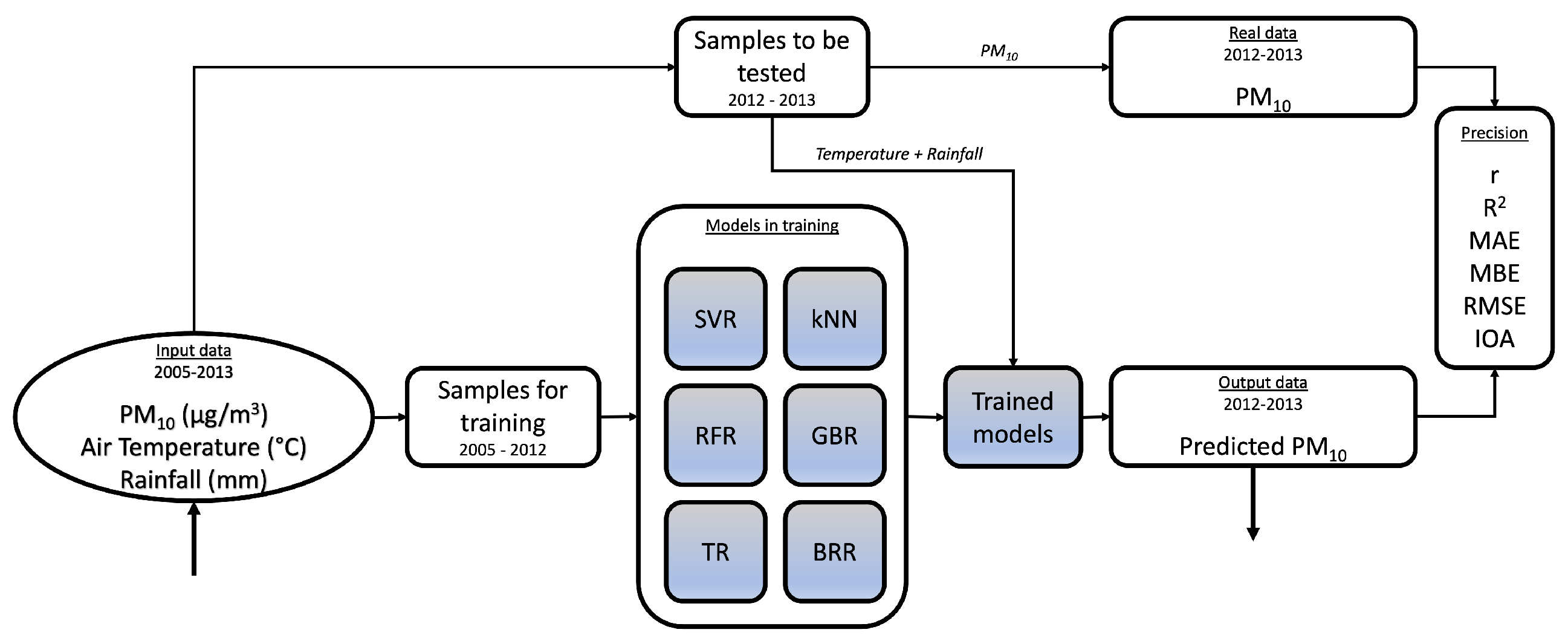
4.2. Machine Learning Process

To apply the six ML models, the dataset was fragmented into two groups, i.e., a learning set and an evaluation set using the scikit-learn library in Python. For the learning part, seven years (2005–2012) were selected, while for the evaluation part, one year (2012–2013) was used. Figure 2 shows a flowchart highlighting the methodology performed to apply and validate the models.

As described in Section 3.1, the success of each model depends on the chosen parameters. In the ML frame, it is crucial to find the proper mix between robustness and flexibility [36]. After extensive testing, the parameters that provided the best results were chosen, which are presented in

Table 2. Machine learning parameters for the models.

	Parameter 1	Parameter 2	Parameter 3	Parameter 4
SVR	RBF function	C ∼ 1000	γ ∼ 0.01	-
kNN	k = 3	Euclidean distance	-	-
RFR	tree number ∼ 100	max depth	square error	-
GBR	Loss function	true number ∼ 100	v ∼ 0.1	square error
TR	ξ ∼ 1.5	max iter ∼ 100	tolerance ∼ 1 × 10−6	-
BRR	a ∼ 1	max iter ∼ 200	tolerance ∼ 1 × 10−6	-

:

• For SVR, the kernel RBF was used with a large C (∼1000) and a small $\gamma$ (∼0.01);
• For kNN, k = 3 using $Euclideandistance$;
• For RFR, the parameters were chosen according to a trade-off between the time of process and accuracy. Thus, the bootstrap method was activated with the criterion squared error for high-quality data slicing. For the best accuracy, 100 trees (tree number) were specified in the forest with a max depth until all leaves were pure;
• For GBR, the same parameters as those of RFR were used, i.e., 100 trees and squared error function as the criterion. Furthermore, the squared error function was selected as a loss function with a learning rate of 0.1 to reduce the effect of the first tree in the decision tree;
• For TR, the Poisson–Gamma distribution was used. In the literature, numerous studies have already shown that $P{M}_{10}$ data in the Caribbean area do not follow a normal distribution [14,73];
• For BRR, parameters were chosen to stop the algorithm when the process converged to ∼$1\times {10}^{-6}$.

4.3. Machine Learning Forecasting

Figure 3 shows the results obtained for the six forecast models. Visually, the forecasts seem to give satisfactory results.

All the models followed the seasonal behavior of $P{M}_{10}$ linked to the African dust. By carrying out an analysis of ML curves, we nevertheless identified some mismatches between the empirical data and the models. For SVR and BRR, the predicted signal did not reach the maximum $P{M}_{10}$ concentrations, and the minimum values were negative. The maximum predicted $P{M}_{10}$ was around 60 μg/m³, while the measured $P{M}_{10}$ was 90 μg/m³. kNN exhibited the opposite behavior of SVR. The predicted signal exceeded the maximum $P{M}_{10}$ measured, while the minimum values were positive. For RFR, even if the predicted $P{M}_{10}$ signal tended toward zero when it was needed, the maximum was not high enough as for SVR (∼60 μg/m³). GBR exhibited the same behavior as RFR, but the maximum of predicted $P{M}_{10}$ was higher (∼70 μg/m³). As for TR, the predicted $P{M}_{10}$ had the same trends as the empirical signal but did not reach these upper and lower bounds.

4.4. Performance Analysis

To qualitatively estimate the robustness of the models, six performance indices were used. Overall, in

Table 3. Performance of machine learning models. Bold values indicate the best performance.

	SVR	kNN	RFR	GBR	TR	BRR
r	0.7641	0.6763	0.7524	0.7831	0.7443	0.7666
$R^2$	0.5839	0.4573	0.5661	0.6132	0.5540	0.5877
$MAE$	7.1298	8.4067	7.2015	6.8479	7.7303	7.4590
$MBE$	−2.8139	−0.4023	−0.2696	−1.1010	−1.2586	−0.5722
$RMSE$	11.2348	12.4251	10.9713	10.4400	11.3701	10.7435
$IOA$	0.7259	0.6768	0.7232	0.7368	0.7028	0.7133

, one can notice that GBR gave the best performance, as it exhibited the highest values of r-$R^2$-$IOA$ and the lowest values of $MAE$-$RMSE$. kNN was the model with the worst results. For all models, there were small negative values for $MBE$, indicating that the prediction tended to slightly underestimate $P{M}_{10}$ concentrations. According to Yang and Yang [64], BRR is a robust model to predict environmental data. $R^2$, $MAE$, and $RMSE$ performances obtained in Guadeloupe with GBR were better than those found in Ankara (Turkey) [44] with artificial neural networks (ANNs), which gave the best results to predict $P{M}_{10}$ time series ($R^2$ = 0.58, $MAE$ = 14.40, and $RMSE$ = 20.80). In London (United Kingdom) [43], the values of ANN (r = 0.80 and $IOA$ = 0.74), which also had the best performance, were also close to those we found.

It is important to underline that in the previous studies in Ankara and London, many input variables were used for ML models. In our study, only three variables were used. These results show the feature of $P{M}_{10}$ concentrations in the Caribbean basin. In this area, high $P{M}_{10}$ levels are mainly due to natural large-scale sources, i.e., the African dust [14,15]. Indeed, in the Caribbean islands, the background atmosphere is mainly composed of anthropogenic pollution and marine aerosols [74,75,76]. Anthropogenic pollution is low in Guadeloupe [49]. Without the dust haze that generates high $P{M}_{10}$ peaks, $P{M}_{10}$ behavior highlights a form of persistence between 20 and 25 μg/m³, i.e., the fluctuations are weak (see Figure 3) [77]. In megacities such as Ankara and London, anthropogenic pollution is high and mainly due to vehicle emissions. By performing a principal component analysis, Suleiman et al. [43] showed that vehicle emissions are the most important variable to predict $P{M}_{10}$ concentrations. This confirms the results of studies in Europe or China showing that motor vehicles are considered to be the main source of particles in the ABL due to heavy road traffic [78,79]. In other words, apart from the fact that $P{M}_{10}$ sources seem more heterogeneous in megacities, the impact of anthropogenic pollution on their concentrations is more significant than in the Caribbean area.

5. Conclusions

Due to the African dust recurrence in the Caribbean basin and its health impact, it is crucial to predict $P{M}_{10}$ concentrations. To carry out this study, six machine learning (ML) models were used: support vector regression (SVR), k-nearest neighbor regression (kNN), random forest regression (RFR), gradient boosting regression (GBR), Tweedie regression (TR) and Bayesian ridge regression (BRR). In addition to $P{M}_{10}$ data as the input parameters for the models, two climatic parameters that strongly impact African dust deposition in the ABL were used, i.e., air temperature and rainfall.

The results showed that GBR (r = 0.7831, $R^2$ = 0.6132, $MAE$ = 6.8479, $RMSE$ = 10.4400, and $IOA$ = 0.7368) was the model with the best performance, while kNN (r = 0.6763, $R^2$ = 0.4573, $MAE$ = 8.4067, $RMSE$ = 12.4251, and $IOA$ = 0.6768) had the worst performance. The authors assume that the fact that GBR has a greater ability to predict extreme events may explain this result. Indeed, dust outbreaks are random events that continuously vary in duration and intensity. Due to the low heterogeneity of $P{M}_{10}$ sources in the Caribbean islands, significant results were obtained with only three input parameters, whereas in Europe or China, many parameters are required. All these results clearly highlight the feature of $P{M}_{10}$ concentrations behavior in the Caribbean.

In ML studies, it is important to use several models to perform forecasting. Indeed, in addition to model specificities, the inherent properties of the time series will also influence the efficiency of the prediction. Consequently, a $P{M}_{10}$ ML model that works perfectly for one location may perform poorly for another place.

Even if the GBR model yielded significant results, its performance can be improved. In future work, the first step will be to add other variables that were not available for this study, i.e., particles lower or equal to 2.5 μm in diameter ($P{M}_{2.5}$) and other meteorological parameters (solar radiation, wind speed, relative humidity, and pressure).

References

1. Saco, P.; McDonough, K.; Rodriguez, J.; Rivera-Zayas, J.; Sandi, S. The role of soils in the regulation of hazards and extreme events. Philos. Trans. R. Soc. B 2021, 376, 20200178. [Google Scholar] [CrossRef] [PubMed]
2. Euphrasie-Clotilde, L.; Plocoste, T.; Brute, F. Particle Size Analysis of African Dust Haze over the Last 20 Years: A Focus on the Extreme Event of June 2020. Atmosphere 2021, 12, 502. [Google Scholar] [CrossRef]
3. Plocoste, T. Multiscale analysis of the dynamic relationship between particulate matter (PM10) and meteorological parameters using CEEMDAN: A focus on “Godzilla” African dust event. Atmos. Pollut. Res. 2022, 13, 101252. [Google Scholar] [CrossRef]
4. Urrutia-Pereira, M.; Rizzo, L.; Staffeld, P.; Chong-Neto, H.; Viegi, G.; Solé, D. Dust from the Sahara to the American Continent: Health impacts: Dust from Sahara. Allergol. Immunopathol. 2021, 49, 187–194. [Google Scholar] [CrossRef] [PubMed]
5. Gyan, K.; Henry, W.; Lacaille, S.; Laloo, A.; Lamsee-Ebanks, C.; McKay, S.; Antoine, R.; Monteil, M. African dust clouds are associated with increased paediatric asthma accident and emergency admissions on the Caribbean island of Trinidad. Int. J. Biometeorol. 2005, 49, 371–376. [Google Scholar] [CrossRef]
6. Monteil, M. Saharan dust clouds and human health in the English-speaking Caribbean: What we know and don’t know. Environ. Geochem. Health 2008, 30, 339–343. [Google Scholar] [CrossRef]
7. Cadelis, G.; Tourres, R.; Molinié, J. Short-term effects of the particulate pollutants contained in Saharan dust on the visits of children to the emergency department due to asthmatic conditions in Guadeloupe (French Archipelago of the Caribbean). PLoS ONE 2014, 9, e91136. [Google Scholar] [CrossRef] [Green Version]
8. Akpinar-Elci, M.; Martin, F.; Behr, J.; Diaz, R. Saharan dust, climate variability, and asthma in Grenada, the Caribbean. Int. J. Biometeorol. 2015, 59, 1667–1671. [Google Scholar] [CrossRef]
9. Viel, J.; Michineau, L.; Garbin, C.; Monfort, C.; Kadhel, P.; Multigner, L.; Rouget, F. Impact of Saharan Dust on Severe Small for Gestational Births in the Caribbean. Am. J. Trop. Med. Hyg. 2020, 102, 1463–1465. [Google Scholar] [CrossRef]
10. Carlson, T.; Prospero, J. The large-scale movement of Saharan air outbreaks over the northern equatorial Atlantic. J. Appl. Meteorol. Climatol. 1972, 11, 283–297. [Google Scholar] [CrossRef]
11. Prospero, J.; Carlson, T. Vertical and areal distribution of Saharan dust over the western equatorial North Atlantic Ocean. J. Geophys. Res. 1972, 77, 5255–5265. [Google Scholar] [CrossRef] [Green Version]
12. Prospero, J.; Delany, A.; Delany, A.; Carlson, T. The Discovery of African Dust Transport to the Western Hemisphere and the Saharan Air Layer: A History. Bull. Am. Meteorol. Soc. 2021, 102, E1239–E1260. [Google Scholar] [CrossRef]
13. Prospero, J.; Collard, F.; Molinié, J.; Jeannot, A. Characterizing the annual cycle of African dust transport to the Caribbean Basin and South America and its impact on the environment and air quality. Glob. Biogeochem. Cycles 2014, 28, 757–773. [Google Scholar] [CrossRef]
14. Plocoste, T.; Calif, R.; Euphrasie-Clotilde, L.; Brute, F. The statistical behavior of PM10 events over guadeloupean archipelago: Stationarity, modelling and extreme events. Atmos. Res. 2020, 241, 104956. [Google Scholar] [CrossRef]
15. Plocoste, T.; Euphrasie-Clotilde, L.; Calif, R.; Brute, F. Quantifying spatio-temporal dynamics of African dust detection threshold for PM10 concentrations in the Caribbean area using multiscale decomposition. Front. Environ. Sci. 2022, 10, 907440. [Google Scholar] [CrossRef]
16. Schepanski, K. Transport of mineral dust and its impact on climate. Geosciences 2018, 8, 151. [Google Scholar] [CrossRef] [Green Version]
17. Plocoste, T.; Calif, R. Is there a causal relationship between Particulate Matter (PM10) and air Temperature data? An analysis based on the Liang-Kleeman information transfer theory. Atmos. Pollut. Res. 2021, 12, 101177. [Google Scholar] [CrossRef]
18. Plocoste, T. Detecting the Causal Nexus between Particulate Matter (PM10) and Rainfall in the Caribbean Area. Atmosphere 2022, 13, 175. [Google Scholar] [CrossRef]
19. Elminir, H.K. Relative influence of air pollutants and weather conditions on solar radiation—Part 1: Relationship of air pollutants with weather conditions. Meteorol. Atmos. Phys. 2007, 96, 245–256. [Google Scholar] [CrossRef]
20. Plocoste, T.; Calif, R.; Euphrasie-Clotilde, L.; Brute, F. Investigation of local correlations between particulate matter (PM10) and air temperature in the Caribbean basin using Ensemble Empirical Mode Decomposition. Atmos. Pollut. Res. 2020, 11, 1692–1704. [Google Scholar] [CrossRef]
21. Zhu, L.; Liu, J.; Cong, L.; Ma, W.; Ma, W.; Zhang, Z. Spatiotemporal characteristics of particulate matter and dry deposition flux in the Cuihu wetland of Beijing. PLoS ONE 2016, 11, e0158616. [Google Scholar] [CrossRef] [PubMed] [Green Version]
22. Wu, Y.; Liu, J.; Zhai, J.; Cong, L.; Wang, Y.; Ma, W.; Zhang, Z.; Li, C. Comparison of dry and wet deposition of particulate matter in near-surface waters during summer. PLoS ONE 2018, 13, e0199241. [Google Scholar] [CrossRef] [PubMed]
23. Fan, J.; Wang, Y.; Rosenfeld, D.; Liu, X. Review of aerosol–cloud interactions: Mechanisms, significance, and challenges. J. Atmos. Sci. 2016, 73, 4221–4252. [Google Scholar] [CrossRef]
24. Plocoste, T.; Carmona-Cabezas, R.; Gutiérrez de Ravé, E.; Jimnez-Hornero, F. Wet scavenging process of particulate matter (PM10): A multivariate complex network approach. Atmos. Pollut. Res. 2021, 12, 101095. [Google Scholar] [CrossRef]
25. Sugihara, G.; May, R.; Ye, H.; Hsieh, C.; Deyle, E.; Fogarty, M.; Munch, S. Detecting causality in complex ecosystems. Science 2012, 338, 496–500. [Google Scholar] [CrossRef] [PubMed]
26. Konovalov, I.; Beekmann, M.; Meleux, F.; Dutot, A.; Foret, G. Combining deterministic and statistical approaches for PM10 forecasting in Europe. Atmos. Environ. 2009, 43, 6425–6434. [Google Scholar] [CrossRef]
27. Lee, H.; Liu, Y.; Coull, B.; Schwartz, J.; Koutrakis, P. A novel calibration approach of MODIS AOD data to predict PM2.5 concentrations. Atmos. Chem. Phys. 2011, 11, 7991–8002. [Google Scholar] [CrossRef] [Green Version]
28. Chen, Y.; Shi, R.; Shu, S.; Gao, W. Ensemble and enhanced PM10 concentration forecast model based on stepwise regression and wavelet analysis. Atmos. Environ. 2013, 74, 346–359. [Google Scholar] [CrossRef]
29. Djalalova, I.; Delle Monache, L.; Wilczak, J. PM2.5 analog forecast and Kalman filter post-processing for the Community Multiscale Air Quality (CMAQ) model. Atmos. Environ. 2015, 108, 76–87. [Google Scholar] [CrossRef]
30. Kloog, I.; Chudnovsky, A.A.; Just, A.C.; Nordio, F.; Koutrakis, P.; Coull, B.A.; Lyapustin, A.; Wang, Y.; Schwartz, J. A new hybrid spatio-temporal model for estimating daily multi-year PM2.5 concentrations across northeastern USA using high resolution aerosol optical depth data. Atmos. Environ. 2014, 95, 581–590. [Google Scholar] [CrossRef]
31. Hu, X.; Belle, J.H.; Meng, X.; Wildani, A.; Waller, L.A.; Strickland, M.J.; Liu, Y. Estimating PM2.5 concentrations in the conterminous United States using the random forest approach. Environ. Sci. Technol. 2017, 51, 6936–6944. [Google Scholar] [CrossRef] [PubMed]
32. Chen, G.; Wang, Y.; Li, S.; Cao, W.; Ren, H.; Knibbs, L.D.; Abramson, M.J.; Guo, Y. Spatiotemporal patterns of PM10 concentrations over China during 2005–2016: A satellite-based estimation using the random forests approach. Environ. Pollut. 2018, 242, 605–613. [Google Scholar] [CrossRef] [PubMed]
33. Choubin, B.; Moradi, E.; Golshan, M.; Adamowski, J.; Sajedi-Hosseini, F.; Mosavi, A. An ensemble prediction of flood susceptibility using multivariate discriminant analysis, classification and regression trees, and support vector machines. Sci. Total Environ. 2019, 651, 2087–2096. [Google Scholar] [CrossRef]
34. Mahesh, B. Machine learning algorithms-a review. Int. J. Sci. Res. 2020, 9, 381–386. [Google Scholar]
35. Choubin, B.; Abdolshahnejad, M.; Moradi, E.; Querol, X.; Mosavi, A.; Shamshirband, S.; Ghamisi, P. Spatial hazard assessment of the PM10 using machine learning models in Barcelona, Spain. Sci. Total Environ. 2020, 701, 134474. [Google Scholar] [CrossRef] [PubMed]
36. Zickus, M.; Greig, A.; Niranjan, M. Comparison of four machine learning methods for predicting PM10 concentrations in Helsinki, Finland. Water Air Soil Pollut. Focus 2002, 2, 717–729. [Google Scholar] [CrossRef]
37. Brodley, C.E. Addressing the selective superiority problem: Automatic algorithm/model class selection. In Proceedings of the Tenth International Conference on Machine Learning, Amherst, MA, USA, 27–29 June 1993; pp. 17–24. [Google Scholar]
38. Raimondo, G.; Montuori, A.; Moniaci, W.; Pasero, E.; Almkvist, E. A machine learning tool to forecast PM10 level. In Proceedings of the AMS 87th Annual Meeting, San Antonio, TX, USA, 14–18 January 2007; pp. 13–18. [Google Scholar]
39. Voukantsis, D.; Karatzas, K.; Kukkonen, J.; Räsänen, T.; Karppinen, A.; Kolehmainen, M. Intercomparison of air quality data using principal component analysis, and forecasting of PM10 and PM2.5 concentrations using artificial neural networks, in Thessaloniki and Helsinki. Sci. Total Environ. 2011, 409, 1266–1276. [Google Scholar] [CrossRef]
40. de Gennaro, G.; Trizio, L.; Di Gilio, A.; Pey, J.; Pérez, N.; Cusack, M.; Alastuey, A.; Querol, X. Neural network model for the prediction of PM10 daily concentrations in two sites in the Western Mediterranean. Sci. Total Environ. 2013, 463, 875–883. [Google Scholar] [CrossRef]
41. Debry, E.; Mallet, V. Ensemble forecasting with machine learning algorithms for ozone, nitrogen dioxide and PM10 on the Prev’Air platform. Atmos. Environ. 2014, 91, 71–84. [Google Scholar] [CrossRef]
42. Taspinar, F. Improving artificial neural network model predictions of daily average PM10 concentrations by applying principle component analysis and implementing seasonal models. J. Air Waste Manag. Assoc. 2015, 65, 800–809. [Google Scholar] [CrossRef]
43. Suleiman, A.; Tight, M.; Quinn, A. Applying machine learning methods in managing urban concentrations of traffic-related particulate matter (PM10 and PM2.5). Atmos. Pollut. Res. 2019, 10, 134–144. [Google Scholar] [CrossRef]
44. Bozdağ, A.; Dokuz, Y.; Gökçek, Ö.B. Spatial prediction of PM10 concentration using machine learning algorithms in Ankara, Turkey. Environ. Pollut. 2020, 263, 114635. [Google Scholar] [CrossRef] [PubMed]
45. Kim, B.Y.; Lim, Y.K.; Cha, J.W. Short-term prediction of particulate matter (PM10 and PM2.5) in Seoul, South Korea using tree-based machine learning algorithms. Atmos. Pollut. Res. 2022, 13, 101547. [Google Scholar] [CrossRef]
46. Kujawska, J.; Kulisz, M.; Oleszczuk, P.; Cel, W. Machine Learning Methods to Forecast the Concentration of PM10 in Lublin, Poland. Energies 2022, 15, 6428. [Google Scholar] [CrossRef]
47. Plocoste, T.; Calif, R.; Jacoby-Koaly, S. Multi-scale time dependent correlation between synchronous measurements of ground-level ozone and meteorological parameters in the Caribbean Basin. Atmos. Environ. 2019, 211, 234–246. [Google Scholar] [CrossRef]
48. Plocoste, T.; Jacoby-Koaly, S.; Molinié, J.; Petit, R. Evidence of the effect of an urban heat island on air quality near a landfill. Urban Clim. 2014, 10, 745–757. [Google Scholar] [CrossRef]
49. Plocoste, T.; Dorville, J.; Monjoly, S.; Jacoby-Koaly, S.; André, M. Assessment of Nitrogen Oxides and Ground-Level Ozone behavior in a dense air quality station network: Case study in the Lesser Antilles Arc. J. Air Waste Manag. Assoc. 2018, 68, 1278–1300. [Google Scholar] [CrossRef] [Green Version]
50. Plocoste, T.; Calif, R.; Jacoby-Koaly, S. Temporal multiscaling characteristics of particulate matter PM10 and ground-level ozone O3 concentrations in Caribbean region. Atmos. Environ. 2017, 169, 22–35. [Google Scholar] [CrossRef]
51. Plocoste, T.; Pavón-Domínguez, P. Multifractal detrended cross-correlation analysis of wind speed and solar radiation. Chaos Interdiscip. J. Nonlinear Sci. 2020, 30, 113109. [Google Scholar] [CrossRef]
52. Gani, W.; Taleb, H.; Limam, M. Support vector regression based residual control charts. J. Appl. Stat. 2010, 37, 309–324. [Google Scholar] [CrossRef]
53. Singh, A.; Kotiyal, V.; Sharma, S.; Nagar, J.; Lee, C.C. A machine learning approach to predict the average localization error with applications to wireless sensor networks. IEEE Access 2020, 8, 208253–208263. [Google Scholar] [CrossRef]
54. Bodaghi, A.; Ansari, H.R.; Gholami, M. Optimized support vector regression for drillingrate of penetration estimation. Open Geosci. 2015, 7, 870–879. [Google Scholar] [CrossRef] [Green Version]
55. Drucker, H.; Burges, C.J.; Kaufman, L.; Smola, A.; Vapnik, V. Support vector regression machines. Adv. Neural Inf. Process. Syst. 1996, 9. [Google Scholar]
56. Guo, Y.; Li, X.; Bai, G.; Ma, J. Time series prediction method based on LS-SVR with modified gaussian RBF. In Proceedings of the International Conference on Neural Information Processing, Doha, Qatar, 12–15 November 2012; Springer: Berlin/Heidelberg, Germany, 2012; pp. 9–17. [Google Scholar]
57. Zhang, S.; Li, X.; Zong, M.; Zhu, X.; Cheng, D. Learning k for knn classification. ACM Trans. Intell. Syst. Technol. (TIST) 2017, 8, 1–19. [Google Scholar] [CrossRef] [Green Version]
58. Ban, T.; Zhang, R.; Pang, S.; Sarrafzadeh, A.; Inoue, D. Referential knn regression for financial time series forecasting. In Proceedings of the International Conference on Neural Information Processing, Daegu, Republic of Korea, 3–7 November 2013; Springer: Berlin/Heidelberg, Germany, 2013; pp. 601–608. [Google Scholar]
59. Breiman, L. Random forests. Mach. Learn. 2001, 45, 5–32. [Google Scholar] [CrossRef] [Green Version]
60. Segal, M.R. Machine Learning Benchmarks and Random Forest Regression; Technical Report; University of California: California, CA, USA, 2004. [Google Scholar]
61. Natekin, A.; Knoll, A. Gradient boosting machines, a tutorial. Front. Neurorobotics 2013, 7, 21. [Google Scholar] [CrossRef] [Green Version]
62. Keprate, A.; Ratnayake, R.C. Using gradient boosting regressor to predict stress intensity factor of a crack propagating in small bore piping. In Proceedings of the 2017 IEEE International Conference on Industrial Engineering and Engineering Management (IEEM), Singapore, 10–13 December 2017; IEEE: Piscataway, NJ, USA, 2017; pp. 1331–1336. [Google Scholar]
63. Smyth, G.K. Regression analysis of quantity data with exact zeros. In Proceedings of the Second Australia–Japan Workshop on Stochastic Models in Engineering, Technology and Management, Gold Coast, Australia, 17–19 July 1996; Citeseer: Princeton, NJ, USA, 1996; pp. 572–580. [Google Scholar]
64. Yang, Y.; Yang, Y. Hybrid prediction method for wind speed combining ensemble empirical mode decomposition and Bayesian ridge regression. IEEE Access 2020, 8, 71206–71218. [Google Scholar] [CrossRef]
65. Ul-Saufie, A.Z.; Yahya, A.S.; Ramli, N.A.; Hamid, H.A. Comparison between multiple linear regression and feed forward back propagation neural network models for predicting PM10 concentration level based on gaseous and meteorological parameters. Int. J. Appl. Sci. Technol. 2011, 1, 42–49. [Google Scholar]
66. Willmott, C.J.; Robeson, S.M.; Matsuura, K. A refined index of model performance. Int. J. Climatol. 2012, 32, 2088–2094. [Google Scholar] [CrossRef]
67. Fu, M.; Wang, W.; Le, Z.; Khorram, M.S. Prediction of particular matter concentrations by developed feed-forward neural network with rolling mechanism and gray model. Neural Comput. Appl. 2015, 26, 1789–1797. [Google Scholar] [CrossRef]
68. Papoulis, A.; Pillai, S.U. Probability, Random Variables, and Stochastic Processes; Tata McGraw-Hill Education: New York, NY, USA, 2002. [Google Scholar]
69. Windsor, H.; Toumi, R. Scaling and persistence of UK pollution. Atmos. Environ. 2001, 35, 4545–4556. [Google Scholar] [CrossRef]
70. Barkstrom, B.R.; Smith, G.L. The earth radiation budget experiment: Science and implementation. Rev. Geophys. 1986, 24, 379–390. [Google Scholar] [CrossRef]
71. Martinez, C.; Goddard, L.; Kushnir, Y.; Ting, M. Seasonal climatology and dynamical mechanisms of rainfall in the Caribbean. Clim. Dyn. 2019, 53, 825–846. [Google Scholar] [CrossRef]
72. Martinez, C.; Kushnir, Y.; Goddard, L.; Ting, M. Interannual variability of the early and late-rainy seasons in the Caribbean. Clim. Dyn. 2020, 55, 1563–1583. [Google Scholar] [CrossRef]
73. Alexis, E.; Plocoste, T.; Nuiro, S.P. Analysis of Particulate Matter (PM10) Behavior in the Caribbean Area Using a Coupled SARIMA-GARCH Model. Atmosphere 2022, 13, 862. [Google Scholar] [CrossRef]
74. Clergue, C.; Dellinger, M.; Buss, H.; Gaillardet, J.; Benedetti, M.; Dessert, C. Influence of atmospheric deposits and secondary minerals on Li isotopes budget in a highly weathered catchment, Guadeloupe (Lesser Antilles). Chem. Geol. 2015, 414, 28–41. [Google Scholar] [CrossRef] [Green Version]
75. Rastelli, E.; Corinaldesi, C.; Dell’Anno, A.; Martire, M.; Greco, S.; Facchini, M.; Rinaldi, M.; O’Dowd, C.; Ceburnis, D.; Danovaro, R. Transfer of labile organic matter and microbes from the ocean surface to the marine aerosol: An experimental approach. Sci. Rep. 2017, 7, 11475. [Google Scholar] [CrossRef]
76. Plocoste, T.; Carmona-Cabezas, R.; Jiménez-Hornero, F.; Gutiérrez de Ravé, E. Background PM10 atmosphere: In the seek of a multifractal characterization using complex networks. J. Aerosol Sci. 2021, 155, 105777. [Google Scholar] [CrossRef]
77. Plocoste, T.; Carmona-Cabezas, R.; Jiménez-Hornero, F.J.; Gutiérrez de Ravé, E.; Calif, R. Multifractal characterisation of particulate matter (PM10) time series in the Caribbean basin using visibility graphs. Atmos. Pollut. Res. 2021, 12, 100–110. [Google Scholar] [CrossRef]
78. Künzli, N.; Kaiser, R.; Medina, S.; Studnicka, M.; Chanel, O.; Filliger, P.; Herry, M.; Horak, F.; Puybonnieux-Texier, V.; Quénel, P.; et al. Public-health impact of outdoor and traffic-related air pollution: A European assessment. Lancet 2000, 356, 795–801. [Google Scholar] [CrossRef]
79. He, H.; Pan, W.; Lu, W.; Xue, Y.; Peng, G. Multifractal property and long-range cross-correlation behavior of particulate matters at urban traffic intersection in Shanghai. Stoch. Environ. Res. Risk Assess. 2016, 30, 1515–1525. [Google Scholar] [CrossRef]
Figure 1. Synchronous measurements of (a) P M 10 concentrations, (b) air temperature (T), and (c) rainfall ( R R ) from 2005 to 2012.
Atmosphere 14 00134 g001
Figure 2. A flowchart describing the methodology performed to apply and validate the machine learning models.
Atmosphere 14 00134 g002
Figure 3. Daily P M 10 time series predicted by the machine learning models.
Atmosphere 14 00134 g003