Article

Statistical Characteristics of Blocking High in the Ural Mountains during Winters and Relationship with Changes in Sea Surface Temperature and Sea Ice

1
School of Marine Sciences, Nanjing University of Information Science and Technology, Nanjing 210044, China
2
Department of Geography and Resource Management, Chinese University of Hong Kong, Hong Kong 999777, China
*
Author to whom correspondence should be addressed.
Atmosphere 2023, 14(1), 129; https://doi.org/10.3390/atmos14010129
Submission received: 16 December 2022 / Revised: 3 January 2023 / Accepted: 3 January 2023 / Published: 6 January 2023
(This article belongs to the Special Issue Atmospheric Blocking and Weather Extremes)

Abstract

:
A blocking high in the Ural Mountains, which is recognized as the third major blocking high area in the northern hemisphere, describes a deep warm high-pressure system superimposed on the westerly belt. Based on the ERA-5 daily reanalysis data (the fifth-generation European Centre for Medium-Range Weather Forecasts atmospheric reanalysis global climate dataset) and using the Tibaldi and Molteni (TM) method, we selected 43 blocking high events in the Ural Mountains during the extended winters of 1979–2020 and analyzed their atmospheric circulation characteristics and influencing factors. Our findings revealed a downward trend in the frequency of occurrence of blocking highs in the Ural Mountains in winter, most of them were short-lived; furthermore, the frequency and duration of these occurrences generally followed a 3–4 years oscillating cycle. The synthetic results of the geopotential height (HGT) anomaly field and the surface air temperature (SAT) anomaly field of these 43 extended wintertime blocking high events in the Ural Mountains region showed that during the development of a blocking high, the central intensity of the positive anomalies in the Ural Mountains region first increased and then weakened, while the central intensity and meridional span of the negative anomalies in the Eurasian mid-latitudes of the SAT anomaly field increased continuously. In addition, abnormally high sea surface temperature (SST) in the North Atlantic sea area and abnormal reduction of sea ice (SI) in the Barents-Kara Sea and the Chukchi Sea in autumn had a significant impact on the wintertime formation of Ural Mountains blocking highs. In contrast, in autumn, the abnormal reduction of SI in the Barents-Kara and Chukchi Seas might also have led to the westward positioning of Ural Mountains blocking highs.

1. Introduction

A blocking high is formed when a long-wave ridge system develops and evolves in the westerly belt. As the high-pressure ridge extends northward, cold air severs the connection between the south side of the ridge and the warm air in the south, and a closed circulation appears on the north side of the ridge, thus forming the center of a warm high-pressure system. In Asia, blocking highs are well known in the Lake Baikal region, the Ural Mountains region, and the Sea of Okhotsk region. While blocking highs in Asia are generally common in autumn and winter, in the Sea of Okhotsk, in particular, they mainly occur during the summer [1]. However, in the context of global warming, the frequency of blocking highs is decreasing [2].
The Ural Mountains, located in Russia, have a northeast-southwest tilt. This mountain range has long been considered the dividing line between Europe and Asia. This region belongs to the continental climate category, which is characterized by obvious temperature polarization. In addition, it has long been of interest to meteorologists because of its special geographical location [3]. In meteorological studies, the Ural Mountains area typically refers to the area of 50° E–80° E. Closed warm high-pressure systems, known as Ural Mountains blocking highs (also referred to as Siberian blocking highs), often occur in this region in winter. The appearance of this phenomenon is usually accompanied by an intensification of the cold advection in the downstream area, which directly results in an abnormally low-temperature phenomenon in East Asia, especially China [4,5,6]. For example, in January 2008, many provinces (including Jiangsu, Hunan, and Fujian) in southern China experienced severe low-temperature rain, snow, and freezing disasters, with extremely serious impacts on the life and production of people living in the region, which were attributed to the continuous abnormal activities of a Ural Mountains blocking high [4], and another strong Ural Mountains blocking high was connected to a strong cold front that similarly hit China in January 2016 [6]. This process caused East China to experience extremely low temperatures of about −10 °C; at the same time, the lowest temperature in South China, which reached 0 °C, greatly affected industrial and agricultural production and residents’ lives [5].
Many factors influence blocking highs, including stratospheric explosive warming [7], the sea surface temperature (SST) anomaly [8], the East Asian monsoon anomaly [9], and the sea ice (SI) anomaly [10], all these factors which have a significant impact on the formation, development, maintenance, and decline of a blocking high. In recent years, many meteorological researchers have studied the factors affecting the Ural Mountains blocking highs in winter [11,12,13,14]. For example, Cheung et al. [11] pointed out that if both AO (Arctic Oscillation) and ENSO (El Niño–Southern Oscillation) reached the positive (negative) phase, the Ural-Siberia blocking high tended to be less (more); Ma et al. [13] showed that the SIC perturbations in the Greenland Sea (GS), Barents Sea (BS) and Okhotsk Sea (OKS) had significances for the strong and persistent prediction of UB formation. Furthermore, Lu et al. [14] found that the long-lived blocking high frequency of the Ural Mountains tended to weaken during the winter of 1979–2018, and the poleward transport of constant momentum flux in the northwest-southeast region of the Ural Mountains blocking high key areas on the 500–300 hPa was a key factor to maintain the blocking high for a long time.
Under the background of global warming, the anomaly of SST and SI play an increasingly important role in the change of atmospheric circulation (especially the persistent anomalies of blocking high) [15,16,17,18]. Correspondingly, SI ablation and its climate effects on mid-latitude weather and climate have drawn increasing interest in the field of climate change research [19,20]. Additionally, the frequency of cold wave events in the past 50 years has shown an overall downward trend, but a fluctuating upward trend since the 1990s, and cold wave events mainly occurred in November, December, and March [21]. What is more, some studies have pointed out that the frequent occurrence of cold waves in East Asia was related to the changes in the characteristics and evolution mechanism of blocking high in the middle and upper latitudes against the context of global warming [22]. On that basis, we try to explore the changing characteristics of the blocking high in the Ural Mountains in extended winter (November–March) from a long time scale, and identify the key regions of SST and SI that affected the blocking high. The study findings thus provide a scientific reference for better understanding the formation mechanism of a blocking high in the Ural Mountains, along with medium and long-term weather forecasting and even short-term climate prediction.

2. Materials and Methods

2.1. Materials

This paper uses the fifth-generation ECMWF (European Centre for Medium-Range Weather Forecasts) atmospheric reanalysis global climate dataset (ERA-5) (https://cds.climate.copernicus.eu/#!/home) (accessed on 3 April 2022). The ERA-5 data provide hourly estimates of atmospheric, terrestrial, and oceanic climate variables, with Earth data accurate to a 30 km grid, including 137 layers of atmospheric data. The dataset is on a standard global longitude/latitude grid with 0.25° latitude and longitude intervals. A total of 42 extended winters from 1979 to 2021 were counted in this paper (the extended winter calculation standard, in which November–December 1979 and January–March 1980 were collectively referred to as the winter of 1979). The meteorological variables on the multiple levels used in this study are geopotential height (HGT), wind speed (U, V), and air temperature (T). Furthermore, surface turbulent heat flux (STHF, the sum of surface sensible and latent heat flux), and surface air temperature (SAT) of 2 m are also used in the study.
In addition, the SST and SI data used in this paper are Hadley Centre Sea Ice (SI) and SST data set (HadISST) provided by the Hadley Centre of the National Met Office in the United Kingdom, Exeter (https://hadleyserver.metoffice.gov.uk/hadisst/data/download.html) (accessed on 5 May 2022), which replaces the global sea ice and sea surface temperature data set (GISST), and is a unique combination of the global monthly complete SST and SI concentration on a 1-degree latitude and longitude grid from 1870 to the present. The data set consists of three parts: (1) field observation data of ships and buoys; (2) satellite data; and (3) ICOADS (International Comprehensive Ocean-Atmosphere Data Set) data [23]. The dataset is mainly downscaled through an interpolation process, and then the quality-improved grid observations are superimposed on the original data to supplement local details, thus achieving global coverage of the data [24]. The seasonal average calculation standards for SST and SI data are spring (March–May), summer (June–August), autumn (September–November), and winter (December–February).

2.2. Methods

2.2.1. Tibaldi and Molteni (TM) Method

The method used in this paper to calculate the blocking high is the TM method, which is mostly used by meteorologists [9,18,25,26]. The main advantages of the TM method are: simple and easy to operate; better identification of strong and stable obstruction; intuitive and clear. Lejnäs and Økland [27] defined the blocking high index as the difference between 500 hPa geopotential height between 40° N and 60° N. Subsequently, in order to ensure that there is an average westerly airflow with a wind speed of not less than 8 m/s in the direction of the blocking highs to polar, Tibaldi and Molteni [28] improved and perfected this method, which is now the widely used TM method. The specific steps of the TM method are as follows:
The HGT gradient was divided into the south 500 hPa HGT gradient and the north 500 hPa HGT gradient, which were, respectively, represented by GHGS (Southern Gradients of Geopotential Height) and GHGN (Northern Gradients of Geopotential Height). Then, calculate each longitude, respectively,
GHGS = Z 0 Z S 0 S
GHGN = Z N Z 0 N 0  
In the above Formulas (1) and (2), Z represents the 500 hPa HGT, N = 80 °   N + δ ,   0 = 60 °   N + δ , S = 40 °   N + δ ,   δ = 4 ° , 0 ° , 4 ° .
For any δ value of a certain longitude at a certain time, if the following two conditions can be satisfied:
(1)
GHGS > 0
(2)
GHGN < −10 m/latitude distances
Then, it can be judged that there is a blocking high at the longitude, and at this time, the judgment is an instantaneous blocking high, and GHGS is the blocking high index at this longitude [27].
In addition, when more than two δ values can satisfy the above two conditions, the one with the largest GHGS value is taken as the resistance height index, which can be used to judge the strength of the blocking high. For the blocking high in a certain area, it can be defined as if there are at least 15 consecutive longitudes that satisfy the conditions (1) and (2), it is judged that there is a blocking high in this area. When the duration of blocking high in this region reaches or exceeds 4 days, it is said that a “blocking high event” occurs in this region. The minimum duration can be adjusted according to the situation of blocking highs in this region. In this paper, the minimum duration of a blocking high event is defined as 5 days.

2.2.2. Morlet Wavelet Analysis Method

Wavelet analysis is an analysis method of signal time and frequency localization, which can expand a one-dimensional signal in both time and frequency directions, so as to clearly understand the frequency characteristics of time series in different time domains [29]. After years of development and application, wavelet transform has become a relatively mature mathematical analysis tool in the fields of atmospheric science, hydrology, and computer science [30,31]. The wavelet in the complex form has more advantages than the wavelet in the real form in application. The most commonly used wavelet function in the complex form is the Morlet wavelet. The real and imaginary parts of the Morlet wavelet can be treated as two wavelet functions, respectively. The real part is used to identify the structure of the signal at different spatiotemporal scales and the location of its abrupt points, while the imaginary part is an antisymmetric wavelet function.
The Morlet wavelet function has the following form:
Ψ t = C e t 2 / 2 / c o s 5 t
In the formula: Ψ t represents the mother wavelet, C is a constant, and t is time.
This paper uses the wavelet toolkit that comes with MATLAB software (MathWorks, Natick, Massachusetts, the United States) to carry out wavelet transform [32]. Before the analysis, in order to eliminate or reduce the boundary effect near the start point and end point of the sequence, the data were extended at both ends of the data to be consistent with the length of the original sequence. When the wavelet transform is completed, the wavelet transform coefficients extended at both ends are removed, and only the wavelet analysis coefficients corresponding to the original sequence are retained.

2.2.3. Synthetic Analysis

When studying climate change, we usually focus on the characteristics of certain specific time periods. The general approach is to combine samples with the same characteristics and analyze the similarities and differences. Common usage: (1) In the interannual change analysis, to synthesize high-value year data and low-value year data; (2) in the analysis of decadal change, synthesize data of different decadal periods; (3) synthesize some kind of the same event.
Synthetic analysis generally uses t test to construct statistic t:
t = x ¯ μ 0 S n  
where x ¯     and μ 0 are, respectively, sample mean and the population mean, S represents mean square error, and the sample size is n. Assuming that μ 0   does not change, then the statistic t follows the t-distribution of n − 1 degrees of freedom. If t t , then reject the null hypothesis, or accept the null hypothesis.
In this paper, is 0.05, which is a confident interval of 95%.

3. Results

3.1. Statistical Characteristics of Blocking Highs in Ural Mountains in Extended Winter

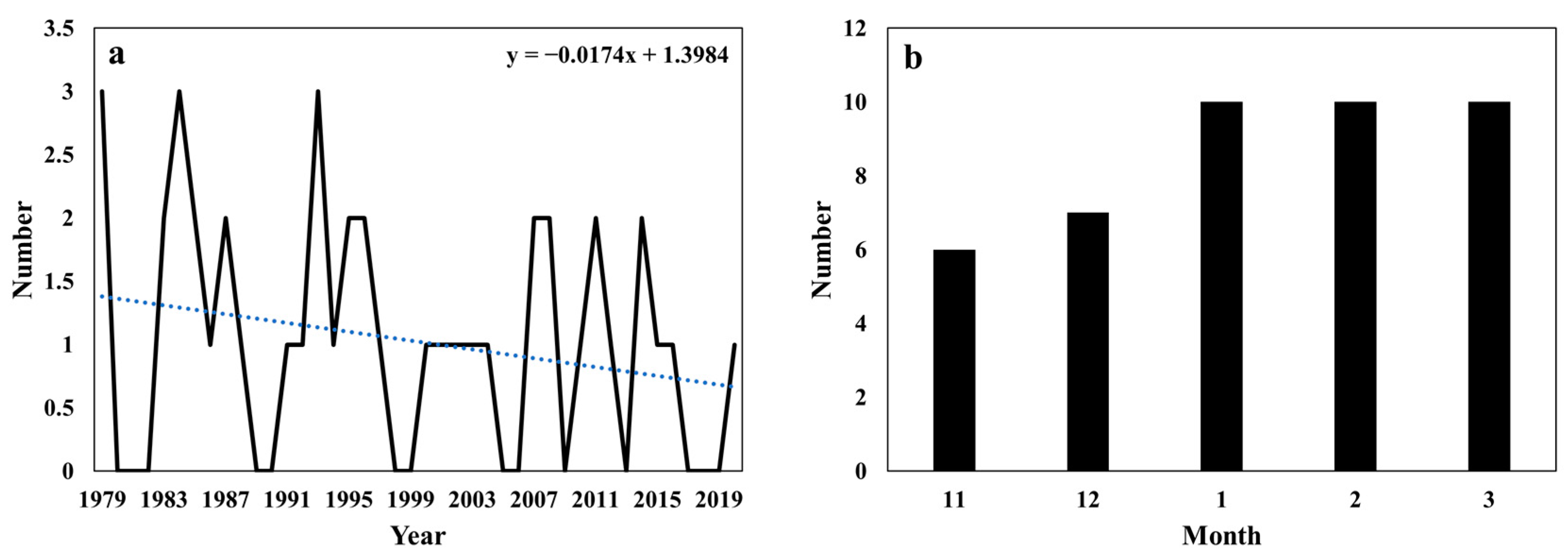
3.1.1. Change Characteristics of Frequency

This article takes the Ural Mountains region for (40°~80° E, 40°~70° N). According to the TM method, ERA5 data from 1 November 1979 to 31 March 2021 were objectively collected, and the blocking high events in the Ural Mountains were selected. As can be seen from Figure 1a, During the 42 extended winters from 1978 to 2021, a total of 43 blocking high events occurred in the Ural Mountains. There were no blocking high events in 14 years, and one blocking event was the most common in the year of occurrence. The average number of blockages per year for 42 years was 1.02. The most occurring years were 1979, 1984, and 1993, all of which were three times. In addition, From Figure 1b, we can see that there were 6 blocking high events in November, 7 in December, and 10 in January–March. Moreover, the linear trend coefficient of the blocking high frequency in the Ural Mountains in the extended winter of 42 years was −0.0174, showing a downward trend, but this result did not pass the significance level test of α = 0.05. This is consistent with Shi and Zhi‘s statistical characteristics of blocking high activity in Eurasia from 1950 to 2004, which suggested that the blocking high activity in Eurasia began to decline slightly in the 1980s [33].

3.1.2. Changing Characteristics of Days

Through the analysis of the duration of 43 blocking high events, it is found that in the 42 extended winters from 1979 to 2021, there were 312 days of blocking high events in the Ural Mountains. The annual average blocking period for these 42 years was 7.43 days. As can be seen from Figure 2a, the cumulative days of the blocking high in 1984 was the longest, 30 days. In addition, a univariate linear regression analysis was performed on the cumulative duration of the blocking high in the Ural Mountains in extended winter. The results showed that the linear trend coefficient was −0.1324, showing a downward trend, but the result did not pass the significance level test of α = 0.05. The average number of days of blocking high fluctuates between 5 and 15 days, and the longest blocking high event occurred in 2004, reaching 15 days. According to previous studies [14,34], the lifespan of blocking high can be divided into: short lifespan, medium lifespan, and long lifespan. Among them, the short-lived period is 5–8 days, the medium-lived period is 9–12 days, and the long-lived period is more than 13 days. It can be seen from Figure 2b that in the 42 extended winters from 1979 to 2021, only three long-lived blocking highs occurred in the Ural Mountains in extended winter, in 1984, 2004, and 2011, respectively. The medium-lived period blocking high events also occurred only 7 times. The short-lived blocking high events occurred 33 times, most of which were 5 days (11 times), and most of them occurred after the 1990s.

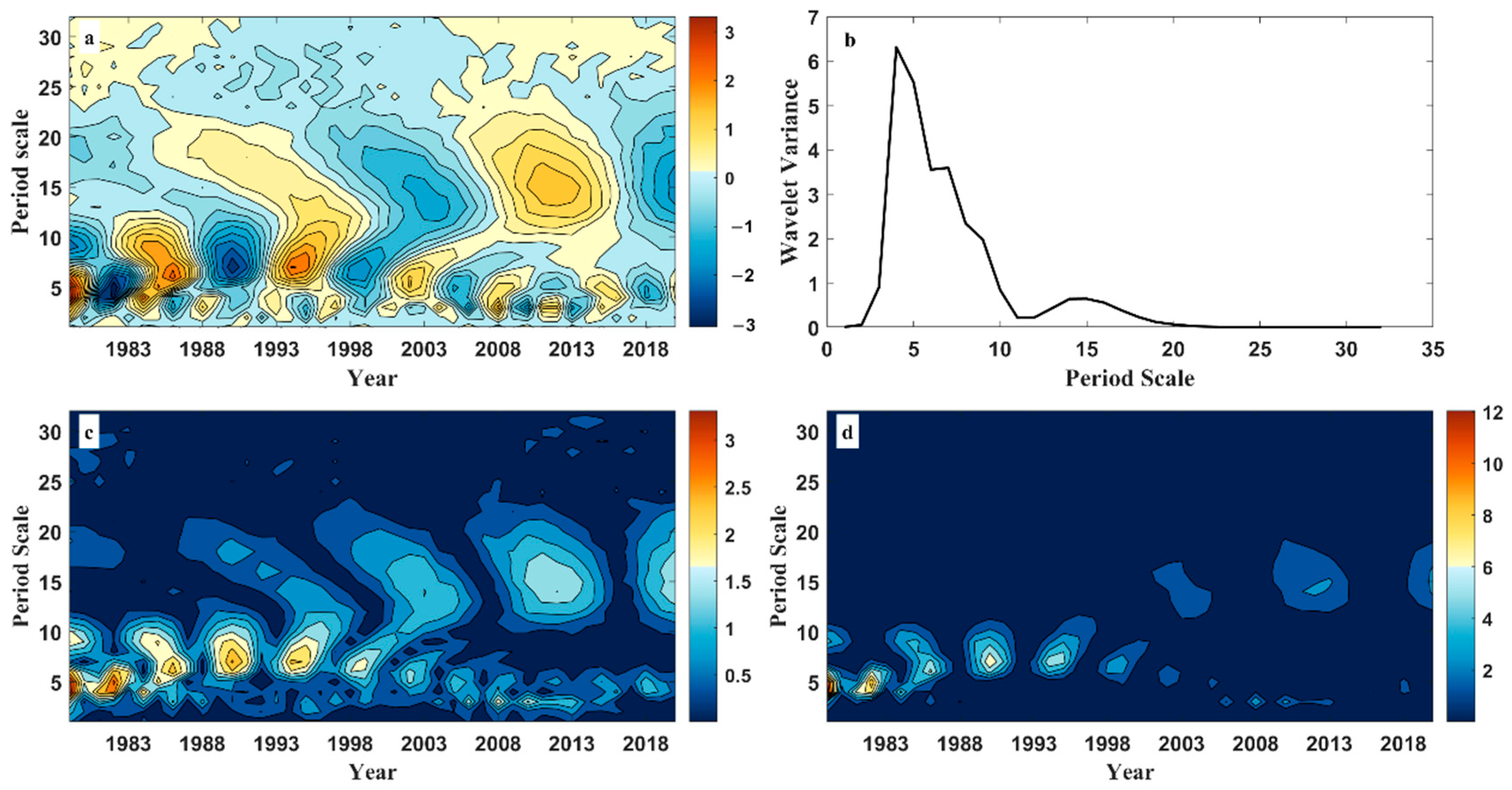
3.1.3. Wavelet Analysis of Multiple Time Scales

The continuous wavelet transform reflects the time-scale transformation characteristics of the signal itself. Under the condition of a certain scale, the change process of the wavelet coefficient with time reflects the periodic change of the element and its distribution in the time domain, and the wavelet variance can reflect the fluctuations of various scales (periods) contained in the time series and the characteristics of their strengths (energy levels) changing with the scales.
Figure 3 and Figure 4 show the wavelet analysis results of the occurrence frequency and cumulative days of blocking high in 42 extended winters from 1979 to 2021. It can be clearly seen from Figure 3a and Figure 4a that there are multi-scale features in the evolution process of the blocking high. In general, the evolution of the occurrence frequency and cumulative days of blocking high in extended winter mainly shows three oscillation periods, which are 3–4 years of periodic oscillation (corresponding to the wavelet transform scale of 2–5 years), 9–11 years of periodic oscillation (corresponding to the wavelet transform scale of 6–12 years) and the 18-year of periodic oscillation (corresponding to the wavelet transform scale of 10–27 years).
It can be seen from Figure 3b and Figure 4b that the maximum peak corresponds to the 4-year time scale, indicating that the periodic oscillation of this scale is the most prominent. Combining Figure 3c,d and Figure 4c,d, it can be analyzed that the energy on the 4-year time scale is the strongest and the cycle is the most significant, but its periodic changes are localized (1980s), and the energy on the 7–9-years time scale is weak, but the periodic distribution is more pronounced (1980s to early 2000s).

3.2. Circulation Characteristics of Blocking Highs in Ural Mountains in Extended Winter

Zhou [35] proposed in the statistical study of the blocking situation in the mid-latitude region of Asia that the blocking situation in the west of 100 degrees east longitude can be roughly divided into two types: the first type is that a mobile high-pressure ridge moves eastward and develops into a strong blocking situation, and the result of its development is often the formation of a strong high-pressure ridge that moves to the original location of the westerly jet (40°~60° N), making the south branch of the westerly jet tend to be straight; the second type is caused by the different moving speeds of the high-pressure ridge and the low-pressure trough. The final result of its development is the formation of closed high-pressure centers and low-pressure centers in the north and south, and causes a significant westerly branch. Most of the blocking high in the Ural Mountains belongs to the second category, which is characterized by long duration and less movement. Zhou [26] found that the Ural Mountains blocking high events would lead to low-temperature anomalies in Northeast, North, and Central China, and the strongest low-temperature anomalies occurred in northern Xinjiang.

Synthesis Analysis

Begin days are defined as the first days of each event in the 43 blocking high events, −2 days are the second days before the starting days, +2 days are the second days after the start days, +4 days are the fourth days after the starting days, and +6 days are the sixth days after the starting days.
In order to better analyze the circulation situation of the blocking high in the Ural Mountains region in extended winter, this paper conducts a synthetic analysis of 43 blocking events in the Ural Mountains region in extended winter from 1979 to 2021, and obtains the HGT anomaly field and the SAT anomaly field of −2 days, begin days, +2 days, +4 days and +6 days (Figure 5 and Figure 6). From the figure, we can see that the HGT anomaly field in the northern hemisphere in extended winter presents a relatively obvious “positive-negative-positive” staggered distribution, with three obvious positive and negative anomaly centers each. The centers of positive anomalies of HGT are located at 0°~60° W, 30°~90° E, 180°~120° W, and the centers of negative anomalies are located at 60°~120° W and 0°~30° E, 60°~120° E, respectively. The HGT anomaly map of −2 days shows that there is a positive HGT anomaly in the Ural Mountains area, the center of the positive anomaly is around 60° E, and its meridional span is large. At this time, the central intensity of the positive and negative HGT anomalies in the entire northern hemisphere is similar, and the range is also very close. In the SAT anomaly map, at −2 days, there is a positive SAT anomaly with weaker intensity and a smaller meridional span near the Barents Sea, while the region between Lake Balkhash and Lake Baikal has a negative SAT anomaly with a central strength slightly larger than the center of the positive anomaly.
By synthesizing the HGT anomalies and SAT anomalies of the beginning days of 43 blocking high events between 1979 and 2020, we can find that the central intensity of the HGT positive anomalies in the Ural Mountains area reaches a very high level, and its meridional span range is very large, reaching about 50 latitudes. The negative HGT anomaly over Western Europe weakened significantly. In terms of SAT, the central intensity and range of positive and negative anomalies are still increasing, and the longitude span is about 20 latitudes. From the HGT anomaly map on the third day of the blocking high process, we can see that the central intensity of the positive HGT anomaly in the Ural Mountains area remains high, showing an increasing trend, and the negative HGT anomaly over Western Europe is still weakened. From the SAT anomaly chart on the third day of the blocking high process, the positive anomaly near the Barents Sea is in a state of continuous growth. A relatively stable northwest-southeast dipole structure is formed. In the +4 days HGT anomaly map, the central intensity of the positive HGT anomaly in the Ural Mountains region has weakened compared with the previous one, and has a clear feature of moving westward. The negative HGT anomaly originally located in the Baikal region gradually moved eastward. In the +4 days SAT anomaly map, the northwest-southeast dipole structure also gradually expands westward. In the +6 days map, the central strength of the HGT positive anomalies in the Ural Mountains region has been significantly weakened, and the meridional span remains at around 40 latitudes. In addition, there is a small increase in the positive and negative center intensities on the remaining longitudes. On the SAT map, the central intensity and extent of the negative anomalies in the Eurasian mid-latitudes weakened slightly. It is worth noting that from the beginning of the blocking high, the southern side of the negative SAT anomaly gradually invaded the eastern part of China. In general, the spatial distribution of the HGT anomaly field is similar to the Eurasian Teleconnection Pattern (EU), a major circulation system in winter over the Eurasian region. The positive anomaly center is located in the Ural Mountains region, while the upper European region and the lower East Asian region of the Ural Mountains have significantly lower HGT. Combined with the SAT anomaly field, it is indicated that the changes in atmospheric circulation over the Ural Mountains may cause the European trough and the East Asian trough stronger by stimulating the EU-type teleconnection wave train, and thus have a significant influence on the weather over the Eurasian region [36].

3.3. The Effects of SST and SI on Blocking Highs in the Extended Wintertime Ural Mountains

Here, we take the average geopotential height anomaly of 500 hPa in the region (40°~70° N, 40°~80° E) from November to March as the Urals blocking high index (UBHI) in extended winter. First, the distribution of the correlation coefficient between the UBHI in extended winter and the SST (−10°~70° N, 0°~180° W) throughout the annual mean and four seasons mean was calculated (Figure 7). It can be seen from Figure 7 that whether it is the previous summer, the same winter, and the whole year, the UBHI in extended winter all showed a positive correlation with the SST in the North Atlantic sea area, and two positive correlations with sea areas (30°~60° N, 50°~75° W and 10°~30° N, 20°~90° W) passed the 95% significance test. This indicates that the positive SST anomaly in the North Atlantic sea area plays a very important role in the formation of the Ural blocking high in extended winter. In addition, we also noticed that in the Eastern Equatorial Pacific, the SST in the early spring, summer, autumn, and the whole year showed a weak positive correlation with the UBHI in extended winter, but in the same winter, it showed a weak negative correlation.
Therefore, in order to better analyze the impact of SST anomalies in key sea areas on the Ural Mountains blocking high, we calculated the SST anomaly indices NAI and EEPI in the North Atlantic sea area (one of significant positive correlation region, 30°~60° N, 50°~75° W) and the Eastern Equatorial Pacific sea area (the Niño 3.4 region, 5° N–5° S, 120° W–170° W) in winter. If the absolute value of the standardized index exceeds 0.5, it can be considered that the SST in this year is abnormally high/low. For the Eastern Equatorial Pacific, we selected a total of 14 high SST years and 12 low SST years. For the North Atlantic sea area, we selected a total of 10 high SST years and 11 low SST years. Figure 8 shows the synthetic results of the 500 hPa HGT field and 850 hPa wind field in high SST years and low SST years.
Figure 8a,d shows obvious zonal “− + − +” teleconnection wave trains, while Figure 8b,c show obvious zonal “+ − + −” teleconnection wave trains, with obvious abnormally high values located in the Ural Mountains region. Combined with the 850 hPa wind field, it can be seen that when the SST anomaly in the Eastern Equatorial Pacific was low in winter, there is a wide range of anticyclonic circulation anomalies in the wind field in the Ural Mountains, which will lead to the increase in atmospheric pressure in the region, showing a positive HGT anomaly, with the maximum anomaly value of 20 gpm, but it does not pass the significance test. Furthermore, when the SST is abnormally high in the North Atlantic sea area, there is a strong anticyclonic circulation anomaly in the Ural Mountains wind field, and the HGT is a positive anomaly, with the maximum anomaly reaching 30 gpm, which has passed the 95% significance test. In addition, we can see that the line connecting the centers of the anomalous circulation with alternating anticyclonic and cyclonic in Figure 8c is similar to the Eurasian wave train revealed by Wallace and Gutzler [37]. Therefore, the anomalously high SST in the North Atlantic sea area affects the atmospheric circulation over Eurasia by stimulating the Eurasian wave train [38], which makes the abnormal development and strengthening of the high-pressure ridge in the Ural Mountains, making it easier to form a blocking high.
In addition, in order to explore the impact of Arctic SI changes on the atmospheric circulation in the Ural Mountains, we also calculated the correlation coefficient between the UBHI in extended winter and the Arctic SI concentration throughout the annual mean and four seasons mean, as shown in Figure 9. We can find two significant correlation regions, the Barents-Kara Sea region and the Chukchi Sea region, both exhibiting negative correlations. Therefore, we calculated the Barents-Kara Sea (65° N–80° N, 30° E–100° E) and the Chukchi Sea (65° N–75° N,155° W–180° W) SI concentration anomaly index BKSI (Barents-Kara Sea Index) and CSI (Chukchi Sea Index), with plus or minus 0.5 standard deviations as the standard. For the Barents-Kara Sea, we selected a total of 10 high SI years and 11 low SI years. For the Chukchi sea, we selected a total of 11 high SI years and 11 low SI years. Figure 10 shows the synthetic results of the 500 hPa HGT field and 850 hPa wind field and in the high SI years and low SI years.
Figure 10b,d shows relatively consistent anomalous circulation patterns, both of which are positive anomalous large values in the Ural Mountains. At the same time, we can see that when the SI in the Barents-Kara Sea is abnormally low, there is a large range of anticyclonic cyclone field anomaly in 850 hPa over the Ural Mountains, and the 500 hPa HGT is a significant positive anomaly, which is conducive to the formation of blocking high. In addition, when the SI in the Chukchi Sea is abnormally low, the 850 hPa wind field in the Ural Mountains is also an anticyclonic anomaly, with a significant positive HGT but a relatively small intensity. It is noteworthy that when the SI in the Barents-Kara Sea and Chukchi Sea is abnormally less, the positive HGT anomaly position in the Ural Mountains is obviously westward.
Figure 11 shows the synthetic results of the STHF anomaly field in the low SI years. It can be clearly seen that both the Barents-Kara Sea and the Chukchi Sea have significantly upward STHF, that is, the atmosphere is heated. By calculating the longitude-altitude profile of the synthetic HGT and T in the Ural Mountains (Figure 12a,b), it is found that when the SI in the Barents-Kara Sea and the Chukchi Sea are abnormally low, there is a deep positive anomaly at 20° E–80° E, and the T of the entire atmosphere is relatively low. From the perspective of the latitude-altitude profile (Figure 12c,d), HGT and T have similar characteristics, which are bounded by 50° N and 60° N, respectively. Among them, the positive HGT anomaly mainly appears in the north of 50° N, and the positive T anomaly mainly appears in the north of 60° N, especially in the middle and upper troposphere and stratosphere. It can be seen that the reduction of SI in the two key regions in autumn may lead to warming over the Arctic regions, which in turn will lead to a weakening of the temperature gradient between the Arctic regions and the mid-latitude regions, resulting in a significant weakening of the westerly wind at the upper middle and high latitudes, thereby promoting the development and maintenance of the blocking high in the Ural Mountains.

4. Discussion

This study found that the frequency and duration of these occurrences in Ural Mountains blocking highs in the extended winters of 1979–2020 showed a downward trend, which is somewhat different from other previous results [39,40,41]. This difference may be due to the spatial resolution of the data and the definition of blocking high events. We defined the minimum duration of blocking high events as 5 days, which statistically excluded some blocking high events with a duration of 3–4 days (mainly occurring after the 21st century). In addition, many external forcing factors affect the formation of each blocking high in a particular region, including stratospheric explosive warming, SST anomalies, East Asian monsoon anomalies, and SI anomalies. This paper mainly focused on the key aspects of how SST and SI anomalies might affect a Ural Mountains blocking high in extended winter. Scientists agree that the El Niño–Southern Oscillation (ENSO) cycle that occurs in the Equatorial Eastern Pacific Ocean is a strong signal of air–sea interaction and is considered to be a critical factor underlying climate anomalies. This investigation revealed that an abnormally low SST in the Equatorial Eastern Pacific in winter, which corresponds to a La Niña event, was favorable for the formation of a blocking high in the Ural Mountains. One explanation may be the increased cyclone activity in the mid-latitudes of the northern hemisphere during La Niña year, in which the development of the dynamic and thermal forcing process is conducive to enhancing the forcing mechanism of the downstream ridge, leading to the transport of anticyclonic vorticity, thus favoring the formation of blocking highs [16]. At the same time, the higher SST in the North Atlantic sea area, which is adjacent to the Pacific Ocean, also has a significant impact on the formation of a blocking high in the Ural Mountains in extended winter. This phenomenon may be due to the typical “warm ocean/cold continent” temperature anomaly caused by high SST anomalies, along with resonance with topographic forcing that is beneficial to the occurrence and maintenance of blocking highs. Meanwhile, changes in atmospheric baroclinicity under different SST anomalies offer another reason for affecting the formation of a blocking high [42,43]. Han et al. found that the transient-eddy anomalies induced by the North Atlantic SST anomaly were a fundamental mechanism for the positive HGT anomaly over the Ural Mountains [38]. However, the interaction of the air–sea system is highly complex, and its possible influence pathways require further study.
In addition, the interannual variability of Arctic SI in autumn is very significant, and its anomalous changes have a crucial impact on the atmospheric circulation in extended winter. This investigation demonstrated that when the SI in the Barents-Kara Sea and the Chukchi Sea was abnormally low, the Ural Mountains blocking highs showed a significant westward shift, which might have been due to the amplification and upward propagation of the planetary wave in the upper troposphere. This troposphere caused the weakening of the stratospheric polar vortex and its transmission down to the troposphere offset the low-pressure anomaly formed by the tropospheric path in the high latitudes of the North Atlantic, resulting in a weakening of the North Atlantic westerly wind and guiding the Ural Mountains blocking highs to westward [44]. However, other studies have asserted that a quasi-steady Ural Mountains blocking high can change the surface fluxes of sensible and latent heat by increasing downward long-wave radiation, thereby triggering persistent severe SI melting [45,46]. Therefore, further research is needed on the cause-effect relationship and influencing mechanism between SI and the Ural Mountains blocking highs in extended winter.

5. Conclusions

Using the ERA-5 reanalysis data and the TM method, we selected blocking high events from 42 extended winter seasons between 1979 and 2020. From our analysis of the circulation characteristics and influencing factors of these blocking high events, we drew the following conclusions:
(1)
During the 42 extended winters from 1979 to 2020, a total of 43 blocking high events occurred in the Ural Mountains. The annual average number of blocking high events was 1.02, and the frequency of occurrence followed a downward trend. In addition, these blocking high events covered 312 days in total, with an annual average blocking period of 7.43 days. Interestingly, most of the short-lived blocking high events occurred after the 1990s. In addition, the frequency of occurrence and accumulated days of blocking highs in extended winter generally followed a 3–4 years oscillating cycle.
(2)
As a while, the 500 hPa anomaly field constituted a “positive-negative-positive” cross-distribution situation. As a blocking high developed, the intensity of the positive anomaly center in the Ural Mountains initially increased and then weakened, while the negative anomaly center on the east side showed the opposite pattern. On the SAT anomaly field, the central strength of the positive anomalies near the Barents Sea first increased and then decreased during the blocking process; however, the central strength and meridional span of the negative anomalies in the Eurasian mid-latitudes continued to increase until the edge reached the eastern part of China.
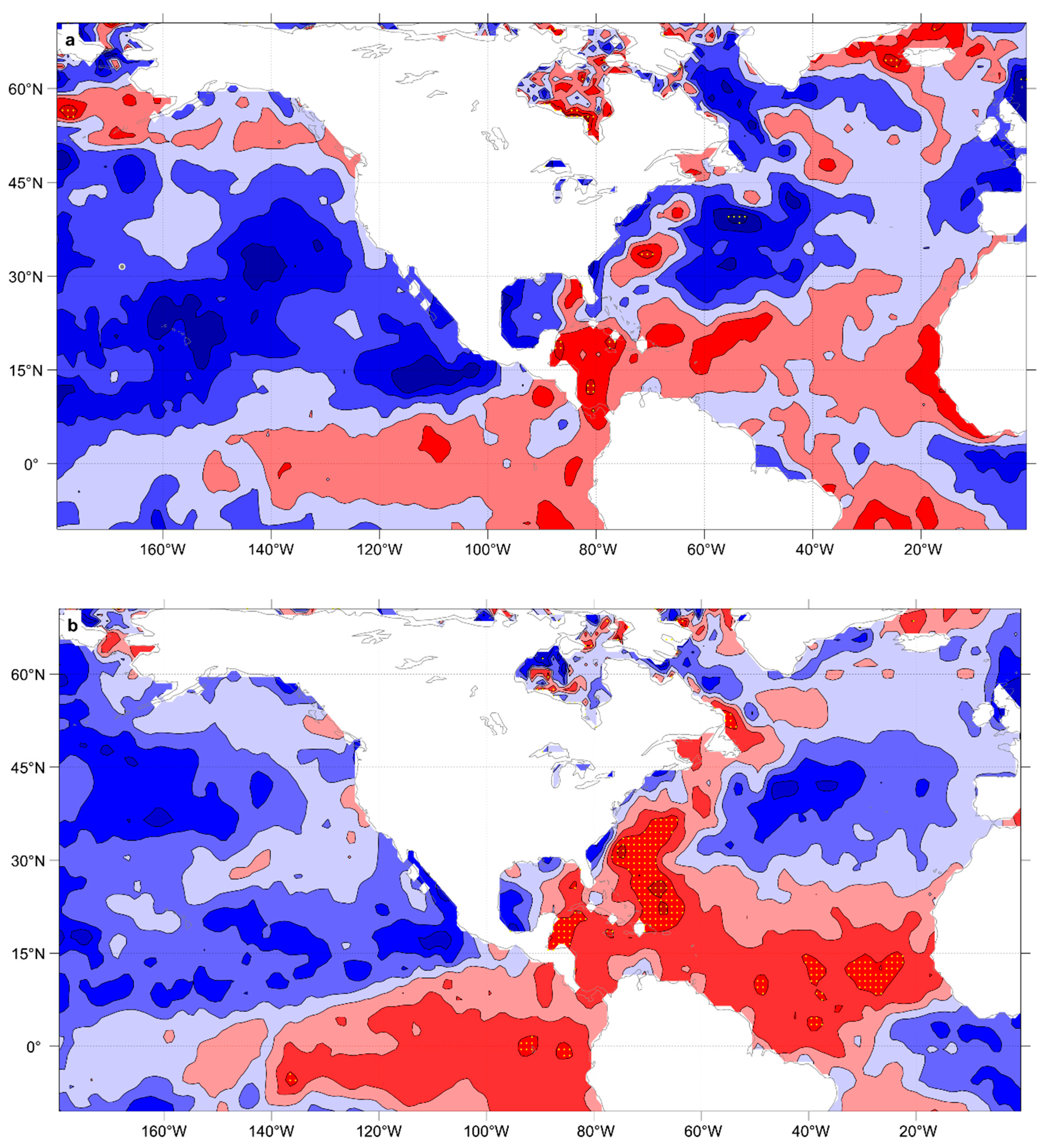
(3)
The abnormally high SST in the North Atlantic sea area and the abnormal reduction of SI in the Barents-Kara Sea and the Chukchi Sea in autumn had a significant impact on the formation of Ural Mountain blocking highs in extended winter. By comparison, the abnormally low SST in the Eastern Equatorial Pacific Ocean in winter also demonstrated a certain effect on Ural Mountains blocking highs, though the effect was not significant. In addition, the reduction of SI in the Barents-Kara Sea and the Chukchi Sea in autumn might also have led to a westward positioning of Ural Mountains blocking highs.

Author Contributions

Conceptualization, Y.L. and Y.Z.; methodology, Y.L.; software, Y.Z.; validation, Y.L. and Y.Z.; formal analysis, Y.L.; investigation, Y.L.; resources, Y.Z.; data curation, Y.L.; writing—original draft preparation, Y.L.; writing—review and editing, Y.Z.; visualization, Y.L.; supervision, Y.Z.; project administration, Y.Z.; funding acquisition, Y.Z. All authors have read and agreed to the published version of the manuscript.

Funding

This research was funded by the National Natural Science Foundation of China (Grant No. U1901215), the Marine Special Program of Jiangsu Province in China (JSZRHYKJ202007), and the Natural Scientific Foundation of Jiangsu Province (BK20181413).

Institutional Review Board Statement

Not applicable.

Informed Consent Statement

Not applicable.

Data Availability Statement

Not applicable.

Acknowledgments

The fifth generation ECMWF atmospheric reanalysis global climate dataset (ERA-5) during 1979–2021 are highly appreciated. This study was supported by the National Natural Science Foundation of China (Grant No. U1901215), the Marine Special Program of Jiangsu Province in China (JSZRHYKJ202007), and the Natural Scientific Foundation of Jiangsu Province (BK20181413).

Conflicts of Interest

The authors declare no conflict of interest.

References

  1. Li, Y.; Jin, R.H.; Wang, S.G. Statistical characteristics of blocking high in key regions affecting weather in China during 1950–2008. J. Lanzhou Univ. Nat. Sci. 2010, 46, 47–55. [Google Scholar]
  2. Masato, G.; Hoskins, B.J.; Woollings, T. Winter and summer Northern Hemisphere blocking in CMIP5 models. J. Clim. 2013, 26, 7044–7059. [Google Scholar] [CrossRef]
  3. Wu, J.; Diao, Y.; Zhuang, X.Z. The relationship between the Ural blocking in boreal winter and the East Asian winter monsoon. Clim. Environ. Res. 2016, 21, 577–585. [Google Scholar]
  4. Yang, G.; Kong, Q.; Mao, D.; Zhang, F.; Kang, Z.M.; Zong, Z.P. Analysis of the long lasting cryogenic freezing rain and snow weather in the beginning of 2008. Acta Meteorol. Sin. 2008, 66, 836–849. [Google Scholar]
  5. Shi, C.; Cai, W.; Jin, X. Modulation by transient waves of atmospheric longwave anomalies: Dynamic mechanism of the super cold wave in South China in the extremely strong El Nino of 2015/2016. Trans. Atmos. Sci. 2016, 39, 827–834. [Google Scholar]
  6. Li, Y.; Zhang, J.Y.; Lu, Y.; Zhu, J.; Feng, J. Characteristics of transient eddy fluxes during blocking highs associated with two cold events in China. Atmosphere 2019, 10, 235. [Google Scholar] [CrossRef] [Green Version]
  7. Davini, P.; Cagnazzo, C.; Anstey, J. A Blocking View of the Stratosphere-Troposphere Coupling; EGU General Assembly: Vienna, Austria, 2015. [Google Scholar]
  8. Oliveira, F.N.M.; Carvalho, L.M.V.; Ambrizzi, T. A new climatology for Southern Hemisphere blockings in the winter and the combined effect of ENSO and SAM phases. Int. J. Climatol. 2013, 34, 1676–1692. [Google Scholar] [CrossRef] [Green Version]
  9. Cheung, H.N.; Zhou, W.; Mok, H.Y.; Wu, M.C. Relationship between Ural-Siberian blocking and the East Asian winter monsoon in relation to the arctic oscillation and the El Nino-Southern oscillation. J. Clim. 2012, 25, 4242–4257. [Google Scholar] [CrossRef]
  10. Luo, D.; Xiao, Y.; Diao, Y.; Dai, A.; Franzke, C.L.; Simmonds, I. Impact of Ural blocking on winter warm arctic-cold Eurasian anomalies. Part II: The link to the North Atlantic Oscillation. J. Clim. 2016, 29, 3949–3971. [Google Scholar] [CrossRef]
  11. Cheung, H.N.; Zhou, W.; Shao, Y.; Chen, W.; Mok, H.Y.; Wu, M.C. Observational climatology and characteristics of wintertime atmospheric blocking over Ural-Siberia. Clim. Dyn. 2013, 41, 63–79. [Google Scholar]
  12. Tian, P.Y. Two Types of boreal wintertime blocking highs around Ural Mountains and their associated dynamic features. Master’s Thesis, Nanjing University of Information Science & Technology, Jiangsu, China, June 2019. [Google Scholar]
  13. Ma, X.Y.; Mu, M.; Dai, G.K.; Han, Z.; Li, C.; Jiang, Z. Influence of Arctic Sea Ice Concentration on Extended-Range Prediction of Strong and Long-Lasting Ural Blocking Events in Winter. J. Geophys. Res. Atmos. 2022, 5, e2021JD036282. [Google Scholar] [CrossRef]
  14. Lu, Y.; Li, X.; Li, Y.; Chen, Y. The Characteristics of Thermal and Momentum Transport During the Different Lifetimes of Ural Blocking Highs in Winter. Plateau Meteorol. 2022, 41, 671–683. [Google Scholar]
  15. Wang, S.Y.; Na, L.; Wang, P.; Zhu, X.W.; Li, X.; Ma, Y.; Zhang, W. Synergistic effects of ice and sea surface temperature on the precipitation abnormal in June in the central part of northwest China. Arid Land Geogr. 2021, 44, 63–72. [Google Scholar]
  16. Wiedenmann, J.M.; Lupo, A.R.; Mokhov, I.I.; Tikhonova, E.A. The climatology of blocking anticyclones for the Northern and Southern Hemispheres: Block Intensity as a Diagnostic. J. Clim. 2002, 15, 3459–3473. [Google Scholar] [CrossRef]
  17. Li, S.L. Impact of Northwest Atlantic SST Anomalies on the circulation over the Ural Mountains during early winter. J. Meteorol. Soc. Jpn. 2004, 82, 917–988. [Google Scholar] [CrossRef] [Green Version]
  18. Li, Y.; Lu, Y.; Wang, J.H.; Wang, Q. Effects of two types of ENSO events on the blockings in the Eurasian Region in winter. J. Lanzhou Univ. Nat. Sci. 2017, 53, 628–635. [Google Scholar]
  19. Overland, J.E.; Klaus, D.; Francis, J.A.; Hall, R.J.; Hanna, E.; Kim, S.-J.; Screen, J.A.; Shepherd, T.G.; Vihma, T. Nonlinear response of mid- latitude weather to the changing Arctic. Nat. Clim. Change 2016, 6, 992–999. [Google Scholar] [CrossRef] [Green Version]
  20. Feng, J.; Zhang, Y.; Tsou, J.; Wong, K. Analyzing variations in the association of Eurasian winter–spring snow water equivalent and autumn Arctic sea ice. Remote Sens. 2022, 14, 243. [Google Scholar] [CrossRef]
  21. Zhu, J.T.; Lu, Y.; Li, Y. Study on interdecadal variations of cold wave and genesis of atmospheric circulation in the Chinese Mainland from 1970 to 2019. J. Lanzhou Univ. (Nat. Sci.) 2022, 58, 337–355. [Google Scholar]
  22. Yao, Y.; Luo, D.H.; Dai, A.G.; Simmonds, I. Increased quasi stationary and persistence of winter Ural blocking and Eurasian extreme cold events in response to Arctic warming. Part I: Insights from observational analyses. J. Clim. 2017, 30, 3549–3568. [Google Scholar] [CrossRef]
  23. Woodruff, S.D.; Lubker, S.J.; Wolter, K.; Worley, S.J.; Elms, J.D. Comprehensive Ocean-Atmosphere Data Set (COADS) Release la: 1980-92. Earth Syst. Monit. 1993, 4, 1–8. [Google Scholar]
  24. Rayner, N.A. Global analyses of sea surface temperature, sea ice, and night marine air temperature since the late nineteenth century. J. Geophys. Res. Atmos. 2003, 108, 4407. [Google Scholar] [CrossRef] [Green Version]
  25. Shi, N.; Wang, Y. Energetics of Boreal Wintertime Blocking Highs around the Ural Mountains. J. Meteorol. Res. 2022, 36, 154–174. [Google Scholar] [CrossRef]
  26. Zhou, N. The spatial characters of blocking over Eurasia and its impact on temperature of China. J. Chengdu Univ. Inf. Technol. 2016, 31, 419–424. [Google Scholar]
  27. Lejenäs, H.; Økland, H. Characteristics of Northern Hemisphere blocking as determined from a long timeseries of observational data. Tellus 1983, 35, 350–362. [Google Scholar] [CrossRef]
  28. Tibaldi, S.; Molteni, F. On the operational predictability of blocking. Tellus 1990, 42, 343–365. [Google Scholar] [CrossRef] [Green Version]
  29. Morlet, J.; Arens, G.; Fourgeau, E.; Giard, D. Wave propagation and sampling theory—Part II: Sampling theory and complex waves. Geophysics 1982, 47, 222–236. [Google Scholar] [CrossRef] [Green Version]
  30. Le, T.P. Use of the Morlet mother wavelet in the frequency-scale domain decomposition technique for the modal identification of ambient vibration responses. Mech. Syst. Signal Process. 2017, 95, 488–505. [Google Scholar] [CrossRef]
  31. Chong, K.L.; Huang, Y.F.; Koo, C.H.; Ahmed, A.N.; El-Shafie, A. Spatiotemporal variability analysis of standardized precipitation indexed droughts using wavelet transform. J. Hydrol. 2021, 605, 2–19. [Google Scholar] [CrossRef]
  32. Zhang, S.W.; Lei, Y.J.; Feng, Y.Q. Application of Matlab in Time Series Analysis; Xidian University Press: Xi’an, China, 2007. [Google Scholar]
  33. Shi, X.J.; Zhi, X.F. Statistical characteristics of blockings in Eurasia from 1950 to 2004. Trans. Atmos. Sci. 2007, 30, 338–344. [Google Scholar]
  34. Ye, P.L.; Li, Y.; Wang, S.G.; Wang, X.J.; Shang, K.Z. Variation characteristics of different atmospheric blockings and their impact on temperature over the Northern Hemisphere. J. Lanzhou Univ. (Nat. Sci.) 2015, 51, 639–651. [Google Scholar]
  35. Zhou, X.P. Statistical investigation on the blocking situations over Asia. Acta Meteorol. Sin. 1957, 1, 77–87. [Google Scholar]
  36. Lu, Y. Study on the change characteristics and mechanism of Ural Blocking Highs under the global warming. Doctor’s Thesis, Lanzhou University, Lanzhou, China, June 2022. [Google Scholar]
  37. Wallace, J.M.; Gutzler, D.S. Teleconnections in the Geopotential Height Field during the Northern Hemisphere Winter. Mon. Weather Rev. 1981, 109, 784–812. [Google Scholar] [CrossRef]
  38. Han, Z.; Li, S.; Mu, M. The Role of Warm North Atlantic SST in the Formation of Positive Height Anomalies over the Ural Mountains during January 2008. Adv. Atmos. Sci. 2011, 28, 246–256. [Google Scholar] [CrossRef]
  39. Luo, B.; Luo, D.; Dai, A.; Simmonds, I.; Wu, L. Decadal variability of winter warm Arctic-cold Eurasia dipole patterns modulated by Pacific Decadal Oscillation and Atlantic Multidecadal Oscillation. Earth’s Future 2022, 10, e2021EF002351. [Google Scholar] [CrossRef]
  40. Luo, B.; Luo, D.; Dai, A.; Simmonds, I.; Wu, L. The modulation of Interdecadal Pacific Oscillation and Atlantic Multidecadal Oscillation on winter Eurasian cold anomaly via the Ural blocking change. Clim. Dyn. 2022, 59, 127–150. [Google Scholar] [CrossRef]
  41. Luo, B.; Wu, L.; Luo, D.; Dai, A.; Simmonds, I. The winter midlatitude-Arctic interaction: Effects of North Atlantic SST and high-latitude blocking on Arctic sea ice and Eurasian cooling. Clim. Dyn. 2019, 52, 2981–3004. [Google Scholar] [CrossRef]
  42. Shabbar, A.; Huang, J.; Higuchi, K. The relationship between the wintertime north Atlantic oscillation and blocking episodes in the north Atlantic. Int. J. Climatol. 2001, 21, 355–369. [Google Scholar] [CrossRef]
  43. Wan, H.; Luo, D.H. The relationship between wintertime blockings in the North Hemisphere and North Atlantic Oscillation. J. Trop. Meteorol. 2009, 25, 615–620. [Google Scholar]
  44. Chen, X.; Luo, D.; Wu, Y.; Dunn-Sigouin, E.; Lu, J. Nonlinear response of atmospheric blocking to early winter Barents–Kara Seas warming: An idealized model study. J. Clim. 2021, 34, 2367–2383. [Google Scholar] [CrossRef]
  45. Chen, X.; Luo, D.; Feldstein, S.B.; Lee, S. Impact of winter Ural blocking on Arctic sea ice: Short-time variability. J. Clim. 2018, 31, 2267–2282. [Google Scholar] [CrossRef]
  46. Gong, T.; Luo, D. Ural blocking as an amplifier of the Arctic sea ice decline in winter. J. Clim. 2017, 30, 2639–2654. [Google Scholar] [CrossRef]
Figure 1. (a) the interannual variation of the frequency of blocking high (unit: time), and (b) the number of blocking high occurring every month (unit: time) in the Ural Mountains.
Atmosphere 14 00129 g001
Figure 2. (a) The cumulative days of blocking high varied annually (unit: day), and (b) the number of times of blocking high in different lifetime (unit: times) in the Ural Mountains region.
Atmosphere 14 00129 g002
Figure 3. Wavelet analysis results of the occurrence frequency of Ural Mountains blocking high in extended winter ((a): real part of wavelet coefficient; (b): wavelet variance; (c): modulus of wavelet coefficient; (d): modulus square of wavelet coefficient).
Atmosphere 14 00129 g003
Figure 4. Wavelet analysis results of the cumulative days of Ural Mountains blocking high in extended winter ((a): real part of wavelet coefficient; (b): wavelet variance; (c): modulus of wavelet coefficient; (d): modulus square of wavelet coefficient).
Atmosphere 14 00129 g004
Figure 5. Synthetic analysis of the 500 hPa HGT anomaly field before and after the occurrence of the Ural Mountains blocking highs in the extended winter of 1979–2020 (the red line indicates a positive anomaly value, and the blue line indicates a negative anomaly value, grey shaded area through the test of significance of 95%).
Atmosphere 14 00129 g005
Figure 6. Synthetic analysis of the SAT anomaly field before and after the occurrence of the Ural Mountains blocking highs in the extended winter of 1979–2020 (the red line indicates a positive anomaly value, and the blue line indicates a negative anomaly value, grey shaded area through the test of significance of 95%).
Atmosphere 14 00129 g006
Figure 7. The correlation coefficient between the UBHI in extended winter and SST throughout the four seasons mean ((a): spring; (b): summer; (c): autumn; (d): winter) and annual mean (e) (dotted area through the test of significance of 95%).
Atmosphere 14 00129 g007aAtmosphere 14 00129 g007bAtmosphere 14 00129 g007c
Figure 8. Synthetic analysis of the 500 hPa HGT anomaly field (contour lines, unit: gpm) and 850 hPa wind anomaly field (arrows, unit: m/s) (high (a)/low (b) SST years in the Eastern Equatorial Pacific sea area; high (c)/low (d) SST years in the North Atlantic sea area) (red contour lines mean positive HGT anomaly, blue contour lines mean negative HGT anomaly, the contour lines interval is 5 gpm, grey shaded area through the test of significance of 95%).
Atmosphere 14 00129 g008
Figure 9. The correlation coefficient between the UBHI in extended winter and SI throughout the four seasons mean ((a): spring; (b): summer; (c): autumn; (d): winter) and annual mean (e) (red shaded area means positive correlation coefficient, blue shaded area means negative correlation coefficient, the absolute value of the correlation coefficient of shaded area is greater than 0.3 and through the test of significance of 95%).
Atmosphere 14 00129 g009
Figure 10. Synthetic analysis of the 500 hPa HGT anomaly field (contour lines, unit: gpm) and 850 hPa wind anomaly field (arrows, unit: m/s) (high (a)/low (b) SI years in the Barents-Kara Sea region; high (c)/low (d) SI years in the Chukchi Sea region) (red contour lines mean positive HGT anomaly, blue contour lines mean negative HGT anomaly, the contour lines interval is 5 gpm, grey shaded area through the test of significance of 95%).
Atmosphere 14 00129 g010
Figure 11. Synthetic analysis of the STHF anomaly field (low (a) SI years in the Barents-Kara Sea region; low (b) SI years in the Chukchi Sea region) (shaded area through the test of significance of 95%).
Atmosphere 14 00129 g011
Figure 12. Longitude-altitude profile (a,b) and latitude-altitude profile (c,d) of the synthetic HGT(shadings, unit: gpm) and T(contour lines, unit: °C) anomaly field (low (a,c) SI years in the Barents-Kara Sea region; low (b,d) SI years in the Chukchi Sea region) (black solid contour lines mean positive T anomaly, black dashed contour lines mean negative T anomaly, the contour lines interval is 0.2 °C).
Atmosphere 14 00129 g012
Disclaimer/Publisher’s Note: The statements, opinions and data contained in all publications are solely those of the individual author(s) and contributor(s) and not of MDPI and/or the editor(s). MDPI and/or the editor(s) disclaim responsibility for any injury to people or property resulting from any ideas, methods, instructions or products referred to in the content.

