Article

Temporal and Spatial Modal Analysis and Prediction of Tropospheric CO Concentration over the World and East Asia

1
School of Electrical and Information Engineering, School of Computer Science and Engineering, Anhui University of Science and Technology, Huainan 232001, China
2
School of Electrical and Photoelectronic Engineering, West Anhui University, Lu’an 237012, China
3
School of Internet, Anhui University, Hefei 230039, China
*
Authors to whom correspondence should be addressed.
Atmosphere 2022, 13(9), 1476; https://doi.org/10.3390/atmos13091476
Submission received: 17 August 2022 / Revised: 5 September 2022 / Accepted: 8 September 2022 / Published: 12 September 2022

Abstract

:
Spatiotemporal modal analysis and prediction of tropospheric atmospheric CO concentration in the world and East Asia from 2002 to 2021 using the inversion data of airs sounder. The results show that: The CO concentration in the northern hemisphere is higher than that in the southern hemisphere; from the upper troposphere to the lower troposphere, the CO concentration changes from “ “ to “√”; the fluctuation range of near surface CO concentration in the northern hemisphere is relatively intense, and the fluctuation range in the southern hemisphere is relatively small. Using MK, Sen slope estimation, and EOF analysis, it is found that CO concentration in the convective middle layer tends to decline in more than 90% of the global area, and the decline rate in the northern hemisphere is significantly higher than that in the southern hemisphere. In East Asia, the CO concentration in the lower tropospheric marine area is significantly lower than that in the land area. The average concentration and decline rate of CO in East Asia is always higher than that in the world; the CO concentration in East Asia is the highest in spring and winter in the lower troposphere; and the CO concentration in East Asia is lower in the northeast and higher in the southeast in the upper troposphere in spring, autumn, and winter, and higher in the northeast and Central Plains in summer. Compared with the three-exponential smoothing model, the prediction error of the VMD-LSTM hybrid model for atmospheric CO concentration is significantly reduced, which indicates that the improved neural network prediction model has higher prediction accuracy. The factors affecting the change of tropospheric CO concentration are not only affected by the ground factors, but also related to indirect factors such as water vapor, methane, and atmospheric temperature in the atmosphere.

1. Introduction

Carbon monoxide (CO) plays a very important role in atmospheric environmental pollutants. It is one of the main gases of atmospheric pollution sources and is also the gas with the highest carbon content in the atmosphere—except carbon dioxide and methane. It acts as an important oxidant in the troposphere when chemical reactions occur, and plays an important role in the global carbon cycle [1,2,3,4]. Since CO is the main sink of OH free radicals in the atmosphere, the effect of CO on global climate, mainly through the consumption of OH radicals (about 60%), can be from the impact of the concentration distribution of greenhouse gases in the atmosphere (CO2, CH4, and O3)—with both a global or regional influence “greenhouse effect”—which will also have a great impact on the chemical reactions of free particles in the atmosphere and seriously affect global climate change [5,6,7,8].
CO mainly comes from human activities and the natural ecological environment [9]. Human factors include the metallurgical industry, coal combustion, mine explosions, exhaust emissions from some vehicles (cars), metabolism and body combustion of some animals, etc; the natural factors include frequent earthquakes and volcanic eruptions in many areas of the island, as well as forest fires. In recent years, the frequent increase of human industrial activities, which has seriously affected the global CO budget and climate change has made the research on the temporal and spatial distribution of the CO concentration of great significance. Given that ground CO observation data will be affected by the uneven distribution of stations and human factors, satellite detection technology with omnidirectional, stable, and long time-series can be used to analyze air pollutants [10,11] At present, many scholars around the world have studied the spatial and temporal distribution of global or regional CO concentration through data statistics, ground observation, and satellite remote sensing technology. Since the late 1960s and early 1970s, many scholars have begun to study the distribution of CO in the troposphere. First, Robbins R C et al. [12], Seiler et al. [13], and Fishman J et al. [14] analyzed the total amount of carbon monoxide and ozone columns in the world in terms of latitude and vertical height; the results showed that the content of these pollutants in the northern hemisphere is always higher than that in the southern hemisphere, and the change in CO concentration is seasonal. The highest season of CO concentration in the northern hemisphere is spring, while the highest season of CO concentration in the southern hemisphere is autumn, and the change is more obvious in the northern hemisphere. At present, there are relatively few ground-based observation stations in the world, so many scholars at home and abroad are using satellite remote sensing data to analyze the spatial–temporal distribution and impact of CO concentration around the world. Tang born et al. [15] used SCIAMACHY column total data to study the influencing factors of global and regional distribution. Worden H M et al. [16] used a MOPITT space instrument to analyze tropospheric CO after 2000, and the decline trend in the United States, Europe, and East Asia from 2000 to 2010 was very significant. Jindal P et al. [17] analyzed the temporal and spatial characteristics of atmospheric temperature, water vapor, ozone, methane, and carbon monoxide in major Indian cities from 2003 to 2012 by using Aqua-AIRS products and found that the total amount of methane columns in all studied cities showed an upward trend, but the total amount of carbon monoxide columns showed an obvious downward trend. It is also the focus of many experts and scholars in the world to study the spatial–temporal variation of atmospheric CO in East Asia, where the economy is developing rapidly and the industry is already developed. Peng L et al. [18] calculated the total amount of CO column over the land of China by using satellite model inversion. Streets D G et al. [19] calculated the concentration of CO in China and revised the emissions by using sciamachy data. Tohjima Y et al. [20], Yumimoto K et al. [21], Jiang Z et al. [22], and Zheng B et al. [23] analyzed CO emissions in East Asia and found that human activities were the main source of CO in East Asia. The increase of CO emissions in East Asia was mainly caused by the increasing human base. According to MEIC data analysis, China’s CO emission reduction accounted for 84% of the global total emission reduction from 2005 to 2016.
Although many scholars have studied the temporal and spatial distribution of CO concentration, most of them have studied the total amount of CO column in the global region. Atmospheric CO plays different roles and changes in different atmospheres. Given that the troposphere is the level that has the closest contact with human beings, the troposphere is also the level that has the most drastic changes. Affected by the chemical properties of CO itself, analyzing the changes of atmospheric CO concentration at different levels in the troposphere will not only have a significant impact on the study of complex and changeable tropospheric greenhouse gases, it also provides valuable reference materials for scholars studying the Earth’s atmosphere system. The total amount of CO column mainly reflects the overall change of each region, and it is difficult to reflect the space-time distribution characteristics of atmospheric CO at each level. Therefore, it is necessary to evaluate the CO concentration at different levels of the atmosphere.
Few studies have studied the temporal and spatial variation trend of CO concentration in different atmospheric pressure layers in the troposphere in East Asia, where the economy has developed rapidly, especially during the past decade. In this paper, the spatial–temporal characteristics of the global and East Asian regions are analyzed by using the CO data of different tropospheric pressure layers that were retrieved by the long time-series satellite detector, AIRS, and the spatial–temporal modal analysis and trend prediction of the global and East Asian CO concentration changes are carried out by using the meteorological research algorithms, such as trend testing and modal prediction, which are commonly used in climate analysis methods.

2. Data Sources and Analysis Methods

2.1. Data Sources

AIRS (Atmospheric Infrared Sounder), a satellite detector mounted on the Earth observation system (EOS), was launched on 4 May 2002, and its detection wavelength is 4–120 μm. There are 2378 spectral channels with a resolution of 1200 (λ/Δλ), and it mainly collects atmospheric parameters such as atmospheric temperature, pressure, water vapor, methane, ozone, and CO. The retrieved standard CO data is from 1000 hPa to 1 hpa, with a total of 24 pressure layers and a longitude and latitude resolution of 1° × 1° for a monthly average dataset—the data storage format is an HDF file, which can be found on the official website http://old-cdc.cma.gov.cn/satellite/subject.jsp?product=AIRS Get data [24,25,26], (accessed on 6 June 2022).
Zhang L et al. [27] used six ground stations at different locations and elevations, which were used to verify the spectrometer for atmospheric charting (SCIAMACHY), measurement of pollution in the tropism (MOPITT), and AIRS detectors, respectively. The research results show that these three kinds of instruments can reflect the spatial distribution of CO well, and MOPITT and AIRS show high accuracy, and the correlation coefficient with the detected CO concentration on the ground is mostly more than 0.70. In conclusion, the carbon monoxide data obtained by using the AIRS detector has high reliability when analyzing the space-time characteristics.

2.2. Research Methods

2.2.1. Pearson Correlation Coefficient

A Pearson correlation coefficient is mainly used to measure the closeness of the relationship between two variables, and R is usually used to represent the correlation coefficient of two groups of variables. In this paper, Pearson’s correlation coefficient is used to measure the correlation between base station CO data and satellite CO data. At the same time, the correlation test was also carried out between near-surface CO data and water vapor, atmospheric temperature, and methane data. The specific calculation formula is as follows (the calculation formula takes satellite CO data set and satellite methane data as examples):
x i = ( x 1 , x 2 , , x n ) means a long time-series set of CO data, and y i = ( y 1 , y 2 , , y n ) means a long time-series set of methane data.
R = n i = 1 n x i y i i = 1 n x i i = 1 n y i n i = 1 n x i 2 ( i = 1 n x i ) 2 n i = 1 n y i 2 ( i = 1 n y i ) 2 ( | R | 1 )
When R > 0, which means the CO data is positively correlated with methane data, the methane concentration increases; when R < 0, which means the CO data is negatively correlated with methane data, the CO concentration decreases with the increase of methane concentration; and when R = 0, said CO and methane data have wireless sexual relationships, in which the greater the absolute value of R , the stronger the correlation between the two sets of data.

2.2.2. Linear Inclination Rate

The linear tilt rate is mainly used to judge the growth rate of variables with years. In this paper, the linear tilt rate was used to calculate the annual change rate of different pressure layers in the world and East Asia from 2003 to 2021. The specific formula is as follows:
x i represents a variable with CO data amount of N, t i represents the corresponding time of x i , and the established linear regression equation is as follows:
x i = b + k t i
In the formula, k is the slope, b is the regression constant, constant b and slope k are estimated by the least square method, and the formula is:
k = i = 1 n x i t i 1 n ( i = 1 n x i ) ( i = 1 n t i ) i = 1 n t i 2 1 n ( i = 1 n t i ) 2
b = x ¯ k t ¯
The sign of slope k represents the trend of CO. When k < 0, the CO concentration shows a downward trend in this period; when k > 0, the CO concentration shows an upward trend in this period. The absolute value of k can measure the degree of the upward or downward trend of CO concentration change in this period.

2.2.3. Sen Slope Estimation

The linear tilt rate is mainly used to judge the growth rate of variables with years. In this paper, the linear tilt rate was used to calculate the annual change rate of different pressure layers in the world and East Asia from 2003 to 2021. The specific formula is as follows:
The Sen slope estimation method is a robust trend calculation method of non-parametric statistics proposed by Sen in 1968. This method is insensitive to abnormal data and is superior to other regression models [28] for trend analysis of long-term series. It is often used with an MK trend test, and the specific calculation formula is as follows:
β is the Sen slope value of the long time series of CO, which represents the average change rate and trend of the series. If β > 0, it indicates that the CO concentration shows an upward trend over time. If β < 0, it indicates that the CO concentration decreases with time. For CO time-series, x i = ( x 1 , x 2 , , x n ) , the Sen slope calculation formula is as follows:
β = Median ( x j x i j i ) , j > i
In this formula is the median function.

2.2.4. Mann-Kendall (MK) Trend Test

The Mann-Kendall trend analysis method is widely used in meteorology and hydrology. The main purpose of this method is to evaluate whether there is an upward or downward monotonic trend in the dataset [29]. The MK calculation formula is as follows:
For CO time-series, x i = ( x 1 , x 2 , , x n ) , n 0 defines statistic S :
S = i = 1 n 1 j = i + 1 n sgn ( x j x i )
sgn ( θ ) is a sign function. If θ is less than 0, the value is −1; if θ is equal to 0, the value is 0; and if θ is greater than 0, the value is 1. Z is obtained by standardizing S , and the Z value is used for the significance test. The formula is as follows:
V = n ( n 1 ) ( 2 n + 5 ) 18
Z = { S 1 V S > 0 0 S = 0 S + 1 V S < 0
In this paper, Z > 0 can indicate that the carbon monoxide concentration presents an upward trend, otherwise it presents a downward trend. Given significance level α , | Z | Z 1 α 2 , which shows the trend is not significant. On the contrary, the trend is significant.

2.2.5. Empirical Orthogonal Decomposition Method

The empirical orthogonal function analysis (EOF) is often used to analyze the spatial and temporal changes of a single field. This analysis method mainly decomposes the variable field that changes with time into a spatial function part that does not change with time and a time part that only depends on time [30]. EOF represents the modal space part, and PC represents the change of the corresponding spatial mode with time. In this paper, the CO concentration matrix X is decomposed into spatial modes and time-series, that is X = E O F m n P C m n , where m is the global grid number of the CO longitude and latitude and n is the length of the CO time-series. Therefore, when using EOF to analyze the spatiotemporal variation characteristics of global CO, it is necessary to combine the spatial function and time coefficient for analysis and research.

2.2.6. Three-Exponential Smoothing Model Prediction

Exponential smoothing is done by observing the recent data and by giving it a higher weight compared to the weight given to the earlier data by low, weighting geometric diminishing at a constant rate, which is done to the recent training data that will play a role in the forecast analysis in the future, especially when the change in the single index mathematical model is suitable for a smooth time-series, and when the mathematical model is suitable for a double index and has a trend in the time-series data. The three-index model is suitable for time-series data with a trend and periodicity, and is very suitable for the prediction of seasonal CO concentration trend changes in this paper.

2.2.7. Introduction to the Basic Principles of VMD

VMD is a signal processing and noise reduction method proposed based on time-frequency analysis. By calculating the Hilbert transform of each modal component, and then estimating each component using Gaussian smoothing, the sum of the modal bandwidths can be minimized. The specific formula is as follows:
{ min { u k } , { w k } { k = 1 K | | ϑ t [ ( δ ( t ) + j π t ) u k ( t ) ] e j w k t | | 2 2 } s . t . k K u k = f
where K is the number of set modal components, u k w k are the kth modal component and the center frequency of the decomposition, and F is the original sequence.
In order to obtain the optimal solution for Formula (9), the constrained variational problem is changed to the unconstrained variational problem, and the Lagrange function needs to be used:
L ( { u k } , { w k } , λ ) = α k = 1 K | | ϑ t [ ( δ ( t ) + j π t ) u k ( t ) ] e j w k t | | 2 2 + | | x ( t ) k = 1 K u k ( t ) | | 2 2 + λ ( t ) , x ( t ) k = 1 K u k ( t )
where α is the penalty factor of the quadratic term and λ is the Lagrange multiplier.
Finally, VMD uses the alternating multiplier direction algorithm to obtain the optimal solution for Formula (9) [31].

2.2.8. Introduction to the Basic Principles of LSTM

LSTM is a variant structure proposed to solve the gradient disappearance caused by the long-term dependence of recurrent neural networks, which has achieved excellent results in time-series prediction [32,33]. The specific architecture is shown in Figure 1.
Ct in the figure represents the cell state; h t is hidden; i , f , and o are the input gate, forgetting gate, and output gate, respectively; x t is a single cell input; c t 1 is the last cell state; and h t 1 is the hidden state of the previous cell. The specific calculation formula is as follows:
f t = s i g m o i d ( W f [ h t 1 , x t ] + b f )
i t = s i g m o i d ( W i [ h t 1 , x t ] + b i )
o t = s i g m o i d ( W o [ h t 1 , x t ] + b o )
z t = tanh ( W z [ h t 1 , x t ] + b z )
c t = ( c t 1 f t ) ( Z t i t )
h t = tanh ( c t ) o t

2.2.9. Evaluating Indicator

1. The mean absolute error (MAE)—the loss value of absolute error—is the mean of the error between the predicted value and the actual value, which can better represent the measurement standard between the predicted value and the real value. The calculation formula is as follows, where n is the number of samples, y i is the actual value of CO concentration, and h ( x i ) is the model predicted value:
MAE ( X , h ) = 1 n i = 1 n | h ( x i ) y i |
2. The root mean square error ( R M S E ), which represents the standard deviation of the deviation between the real value and the predicted value, is calculated as follows:
R M S E = 1 n i = 1 n ( y i h ( x i ) ) 2
3. The coefficient ( ) is determined to represent the generalization ability of the model, and the values range from 0 to 1. The larger the value is, the better the prediction effect of the model. When the value is 1, the model has the best performance. The calculation formula is as follows:
y ¯ = 1 n i = 1 n y i
R 2 = 1 i = 1 n ( h ( x i ) y i ) 2 i = 1 n ( y i y ¯ ) 2

3. Temporal and Spatial Distribution Characteristics of Global CO

3.1. Spatial Variation Characteristics of CO in Different Pressure Layers of Troposphere

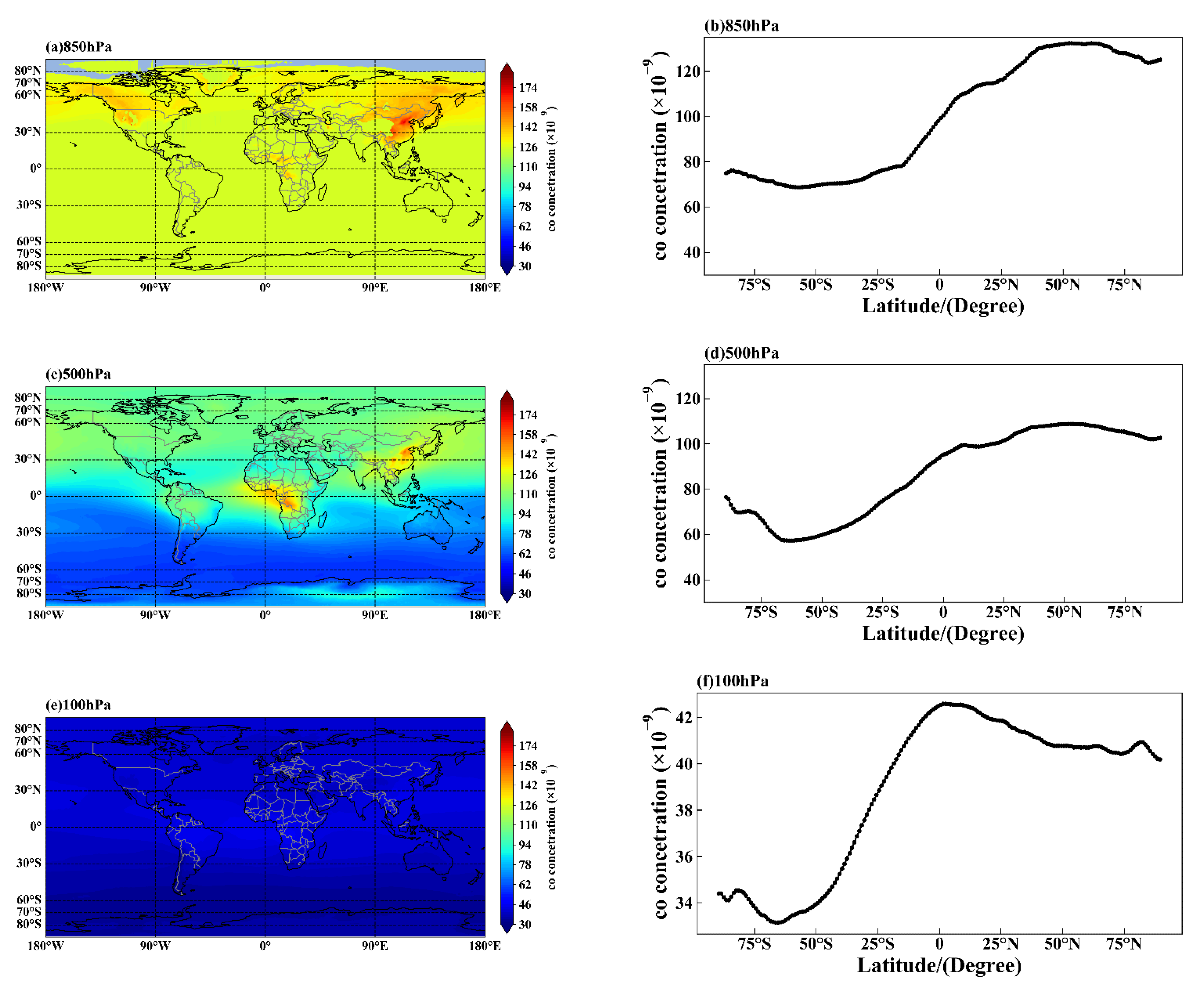
Figure 2 shows the spatial distribution and latitude variation trend of global CO concentration when the atmospheric pressure layer is 850 hPa, 500 hPa, and 100 hPa, respectively. The selected period is the average CO concentration from 2003 to 2020. Figure 2a,b shows the CO concentration data in the lower troposphere close to the ground (850 hPa). It can be seen from Figure 2b that the latitude variation curve of CO concentration in this atmospheric pressure layer shows a “spoon”-type change. The CO concentration in the southern hemisphere is lower than that in the northern hemisphere as a whole, mainly because the CO concentration is mainly influenced by human activities and surface organisms (photosynthesis)—since the majority of sea areas are in the southern hemisphere and there is more land distribution in the northern hemisphere; furthermore, human activities and vegetation growth are mainly concentrated in the northern hemisphere. Therefore, compared with the southern hemisphere, the spatial distribution of CO concentration in the northern hemisphere is scattered and fluctuates greatly. It can be seen from Figure 2a that the CO concentration in East Asia, North America, and parts of Africa is generally higher. The regions with high CO concentrations in the world are mainly concentrated in the East Asian mainland, which may be because the CO concentration in China is generally higher than that in other regions due to the rapid economic development and heavy industry activities in China over the past 40 years. Figure 2c,d shows the CO concentration in the middle troposphere (500 hPa). The change pattern of this atmospheric pressure layer is similar to that of the lower troposphere. Under the influence of land (human activities and surface organisms) and ocean, the CO concentration in the northern hemisphere is significantly higher than that in the southern hemisphere, and the overall concentration in this layer is relatively low. However, in addition to the East Asian continent, the high-value area also increased in central Africa. The reason why central Africa forms a high-value area in the middle troposphere may be caused by the climate, geographical location, and tropospheric characteristics. Central Africa belongs to a tropical climate and tropical rainforest climate and is in a high-temperature state all year round. Therefore, atmospheric CO in the lower troposphere is easy to react with OH ions in the air, resulting in low CO in the lower troposphere, and because tropospheric temperature gradually decreases with the increase of altitude. Moreover, most of northern Africa is a plateau, however, central Africa is located in a basin, so as the height increases, CO reacts less with free factors in the air and CO from the plateau around the plain will also flow to the central region, thus forming a high-value area of CO concentration in the central troposphere. Figure 2e,f shows the perennial average distribution of CO in the upper troposphere (100 hPa). Combined with Figure 2a,c,e, it can be seen that with the gradual decrease of the atmospheric pressure layer, the spatial variation of CO concentration shows a great change. When the atmospheric pressure layer is 100 hPa, the global CO concentration is generally at a low value. It is difficult to see the global CO concentration distribution from the spatial distribution map, so it can only be analyzed from the latitude change curve. For example, Figure 2f is the tropospheric latitude change map of 100 hPa. Given that it can be seen from Figure 2e, the CO concentration in the upper troposphere is at a very low value compared with the CO concentration in the lower troposphere. When drawing the latitude change map of the upper troposphere, the maximum and minimum values of CO concentration in the upper troposphere are selected as the critical values for controlling the concentration range of the latitude change curve. It can be seen from the figure that when the pressure layer reaches 100 hPa, its latitude change curve shows a “ ” type structure, that is, the CO concentration reaches the highest value near the equator.
In different pressure layers, global CO concentration and latitude changes make a big difference in spatial distribution and the main reason for this may be affected by the biological activity on the ground as well as atmospheric circulation; and CO from the ground up to the sky, in different altitude and warp/weft regions, CO and OH radicals, ozone in the air, and hydrogen. Therefore, the distribution of CO concentration varies greatly under different atmospheric pressure layers.

3.2. Analysis of Temporal Variation Characteristics of Near-Surface CO

Figure 3 shows the time variation characteristics of global CO concentration in atmospheric pressure layers at 850 hPa (about 1 km above sea level) from January 2003 to December 2020. Figure 3a shows the characteristics of the global monthly average changes in even years. It can be seen from the figure that CO concentration reaches the lowest value from June to August, which may be because the northern hemisphere is in summer from June to August—the growing season for land plants. Figure 3b shows the monthly average variation of CO concentration in the northern and southern hemispheres. It can be seen from the figure that CO concentration in the northern hemisphere presents a downward trend, while the change in the southern hemisphere is relatively gentle. This may be influenced by human activities and surface organisms. Compared with the southern hemisphere, the CO concentration in the northern hemisphere has a larger cyclical range and a more violent fluctuation. As the seasons in the northern and southern hemispheres are opposite, vegetation growth and climate change show opposite trends, so the periodic change of CO concentration in the southern hemisphere is indirectly opposite to that in the northern hemisphere, that is, the highest season of CO concentration in the northern hemisphere is spring, while the highest season in the southern hemisphere is autumn.

3.3. Temporal and Spatial Variation Characteristics of Nea- Surface CO during the Four Seasons

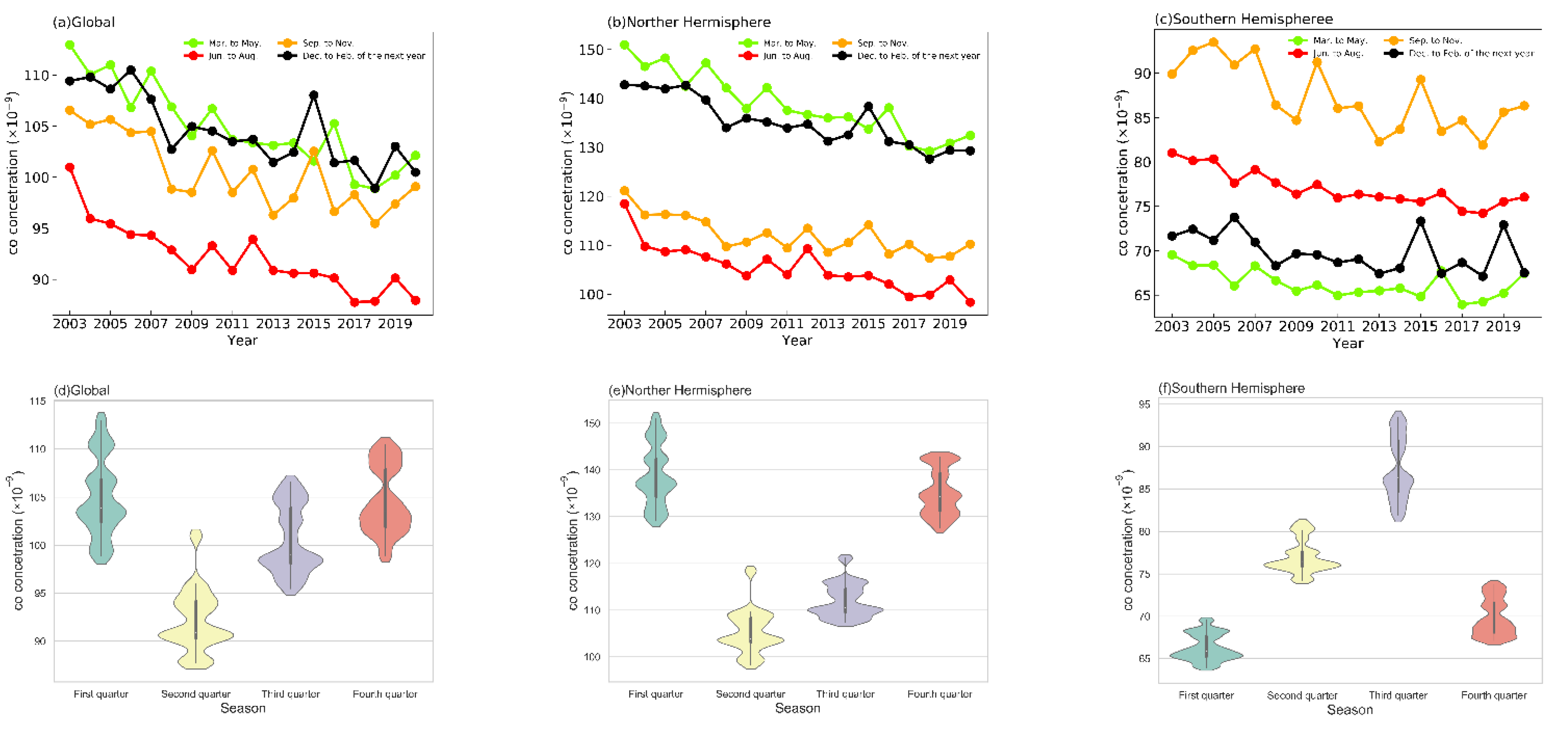
Since the four seasons in the southern hemisphere and the northern hemisphere are not the same, this section analyzes the global four seasons according to their quarterly distribution. The specific division is as follows: March to May stands for the first quarter; June to August stands for the second quarter; September to November stands for the third quarter; and December to February of the next year stands for the fourth quarter. Figure 4 shows the broken line chart and violin chart of the seasonal changes of the atmospheric pressure layer at 850 hPa in the world, and for the northern hemisphere and the southern hemisphere. Combined with the statistical analysis of the seasonal data in Table 1, it can be seen that the seasonal changes of CO in the world and the northern hemisphere are the same. It can be clearly seen from Figure 4a,d and Figure 4b,e that CO presents a “√” shape change during the four seasons of the year, which means CO concentration decreases from the first quarter and gradually increases after reaching the lowest value in the second quarter. It can be seen from Figure 4c,f that the CO concentration in the southern hemisphere shows a reverse change of “√” shape throughout the year, that is, the CO concentration increases from the first quarter and begins to decrease after reaching the peak in the third quarter; the reason may be that the seasonal variation of CO in the northern hemisphere accounts for a larger weight in the world due to the opposite seasons in the southern hemisphere and because of the majority of land in the northern hemisphere, as well as the more intensive plant growth and human activities, forming the same type of seasonal variation in the global and northern hemispheres, while the change type in the southern hemisphere is opposite. By observing the analysis in Figure 4a–c, it can be seen that CO concentration in the global and northern hemispheres show a downward trend, while that in the southern hemisphere shows a gentle change, which is the same as discussed in the previous discussion. According to Figure 4d–f and Table 1, under the influence of ground factors, the seasonal mean and variance of the northern hemisphere are significantly higher than those of the global and southern hemispheres, indicating that CO concentration in the northern hemisphere varies greatly and fluctuates violently. In addition, there are obvious discrete values of CO concentration during the first quarter in the global and northern hemispheres, while there are obvious discrete values in autumn in the southern hemispheres. From the perspective of probability distribution, the distribution of CO concentration during the four seasons in the global and northern hemispheres is extremely uneven, which may be influenced by regional factors and animal and plant activities.
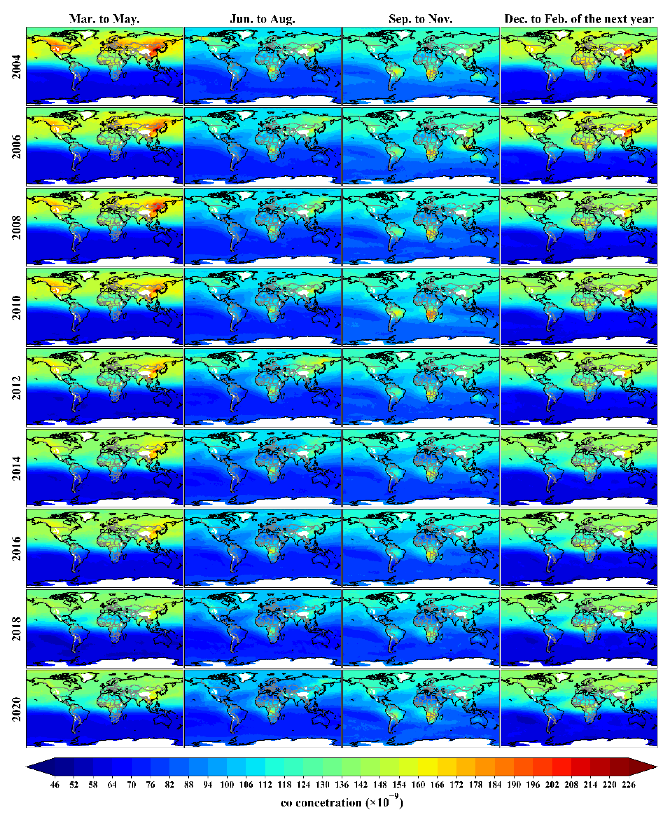
Figure 5 shows the spatial distribution of global CO concentration in the even number years of 850 hPa atmospheric pressure from 2003 to 2020. It is obvious from the figure that global CO concentration shows a decreasing trend, and the CO concentration in the northern hemisphere is higher than that in the southern hemisphere. As can be seen from the spatial distribution diagram of the four seasons, the CO concentration is highest during the first quarter in China in the northern hemisphere, and highest in the third quarter in southern Africa in the southern hemisphere. In addition, the CO concentration is high in some regions with rapid development and developed animal husbandry and heavy industry (such as East Asia, Africa, and North America). Especially in eastern China, high values of CO concentration often occur during the first quarter and fourth quarter, but default values occur in Greenland, Antarctica, and the Qinghai-Tibet Plateau. Due to the influence of altitude factors on the Qinghai-Tibet Plateau, the default value appears in the area of the Qinghai-Tibet Plateau. The specific reasons will be studied in East Asia in the following part. Antarctica and Greenland are relatively cold arctic climates where the temperature is low, the content of the vegetation is less, and human activity is relatively low, leading to low CO concentrations. In a year, the four seasons in Antarctica, Greenland, and the polar regions of the Qinghai-Tibet Plateau produce a low content of atmospheric pollution gases, such as CO.

4. Temporal and Spatial Distribution Characteristics of CO in East Asia

According to the analysis of the global CO temporal and spatial distribution map, it can be seen that the economic development in East Asia has been relatively rapid during the past 40 years, and human activities have been relatively intensive, resulting in high CO concentrations and violent fluctuations in this region. Therefore, this section mainly analyzes the spatial and temporal distribution characteristics of CO in East Asia. From the analysis of the space-time distribution characteristics of different pressure layers in the world, it can be concluded that the minimum and maximum values of different pressure layers in the troposphere are very different. Therefore, the minimum and maximum values of CO concentration in this layer are selected for the control of plotting the concentration range of different pressure layers in this section.

4.1. Spatial Variation Characteristics of CO at Different Pressure Layers in Troposphere

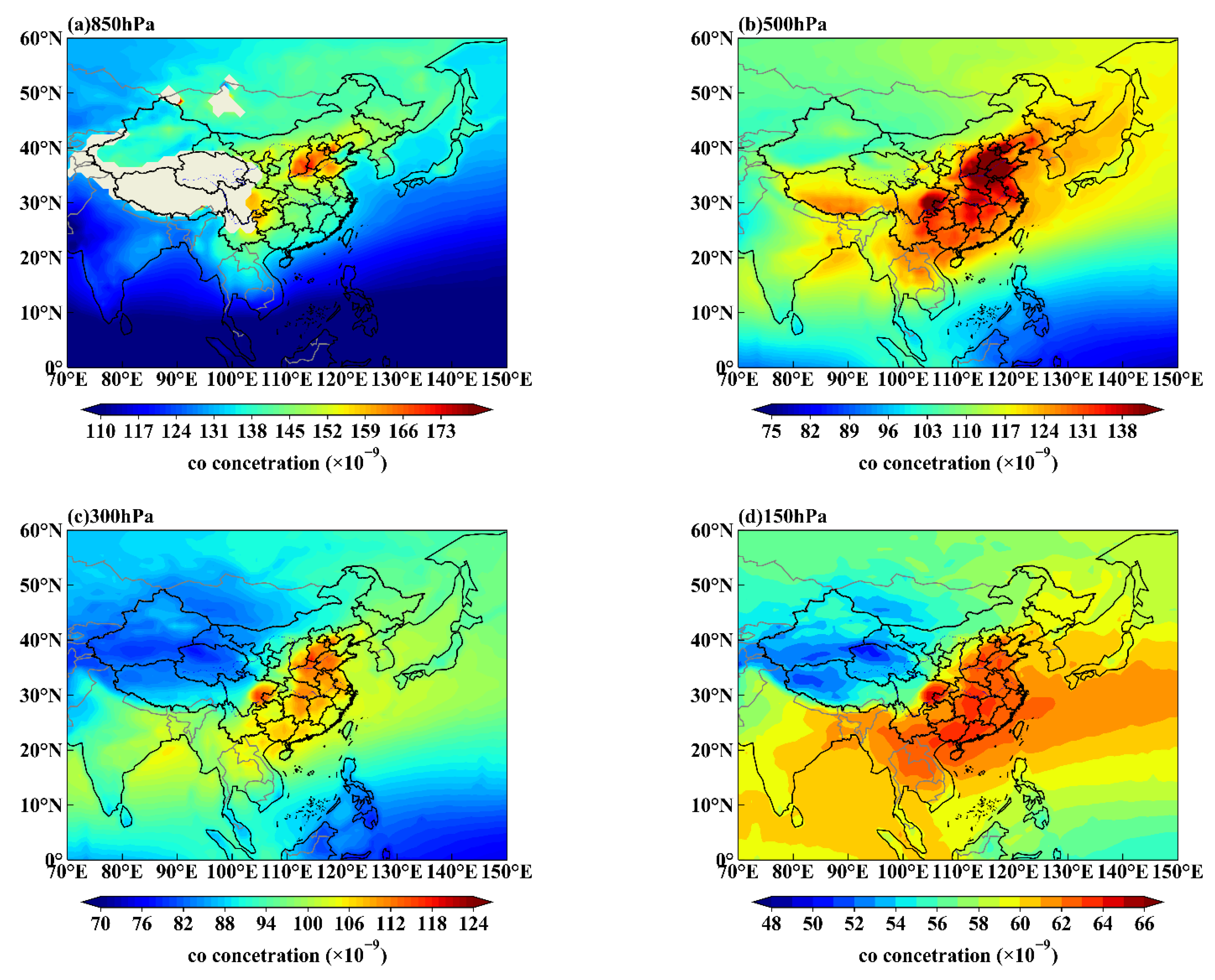
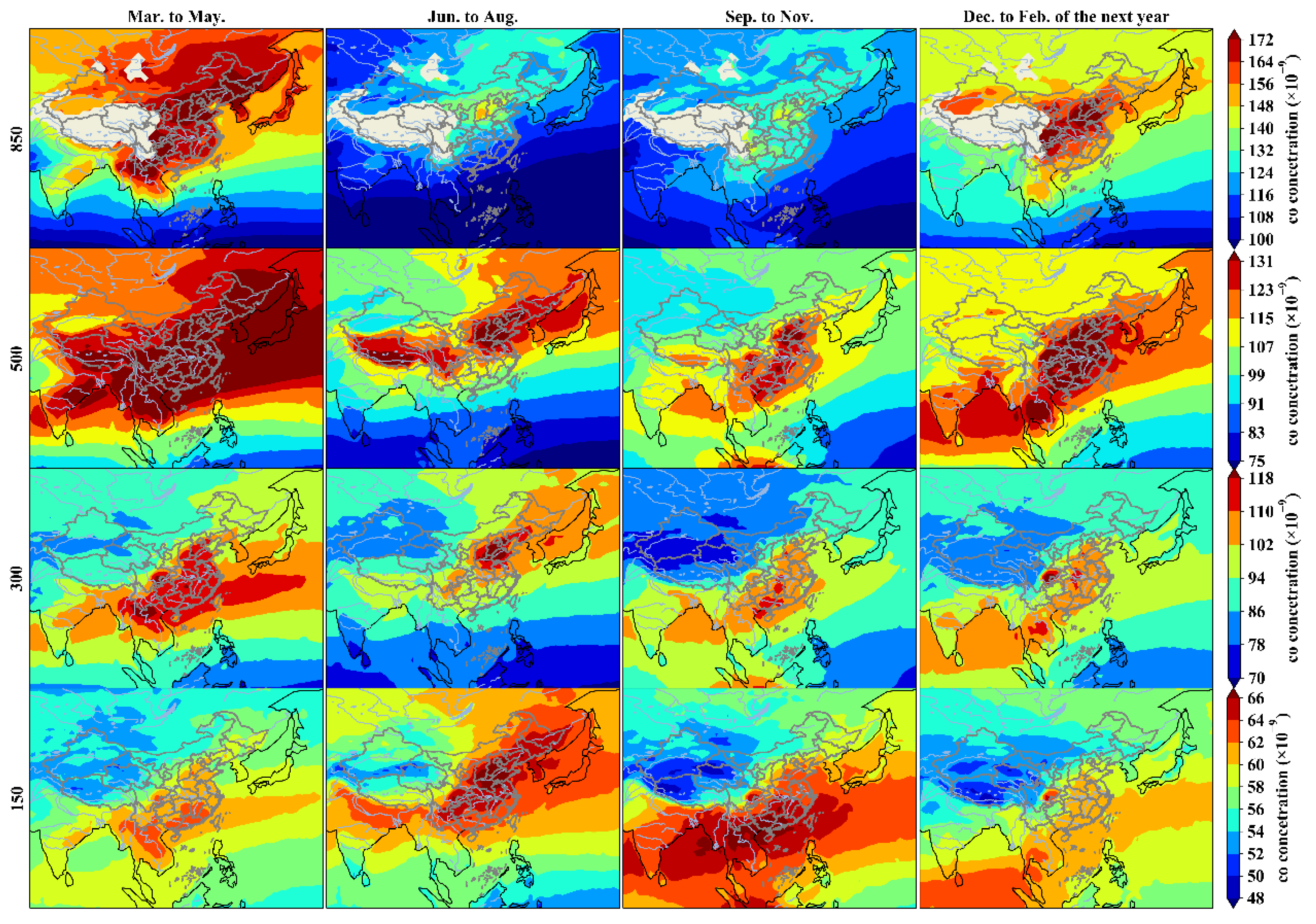
Figure 6 shows the spatial distribution of CO concentration in East Asia in the barometric layer at 850 hPa, 500 hPa, 300 hPa, and 150 hPa, respectively. Combined with the analysis of the mean, variance, and standard deviation of each barometric layer in Table 2, the average layer-by-layer concentration gradually decreases with the upward diffusion of the atmosphere and the horizontal movement of some aerosols, and the spatial distribution of each layer varies greatly—while the standard deviation of the four layers decreases gradually. The CO concentration becomes more and more stable with the increase in altitude.
Figure 6a shows the data for CO concentrations in the lower troposphere (850 hPa). It can be seen from the figure that most of the area in the Qinghai-Tibet Plateau is missing, because the average altitude of the Qinghai-Tibet Plateau is 1 km under 850 hPa atmospheric pressure, while the average altitude of the Qinghai-Tibet plateau is 4–5 km and the corresponding pressure is about 700 hPa to 500 hPa. Therefore, no specific study has been made on the 1000–700 hPa pressure layer in the Qinghai-Tibet Plateau. However, in East Asia, the data of longitude 110° E to the east is reliable. It can be seen that the CO concentration in some areas of eastern China (110° E~120° E, 35° N~40° N) is high, and the average total value of CO can reach 125.56 × 10⁻⁹—and the CO concentration in marine areas are significantly lower than that in land areas; this could be due to human activity and surface life. The CO high values in East Asia are mainly in the hinterland of central China (Beijing, Tianjin, and the neighboring provinces), Sichuan Basin, and Yangtze River Delta. Figure 6b shows the spatial distribution of CO at the middle troposphere (500 hPa). As can be seen from the figure, since the average altitude at 500 hPa is 5.5 km, there is no missing value of CO concentration in the Tibetan Plateau, which can better reflect the spatial distribution characteristics of CO in East Asia.
According to the analysis of the spatial distribution diagram in Figure 6, it can be concluded that between the pressure layers of 500 hPa and 150 hPa, the two main high-value areas in East Asia are the hinterlands of central China (Henan, Hebei, Shandong, etc.), the Sichuan Basin, and the southeast coastal area. In general, the spatial distribution of CO concentration in China is high in the east and low in the west. With the atmospheric pressure rising from 850 hPa to 150 hPa, the high-value area of CO concentration in China gradually shifts to the southeast coastal areas.

4.2. Temporal Variation Characteristics of Different Pressure Layers in Troposphere

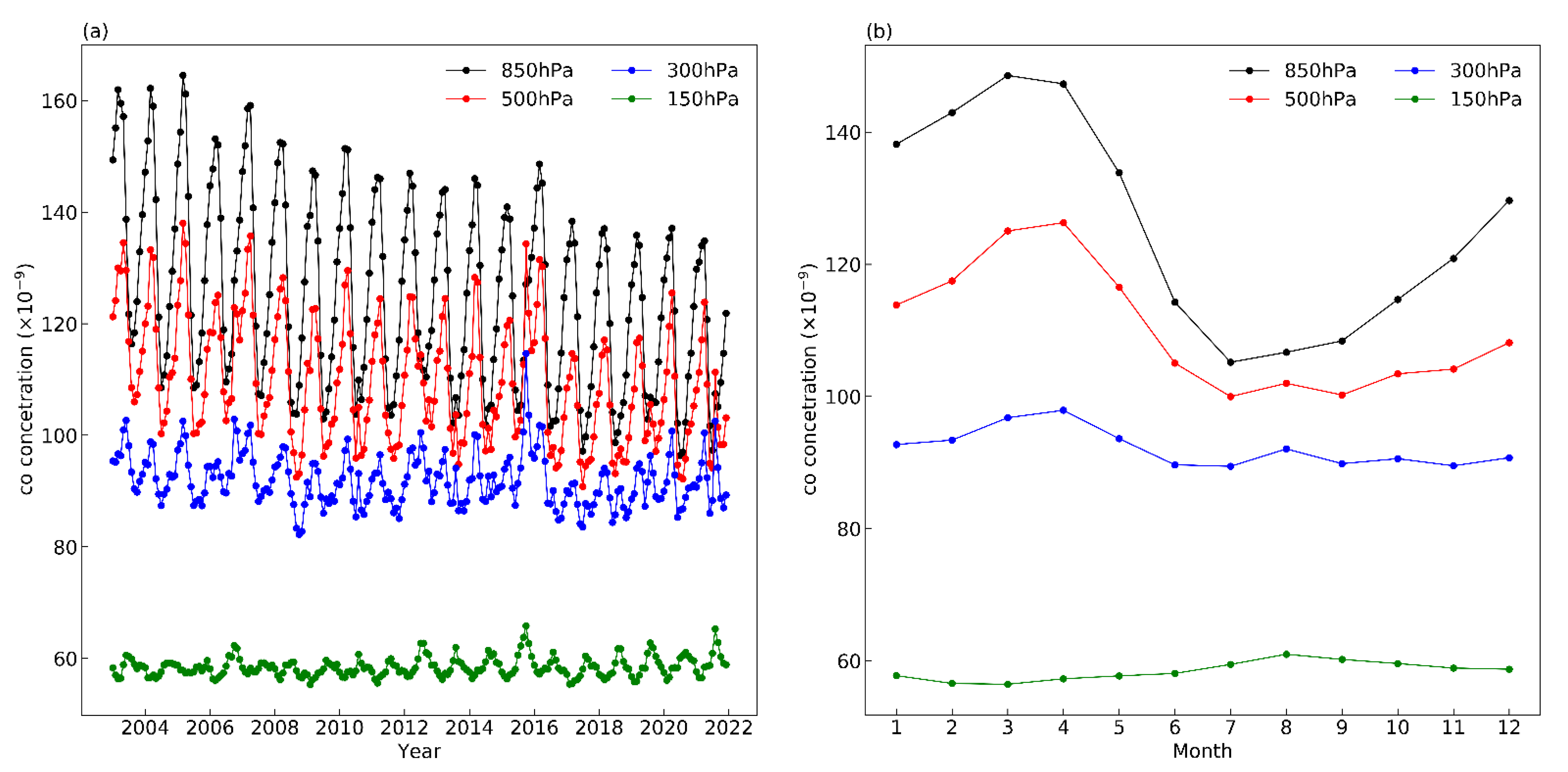
Figure 7 shows the time-series variation in the tropospheric CO concentration in East Asia.
It can be seen from Figure 7a that during the period from 2003 to 2020, when the atmospheric pressure layer is 850 hPa and 500 hPa, the CO concentration in East Asia gradually decreases periodically. As can be seen from the figure, the lower the troposphere is (that is, the closer it is to the ground), the more significant the change trend of CO concentration and the more severe the fluctuation is. Possible reasons for this are that CO is consumed by some OH free radicals in the atmosphere during upward transportation, which makes the concentration of CO more stable at high levels, and is affected by human factors due to its proximity to the ground (such as automobile exhaust emissions, fossil fuel combustion, and forest fire combustion, etc.). The CO concentration in the lower troposphere fluctuates greatly, while the CO concentration in the upper troposphere changes gently.
It can be seen from Figure 7b that monthly changes are obvious in the middle and lower troposphere (850 hPa and 500 hPa). At 850 hPa, CO increased gradually from January to March, reached the highest concentration in March, then decreased to the lowest value in July, then slowly increased again. At 500 hPa, CO concentration increased from January to April, reached the highest value in April, and then decreased to the lowest value in July, and then slowly increased.

4.3. Interannual Variation Characteristics of Different Atmospheric Pressure Layers in Troposphere

In order to analyze the annual change trend of CO concentration at different atmospheric pressure levels in East Asia, this section selected CO concentration data from 2003 to 2021 at different atmospheric pressure levels by year aggregation grouping. AIRS CO data can be divided into 24 atmospheric pressure layers. In this paper, 1000 hPa, 925 hPa, and 850 hPa are divided into lower troposphere, 700–400 hPa into middle troposphere, and 300–100 hPa into high troposphere. In this section, 850 hPa is selected as low troposphere, 500 hPa as middle troposphere, and 300 hPa as high troposphere CO data. Then, the CO concentration of different pressure layers was linearly fitted.
Combined with Figure 8 and Table 3, it can be observed that: In the lower troposphere, as shown in Figure 8a, the average CO concentration in East Asia was significantly higher than the global average CO concentration during the same period. On the whole, the CO concentration in both the world and East Asia showed a significant downward trend. The interannual linear regression between the world and East Asia revealed that the correlation coefficients were −0.904 and −0.954. The fitting slopes of CO concentration in the lower troposphere of the world and East Asia are −0.552 × 10⁻⁹ and −1.129 × 10⁻⁹, respectively. In other words, CO concentration decreased by 5.52 × 10⁻⁹ and 11.29 × 10⁻⁹ per decade in the global and East Asia regions, respectively. The average annual decline rate of CO concentration in East Asia was larger than that of the global rate during the same period. It can be seen from Figure 8b that the variation trend of CO concentration in the middle troposphere and in East Asia is similar to that in the lower troposphere, showing a downward trend, but the trend is gentler than that in the lower troposphere. After the annual average linear regression for the global and East Asian regions, they both pass the significance test of 0.01, and the Pearson’s correlation coefficients of the two are −0.662 and −0.825 respectively, which are significantly negatively correlated with the annual growth. The fitting slopes of global and East Asian CO concentrations in the middle troposphere are −0.297 × 10⁻⁹ and −0.700 × 10⁻⁹, respectively, that is, the concentration of CO in the world and East Asia decreases by 2.97 per 10 years ×10−9 and 7.00 × 10⁻⁹, respectively, and the global decline rate ratio is still smaller than that in East Asia. Figure 8c shows that the change trend of global and East Asian CO concentration in the upper troposphere is very different from that in the middle and lower troposphere. First, the change in CO in the upper troposphere is relatively gentle, and there is no obvious upward and downward trend. After linear fitting, it is found that the correlation coefficients of the two are −0.037 and −0.417, and neither of them has passed the significance test of 0.01, indicating that in the upper troposphere, although the regional and global CO concentration in East Asia is negatively correlated with the year, the change trend is not obvious.

4.4. Interannual Variation in Different Latitudes of Different Tropospheric Pressure Layers

In order to further study the variation of CO concentration in different latitudes in East Asia under different pressure layers, this paper analyzes different latitudes according to the division of seasonal years (September 2002–August 2003 is the average CO concentration in different latitudes in 2002) from September 2002 to September 2021. The longitude and latitude range of East Asia is: latitude; 0° N~60° N, longitude; 70° E~150° E. Figure 9a shows the interannual variation diagram of different latitudes at 850 hPa in the barometric layer. From the vertical view of the figure, the concentration in the latitude zone from 0–10° N to 20–30° N rises section by section. After 20–30° N, the change of CO concentration is not obvious, showing a state of line adhesion. From the horizontal (interannual change) of each latitude segment in the figure, each latitude segment shows a gradually decreasing trend at 850 hPa, which is consistent with the interannual change trend of the whole East Asia region studied above. Figure 9b–d show the interannual variation of CO at 500 hPa, 300 hPa, and 150 hpa, respectively. From the figure, it can be seen that with the gradual increase of the pressure layer, the interannual variation of CO concentration at each latitude is more disordered, which may be due to the different absorption capacities of aerosols at different latitudes when CO diffuses to the upper layer, resulting in more and more disordered CO concentration at different latitudes of different pressure layers. As can be seen from the figure, in the interannual variation of CO at different atmospheric pressure layers and at different latitudes, the concentration of CO suddenly increased in 2015, especially at low latitudes. According to the data consulted, it was found that fires occurred in East Asia many times in 2015. For example, an explosion of industrial alcohol in Kunming, Yunnan Province; a major fire and explosion accident in Tianjin, an explosion of a chemical plant in Shandong Province, and a fire accident in Harbin, etc., may all be the cause of the sharp increase in CO concentration. In addition, the change of CO concentration may also be related to atmospheric temperature. According to the 2015 Climate Status Statement released by the World Meteorological Organization, due to the influence of human activities and strong El Niño, May 2015 be the hottest year in the world, and the ocean temperature will increase significantly and the ocean heat will break the record again. The mutation of CO concentration was most obvious in the low latitude region of East Asia, where the proportion of low latitude ocean region was larger.

4.5. Seasonal Spatial Variations of Different Atmospheric Pressure Layers in Troposphere over the Years

In order to further analyze the seasonal spatial variation of CO in East Asia, the AIRS satellite sounder was used to obtain the seasonal variation of CO concentration in different atmospheric pressure layers from September 2002 to August 2021. Since East Asia is located in the northern hemisphere, spring, summer, autumn, and winter were divided according to the seasonal and monthly variations of the northern hemisphere. The spring in East Asia is from March to May, the summer is from June to August, autumn is from September to November, and winter is from December to February. Figure 10 shows the spatial changes in East Asia during four seasons at 850 hPa, 500 hPa, 300 hPa, and 150 hPa from 2002 to 2020.
As can be seen from the strip of each layer in the figure, the CO concentration gradually decreases with the increase in the altitude layer, which is consistent with the previous conclusion. From space, the four seasons change each layer of CO concentration that exists because of obvious seasonal change at 850 hPa due to high altitude areas, such as the Qinghai-Tibet Plateau satellite, which did not detect the CO concentration, so the default value of the obvious—the spring and winter CO concentration—were significantly higher than that of summer and autumn, and the high-value area in the middle and lower reaches of the Yangtze River in China, as well as the central plains and coastal regions in northeast China. The possible reason for this is that in winter and spring, when the weather is cold and heating is supplied in northeast China, a large number of fossil fuels (coal, oil, natural gas, etc.) will be burned, resulting in a large number of polluting gases, such as CO. The development of heavy industry in the hinterlands of central China and coastal areas (for example, iron and steel smelting, machinery industry, and chemical industry, etc.) will produce harmful gases, such as methane and CO, and greenhouse cultivation in recent years gradually increased due to this because of the need to increase greenhouse temperature in winter, given that most people will use a coal fire for heating. Given that incomplete combustion in the process also produces CO, this may be one of the causes of CO in the spring and winter; secondly, this may be due to the festival in the spring and winter when temperatures are low, which results in the diffusion of some discrete gases and pollutants into the air. However, in the summer, due to rising temperatures, the diffusion of atmospheric pollutants is accelerated, and the chemical reaction is active in the atmosphere in the summer, making it easier for CO oxidation and OH particles to produce carbon dioxide—resulting in the CO concentration being low in the summer. In addition, there is more rain in autumn because the rain also plays a role in washing and cleaning some pollutants in the atmosphere, which may also cause the low concentration of CO in autumn. The seasonal spatial variation varies greatly from 500 hPa to 850 hPa. Although the CO concentration is still high in spring and winter, the coverage area of the high-value area increases gradually, and the value is also detected in areas with higher elevations (such as the Qinghai-Tibet Plateau), especially in spring, where the high-value areas of CO concentration almost cover the whole region of China. At 300 hPa and 150 hPa atmospheric pressure layers, the spatial distribution of CO in the upper troposphere is quite different from that in the middle and lower troposphere. In the upper troposphere, the CO concentration is higher in the southeast and lower in the northeast in spring, autumn, and winter, and the high-value areas are always located in the southeast coastal region. In summer, the CO concentration in the northeast and central China is significantly higher than that in the south. This may have to do with the temperature of the atmosphere as the gas spreads upward and because of the seasonal wind directions.

5. Analysis of Temporal and Spatial Variation Trend of CO

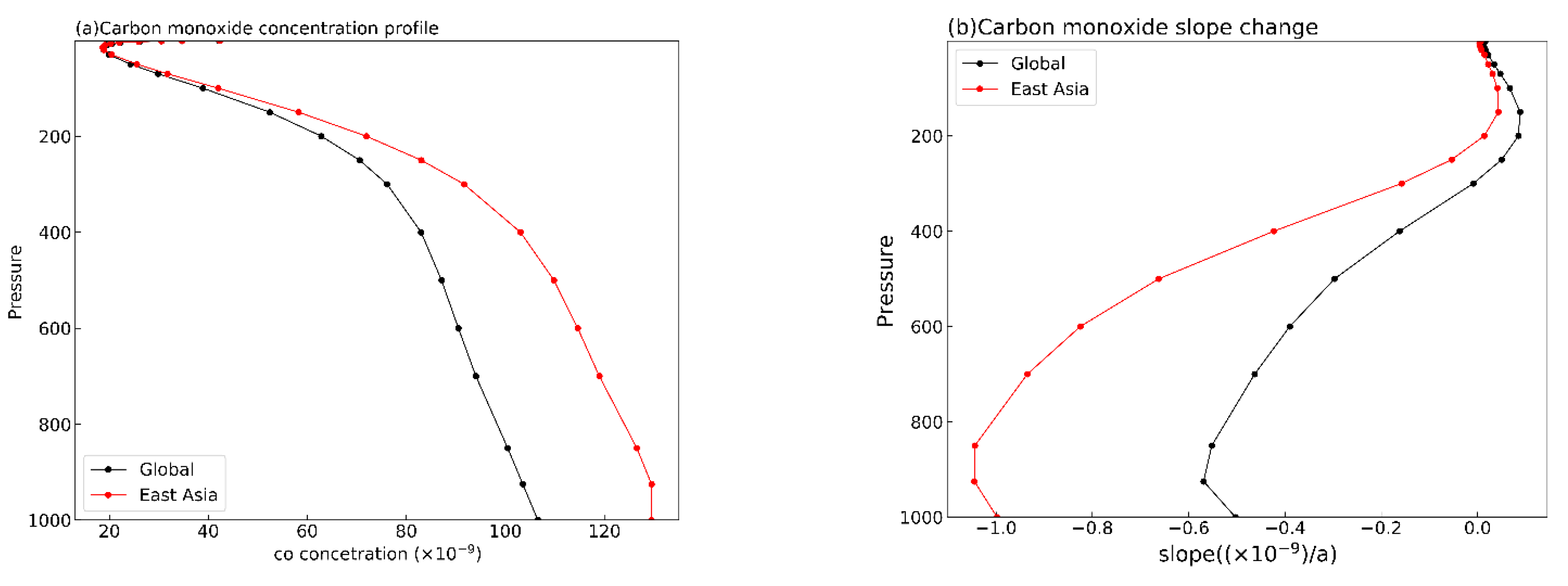
In order to explore the variation trend of tropospheric CO concentration in the world and East Asia deeply, based on CO concentration data from 2003 to 2021, this section uses the MK trend test and EOF method to analyze the spatiotemporal variation of global CO concentration. Figure 11 shows the annual mean value and change rate of CO concentration at 24 vertical layers in the world and East Asia from 2003 to 2021. It can be seen that the CO concentration and decline rate in the troposphere in East Asia are always higher than those in the world, and the mean value and change rate of CO concentration gradually fits with the increase of altitude. When the atmospheric pressure reached the stratosphere, the line chart of CO concentration and change rate in the global and East Asia regions gradually coincided. The analysis showed that the change of CO concentration in the troposphere was relatively complicated. Given that the CO concentration in the polar regions in the lower troposphere (Greenland, Qinghai-Tibet Plateau, and Antarctica, etc.) was affected by geographical factors, it was difficult to detect the CO concentration. The middle and upper troposphere was selected for analysis of the temporal and spatial variation trend of the CO concentration.

5.1. Analysis of Long-Term MK Space Variation Trend of CO Concentration in the Global Middle and Upper Troposphere for many Years

In order to better predict the change trend of global CO concentration, the MK trend test and prediction method are used in this section to predict the advance trend test and Sen slope estimation of each fence grid point in the global middle and upper troposphere (500 hPa, 300 hPa, and 100 hPa) from 2003 to 2021, as shown in Figure 12. Figure 12a,b shows the MK z-value trend test and Sen slope space estimation prediction diagram when the atmospheric pressure layer is in the middle troposphere (500 hPa), respectively. It can be seen from the figure that CO concentration shows a downward trend in more than 90% of the global regions, and the decreasing rate in the northern hemisphere is significantly higher than that in the southern hemisphere, and the CO concentration drops especially rapidly in East Asia. In particular, the decline rate is the largest in the Central Plains and southeast regions of China, which may be related to the promulgation of low-carbon development and the increase of vegetation planting in China in recent years—so that the CO emissions in land areas gradually decreased, and the decline rate is relatively fast compared with other regions. Figure 12c,d and Figure 12e,f show the spatial trend variation of the upper troposphere (300 hPa and 100 hPa). The figure shows that with the rise of the altitude level, the spatial trend of CO changes greatly. At 300 hPa, there are many high values of the CO concentration rising trend between 30° S and 30° N, but there is still a significant downward trend of CO concentration in most parts of East Asia. When the pressure layer reaches 150 hPa, there is an obvious high-value belt of CO rising from the south latitude to equator. At this time, there was an obvious upward trend in most parts of the northern hemisphere, but there was still an obvious downward trend in Antarctica, Greenland, and some parts of East Asia (Beijing, Tianjin, Hebei, Shandong, and Sichuan in China).
At different altitudes, there is a huge difference in the spatial variation trend of CO, which may be mainly due to the reduction and oxidation of CO, which is prone to chemical reactions. In the upward diffusion of CO with atmospheric circulation, under different latitudes, humidity and temperature, and other spatial factors—under certain conditions—CO easily reacts with OH, O, H, and other free particles in the air. Due to the complex atmosphere of the troposphere, there are huge differences in the variation trend of CO in different regions at different altitudes.

5.2. Analysis of Temporal and Spatial Modal Characteristics of Global Tropospheric CO Concentration over the Years

In this section, the monthly average data of global atmospheric CO concentration are processed by using the detection data from 2003 to 2021 to obtain the annual average CO concentration of different atmospheric pressure layers in the troposphere. In this section, 100 hPa, 500 hPa, and 850 hPa are selected to represent the variation trend of CO in the high and low troposphere, respectively. Then, the EOF method (empirical orthogonal function analysis method) was used for modal decomposition, and the variance contribution rates of the first six modes of CO concentration in the three global atmospheric pressure layers were obtained, as shown in Table 4. The larger the variance contribution rate was, the more it could reflect the spatial and temporal distribution characteristics of atmospheric CO concentration in different atmospheric pressure layers in the global troposphere over 19 years.
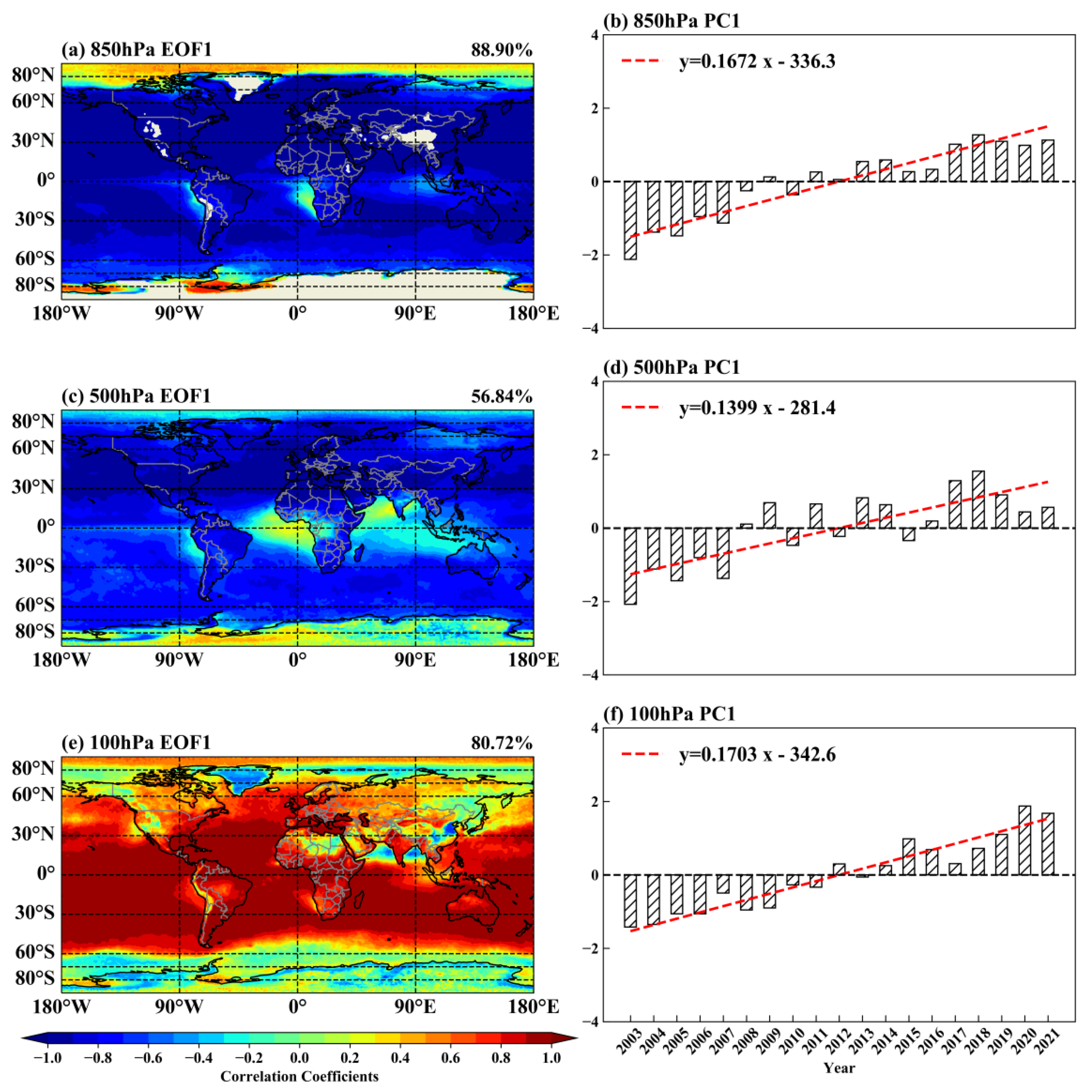
It can be seen from Table 4 that the three levels of the troposphere before the six modal cumulative variance contribution rates were over 93.13% because each layer—EOF1, which accounted for the largest area—has can basically reflect the characteristics of the spatial and temporal variations of different pressure layers, so this section is mainly used for different air layers of the first mode of the corresponding coefficient of space and time change. Figure 13 shows the spatial distribution and time coefficient of the pressure layer in the first mode of 850 hPa, 500 hPa, and 100 hPa.
Figure 13a,b show the spatial distribution of EOF1 and the time coefficient of PC1 when the pressure layer is in the lower troposphere (850 hPa), respectively. As can be seen from the spatial distribution diagram in Figure 13a, except for positive values in a few areas such as Antarctica and default values in some polar regions, negative values are observed in other regions of the world. This indicates that the global spatial variation trend in the lower troposphere is consistent from 2003 to 2021, that is, the CO concentration in the lower troposphere increases or decreases simultaneously. Combined with the time coefficient figure in Figure 13b, it can be seen that the time coefficient was negative from 2003 to 2008, but positive after 2011, indicating that the global atmospheric CO concentration in the lower troposphere showed a downward trend. Especially after 2017, the time coefficient value was very large and positive. This reflects that the global CO decline trend after 2017 is extremely significant.
Figure 13c,d show the spatial distribution of EOF1 and the time coefficient of PC1 in the middle troposphere (500 hPa), respectively. It can be seen from the spatial distribution diagram of Figure 13c that the spatial variation trend of the middle troposphere and lower troposphere is roughly the same. Except for Antarctica, the Arabian Sea, and the Bay of Bengal, other regions of the world show negative values. Combined with the time coefficient diagram of Figure 13d, it can be seen that the time coefficient was negative during 2003–2007. The positive values are mostly from 2008 to 2021, which indicates that the global atmospheric CO concentration in the middle troposphere has a declining trend during the past 19 years, which is consistent with the spatiotemporal variation trend of the global atmospheric CO concentration in the middle troposphere analyzed by MK above.
Figure 13e,f shows the spatial distribution of EOF1 and the time coefficient of PC1 when the pressure layer is in the upper troposphere (100 hPa), respectively. As can be seen from the spatial distribution diagram in Figure 13e, the spatial variation trends of the upper troposphere and the middle and lower troposphere are very different, with negative values in Greenland, the Mengjiala Bay Sea, South China Sea and parts of Sichuan, and North and East China, while there are positive values in other parts of the world. Combined with Figure 13f’s time coefficient figures, it can be seen that the time factor in the 2003–2011 annual average is negative, while later in 2012, when it is in the majority, it is positive. The CO concentration in the upper troposphere in 2012 in many parts of the world is increasing, but the South China Sea in China, as well as Sichuan, Beijing, Tianjin, Hebei, and Shandong, among other places, are part of a downward trend. This is consistent with the previous analysis of the spatiotemporal variation trend of global atmospheric CO concentration in the upper troposphere for 19 years by MK.

5.3. Prediction and Analysis of Near-Surface Global and East Asian CO Concentration Using the Three-Exponential Smoothing Model

In this section, the atmospheric pressure layer is selected as 850 hPa to conduct a time-series data prediction and analysis on the monthly mean concentration of CO in the global and East Asian regions for the 19 years from January 2003 to December 2021. As can be seen from the above analysis, CO concentration in the near-surface region (850 hPa) in the global and East Asian regions shows a periodic trend change. Therefore, this section carries out a prediction and analysis by constructing a three-exponential smoothing model that is suitable for seasonal changes.
Figure 14 shows the prediction of CO concentration in the global and East Asian near-surface regions using the three-exponential smoothing model with a 95% confidence interval. It can be seen from Figure 14 that the three-exponential smoothing prediction model has a good prediction effect on the global and East Asian regions, and the errors between the predicted value and the real value are small—all within the 95% confidence interval. As can be seen from the prediction results, the near-surface CO concentration in the global and East Asian regions will continue to maintain a seasonal downward trend in the future. Table 5 is the evaluation index of the model. It can be seen from the model index that the MAE and RMSE of the three-exponential smoothing prediction model in the world and East Asia are relatively low, while the is relatively high—both above 0.9—and the prediction accuracy is relatively high. Therefore, the model is relatively reliable for the future global and East Asian CO concentration temporal variation trend.

5.4. Construction of Global CO Concentration Prediction Model Based on VMD-LSTM

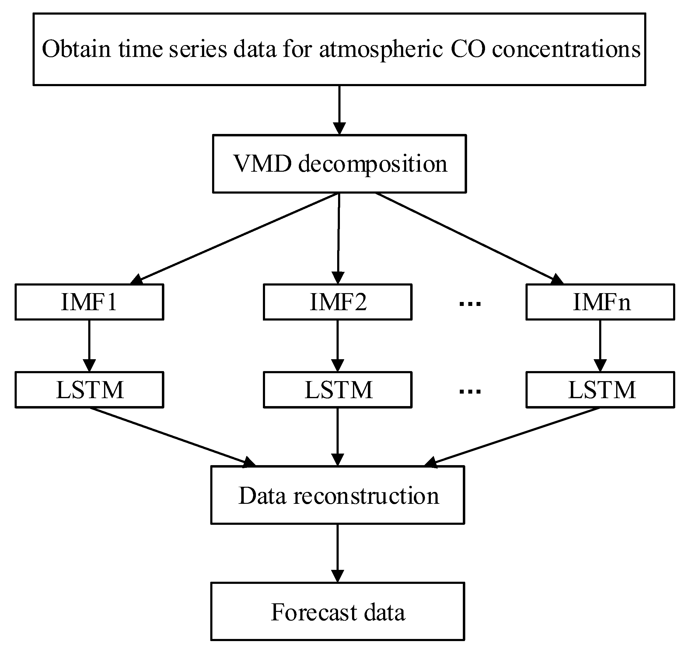
In recent years, with the rapid development of deep learning, artificial intelligence based on deep neural networks has been widely used in various fields. Among them, LSTM is a special time recursive neural network. Due to the non-linearity and non-stationarity of atmospheric CO concentration time-series data, the prediction accuracy of using an LSTM model alone is not ideal. Therefore, in this section, VMD is used to preprocess the CO time-series data, extract the essential features in the complex series, and then LSTM is used for the prediction and reconstruction, respectively. Finally, the evaluation index is used to evaluate the model, and the evaluation accuracy of the prediction is compared with that of the three-exponential smoothing model. In Figure 15, the framework diagram of the VMD-LSTM atmospheric CO concentration prediction model is shown.
First, the experimental data used in this section are the 228-month average CO concentration data in the troposphere for 850 hPa for the global region from January 2003 to December 2021, with a time resolution of months. Secondly, the dataset is divided. In this section, the CO concentration time-series dataset is divided into a training set and a verification set according to the ratio of 8:2. The prediction model is generated using the training set. Finally, the error and accuracy of the model are tested using the verification set data.
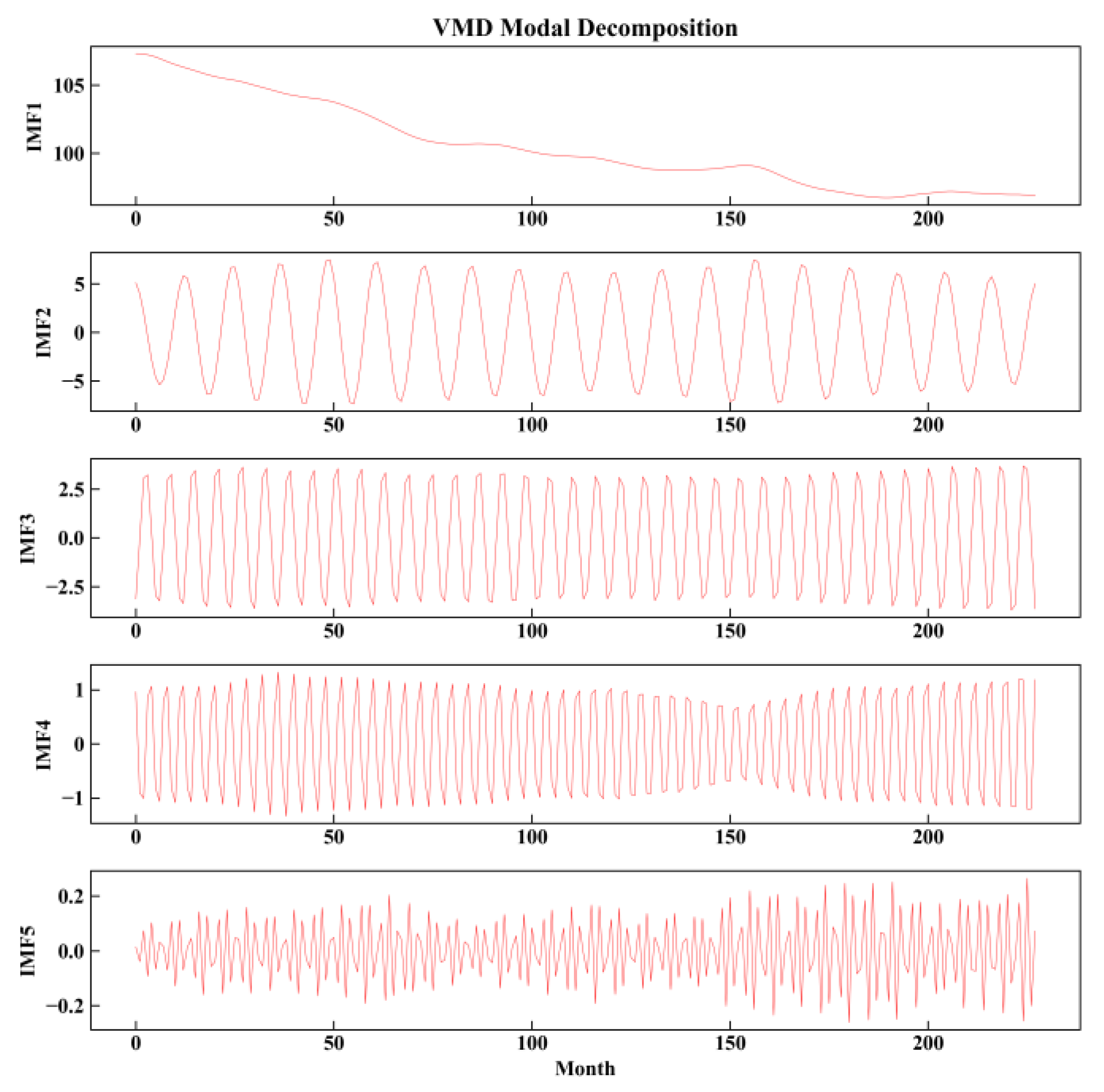
In Figure 16, the decomposition diagram of the CO concentration VMD signal is shown. VMD confirms the appropriate number of variational modes according to the distribution of the central frequency. The decomposition effect of VMD is mainly affected by the value of the number of modes. For example, when the number of modes is small, some important information from the original data may be filtered out, thereby affecting the prediction accuracy. If the number of modes is large, it may cause mode repetition or noise. After many experiments in this paper, it was concluded that it is optimal when the number of modes is 5, that is, the original data is decomposed into 5 IMF. The bandwidth alpha is 7000, the noise tolerance tau is 0, and the control error constant Tol is 1 × 10⁻⁷. The model decomposes the 228-month CO concentration time-series set. The IMF components are ranked from low frequency to high frequency. Imf1 fluctuates greatly, representing that the overall change trend of CO concentration is similar to the residual component of EMD decomposition and shows a downward trend. Imf2, imf3, and imf4 have good periodic waves and strong regularity. The side reaction CO concentration shows a periodic change trend, which is consistent with the conclusion drawn from the previous analysis of the global monthly average change trend of CO.
Based on the VMD decomposition data, each IMF is predicted by LSTM, as shown in Figure 17. There is a comparison between the real value and the predicted value of the training set and the verification set of the VMD-LSTM prediction model. It can be seen from Figure 17 that the VMD-LSTM prediction model has a good fitting effect and a high degree of agreement on both the training set and the verification set. The comparative analysis of the three-exponential smoothing model and VMD-LSTM by using the evaluation index shows that the Mae and RMSE of VMD-LSTM are lower than those of the three-exponential smoothing model, which proves that the prediction effect of the VMD-LSTM mixed model is better.

6. Discussion

6.1. Temporal and Spatial Changes and Trends of Atmospheric CO Concentration in the World and East Asia

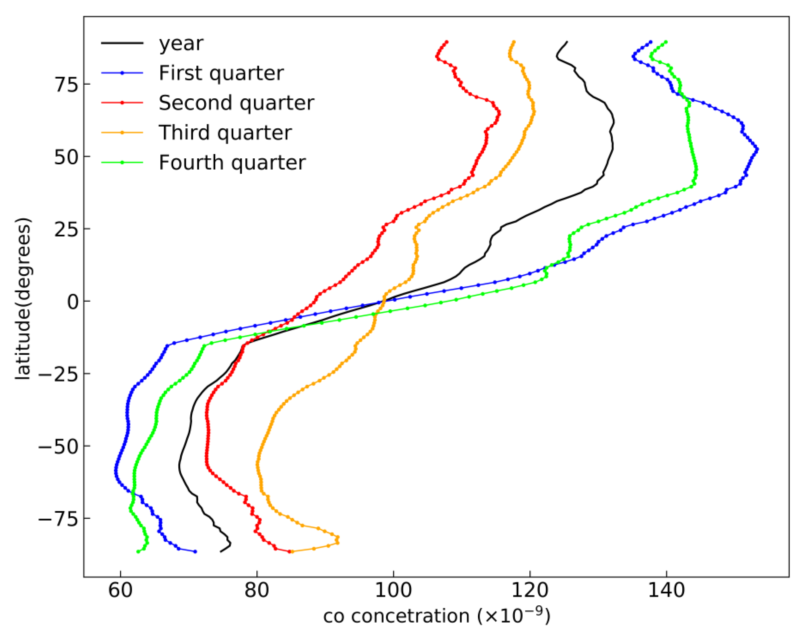
Previous scholars’ research on the temporal and spatial distribution of global CO shows that the atmospheric CO content in the northern hemisphere. is higher than that in the southern hemisphere, and it changes periodically. The highest season of the northern hemisphere is the first quarter, while the highest season of the southern hemisphere is the third quarter [12,13,14], which is consistent with the conclusion of this paper in analyzing the temporal and spatial variation characteristics of global near-surface CO (Figure 3 and Figure 4). In order to further highlight the change of CO concentration near the ground in the northern and southern hemispheres, this section uses the CO concentration data when the pressure layer is 850 hPa to draw the contribution analysis diagram of the global four seasons to the annual zonal average concentration of CO, as shown in Figure 18. It is obvious from the figure that in the south of the equator, the contribution of the second quarter and third quarter festivals to the annual CO concentration is significantly higher than that of the first quarter and fourth quarter. As well, the third quarter contributes the most to the annual CO concentration, while in the north of the equator, the first quarter and fourth quarter have a higher contribution to the annual CO concentration. In the fourth quarter, it can be seen from the interannual gradient change that the latitude shows a slow downward and upward trend from 90° S to 55° S, and a slow upward trend from 55° S to 15° S. Given that the CO concentration in the northern hemisphere is higher than that in the southern hemisphere, the change speed will increase when the southern hemisphere transits to the northern hemisphere, that is, 15° S–10° N shows a fast upward trend when 10° N starts to show a slow upward trend, and when the latitude is around 50° N, it will reach the maximum—and then the high latitude area will show a slow downward trend.
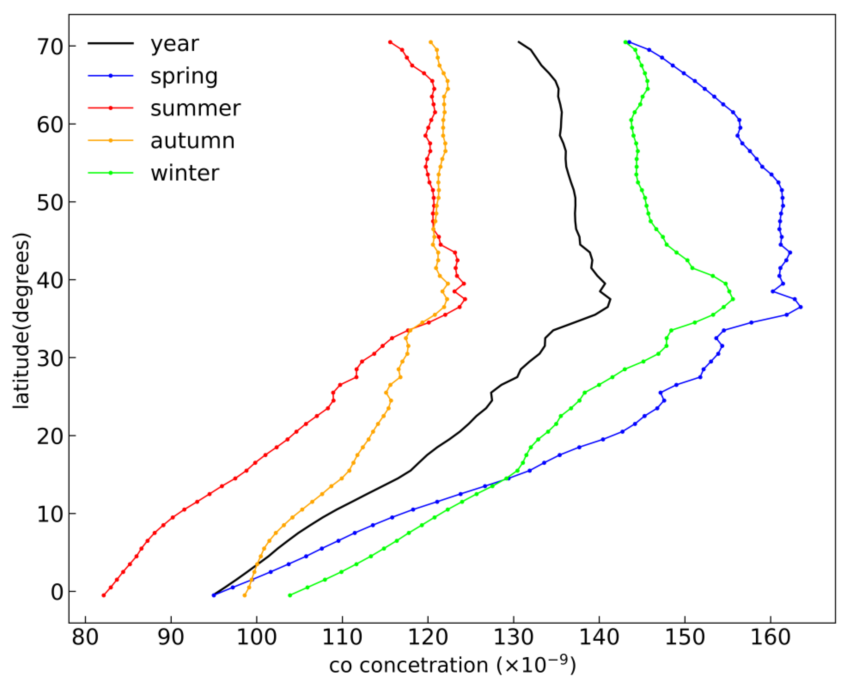
Some scholars have found that some regions with dense traffic, frequent industrial activities, and a large population base (such as East Asia, India, and North America) are regions with high total CO column values [34,35], which is consistent with the conclusions of this paper on the spatial distribution of CO concentration in different atmospheric layers in the troposphere (Figure 2). Zhang X et al. [36] studied the total amount of CO column in Asia in the four seasons. It was concluded that the total amount of atmospheric CO column in spring and winter in Asia is higher than that in summer and autumn, which is consistent with the trend described in this paper for the four season spatial variation of CO concentration in different troposphere layers in East Asia from 2003 to 2020. In order to further explore the four season variation trend of the near-surface CO concentration in East Asia, in this section, the atmospheric pressure layer is used to draw the contribution analysis diagram of the four seasons in East Asia to the annual zonal average concentration of CO (Figure 19) for the 850 hPa CO concentration dataset. From the diagram, it can be concluded that the contribution of spring and winter to the annual CO concentration is significantly higher than that of summer and autumn.
Zhang X et al. [36] used MOPITT and AIRS sounding instruments to study the total amount of CO column from 2003 to 2017, and found that there was a strong interannual change in Asia. In other words, CO reached its peak in 2015 due to large-scale fire events (the year of El Niño) possibly caused by drought conditions [37,38], which is consistent with the conclusion obtained in this paper on the interannual variation of different atmospheric pressure layers at different latitudes in East Asia. Zhang X et al. [36] and Worden H M et al. [16] found that the measured values of the general column of CO in the northern hemisphere showed a significant decreasing trend, and the decreasing trend was most obvious in eastern China, which was consistent with the conclusion of this paper on the trend change of CO concentration in different atmospheric pressure layers in the global troposphere. Although in the past most scholars studied the time and space distribution of CO, the important factor is the total global column analysis—which is not for the rapid development of global and regional CO concentration stratification research—though this paper mainly deals with the rapid development of global and regional tropospheric CO concentration in East Asia through a modal analysis and prediction research of time and space.

6.2. Discussion and Analysis on Influencing Factors of Tropospheric Atmospheric CO Concentration

In the past, many scholars found that the change of atmospheric CO concentration was mainly caused by the natural environment and human activities, such as Yin Y et al. [39]. This is mainly due to the improvement of China’s industrial combustion efficiency in recent years and the reduction of emissions of polluting gases. Zheng B et al. [23] used a MOPITT detector to invert the CO data and found that the CO concentration generally decreased in East Asia from 2005 to 2006, which is consistent with the conclusion reached in the analysis of the temporal and interannual changes in East Asia from 2003 to 2020 in this paper (Figure 7 and Figure 8). The decreasing trend of CO in East Asia is mainly caused by the gradual reduction of China’s resources. According to MEIC data, it is estimated that the main four units of CO emission reduction are the iron and steel industry, residential sources, automobile combustion, and the construction industry. Some scholars believe that the change of atmospheric CO concentration may be caused by fire and biological combustion in the natural environment. Some scholars find that the peak value of CO concentration is usually consistent with the number of fires occurring in the region or the world in the same year. Zhang X et al. [36] studied the total amount of CO columns in fire-prone regions of Asia (southern Siberia, Indochina Peninsula, and Indonesia) and found that biocombustion had a great influence on CO concentration in the region, especially in fire-prone seasons.
The above studies indicate that ground factors have a great impact on CO emissions, but CO entering the atmosphere mainly reacts with OH, so the concentration of OH in the atmosphere directly affects the trend of CO concentration. As the OH concentration is affected by various atmospheric components such as solar radiation, water vapor, methane, and so on, the water vapor, methane concentration, and atmospheric temperature indirectly affect the change of CO concentration. IA Girach et al. [40] used MOPITT data to study these effects and found that the increase in tropospheric water vapor is part of the reason for the decline of total CO column. Due to the low water vapor content and gas concentration in the middle and upper troposphere, this section conducts a correlation analysis between the CO concentration and atmospheric temperature, methane, and water vapor in the lower troposphere. Table 6 shows the correlation between the global atmospheric temperature, methane, water vapor, and CO in the lower troposphere (1000 hPa, 925 hPa, and 850 hPa) from 2003 to 2021.
It can be seen from Table 6 that in the lower troposphere, CO is negatively correlated with atmospheric temperature, methane concentration, and water vapor content, all of which pass the significance test of 0.01. The reason is that CH4 reacts with OH in the atmosphere to further reduce the concentration of OH, thus indirectly increasing the concentration of CO. Although CO is difficult to dissolve in water, under certain environmental conditions, CO can dissolve in water vapor, and the OH concentration can also come from water vapor at a certain temperature, further increasing the concentration of OH so as to reduce the concentration of CO in the atmosphere. It can be concluded that the rise in methane, water vapor, and atmospheric temperature in the troposphere is partly responsible for the reduction of CO concentration. As methane and water vapor are both greenhouse gases, when greenhouse gases increase in the lower troposphere, which is relatively low from the ground, they will lead to a strong greenhouse effect in some areas. The rise of greenhouse gases and atmospheric temperature will not only accelerate the pace of global warming but also affect the precipitation change in some areas.

7. Conclusions

In this paper, the spatial–temporal modal analysis and prediction of CO concentration in the troposphere of the world and East Asia from 2002 to 2021 were studied by using AIRS data inversion with high accuracy and long time-series. The effects of temperature, methane, and water vapor on CO concentration in the troposphere are also discussed. The following conclusions are drawn:
The spatial distribution of CO varies greatly under different pressure layers, and the CO concentration in the northern hemisphere is higher than that in the southern hemisphere as a whole. The CO concentration in the upper troposphere shows a “ ” type structure in the latitude variation. The variation of CO concentration in the middle and lower troposphere shows a “spoon” type structure in the latitude. The fluctuation range of the near-surface CO concentration in the northern hemisphere is relatively intense, and the fluctuation range in the southern hemisphere is relatively small. Using MK, Sen slope estimation, and EOF analysis, it was found that the CO concentration in the convective middle layer has a downward trend in more than 90% of the global area, and the downward rate in the northern hemisphere is significantly higher than that in the southern hemisphere. The seasonal changes of CO in the global and northern hemispheres are the same. Affected by vegetation growth and climate change, the periodic changes of CO concentration in the southern hemisphere are opposite to those in the northern hemisphere. Under the influence of human factors, the CO concentration in the lower tropospheric marine area in East Asia is significantly lower than that in the land area, of which the high-value area of CO concentration is mainly located in eastern China; furthermore, with the continuous rise of altitude, the high-value area of CO concentration in East Asia gradually moves to the southeast coast of China. As East Asia is an area with intensive human activities, the annual average CO concentration in East Asia is always higher than that in the world, and the rate of decline is always higher than that in the world. Affected by human activities and El Nino, the CO concentration in different pressure layers and latitudes in 2015 was in a state of sudden increase. In the middle and lower troposphere, CO in East Asia is significantly higher in spring and winter than in summer and autumn. In the upper troposphere, it is lower in the northeast and higher in the southeast in spring, autumn, and winter. In summer, the CO concentration is higher in the northeast and the Central Plains.
The prediction error of the VMD-LSTM hybrid model for the atmospheric CO concentration is smaller than that of the three-exponential smoothing model, which indicates that the improved neural network prediction model has a higher prediction accuracy.
The factors affecting the change in tropospheric CO concentration are not only affected by the ground factors, but also related to indirect factors such as water vapor, methane, and atmospheric temperature in the atmosphere.

Author Contributions

Y.H.: Methodology, Writing—Review and editing, funding acquisition and validation. L.S.: Software, Writing—original draft. Y.W.: investigation and resources. C.T.: Conceptualization and Supervision. All authors have read and agreed to the published version of the manuscript.

Funding

This study is supported by the national natural science foundation of China (Grant number 61772033), the University Natural Science Research Project of Anhui Province of China (Grant number No. KJ2019A0103), National key research and development program (Grant number No. 2017YFD0700501).

Institutional Review Board Statement

Not applicable.

Informed Consent Statement

Not applicable.

Data Availability Statement

The AIRS data are downloaded from https://disc.gsfc.nasa.gov/information/documents?title=AIRS%20Documentation (accessed on 6 June 2022).

Acknowledgments

We are grateful to the NASA Goddard Space Center for providing the AIRS- CO datasets for this study. And we thanks to GML for providing the local station data.

Conflicts of Interest

The authors declare no conflict of interest.

References

  1. Yurganov, L.N.; McMillan, W.W.; Dzhola, A.V.; Grechko, E.I.; Jones, N.B.; Van Der Werf, G.R. Global AIRS and MOPITT CO measurements: Validation, comparison, and links to biomass burning variations and carbon cycle. J. Geophys. Res. Atmos. 2008, 113. [Google Scholar] [CrossRef]
  2. Holloway, T.; Levy, H., II; Kasibhatla, P. Global distribution of carbon monoxide. J. Geophys. Res. Atmos. 2000, 105, 12123–12147. [Google Scholar] [CrossRef]
  3. Suthawaree, J.; Kato, S.; Takami, A.; Kadena, H.; Toguchi, M.; Yogi, K.; Hatakeyama, S.; Kajii, Y. Observation of ozone and carbon monoxide at Cape Hedo, Japan: Seasonal variation and influence of long-range transport. Atmos. Environ. 2008, 42, 2971–2981. [Google Scholar] [CrossRef]
  4. Kopacz, M.; Jacob, D.J.; Fisher, J.A.; Logan, J.A.; Zhang, L.; Megretskaia, I.A.; Yantosca, R.M.; Singh, K.; Henze, D.K.; Burrows, J.P.; et al. Global estimates of CO sources with high resolution by adjoint inversion of multiple satellite datasets (MOPITT, AIRS, SCIAMACHY, TES). Atmos. Chem. Phys. 2010, 10, 855–876. [Google Scholar] [CrossRef]
  5. Buchwitz, M.; Burrows, J.P. Retrieval of CH4, CO, and CO2 total column amounts from SCIAMACHY near-infrared nadir spectra: Retrieval algorithm and first results. In Proceedings of the Remote Sensing of Clouds and the Atmosphere VIII, Barcelona, Spain, 8–12 September 2003; Volume 5235, pp. 375–388. [Google Scholar]
  6. Sahu, L.; Sheel, V.; Kajino, M.; Nedelec, P. Variability in tropospheric carbon monoxide over an urban site in Southeast Asia. Atmos. Environ. 2013, 68, 243–255. [Google Scholar] [CrossRef]
  7. Zhong, Q.; Huang, Y.; Shen, H.; Chen, Y.; Chen, H.; Huang, T.; Zeng, E.Y.; Tao, S. Global estimates of carbon monoxide emissions from 1960 to 2013. Environ. Sci. Pollut. Res. 2017, 24, 864–873. [Google Scholar] [CrossRef] [PubMed]
  8. Crutzen, P.J.; Gidel, L.T. A two-dimensional photochemical model of the atmosphere: 2. The tropospheric budgets of the anthropogenic chlorocarbons CO, CH4, CH3Cl and the effect of various NOx sources on tropospheric ozone. J. Geophys. Res. Ocean. 1983, 88, 6641–6661. [Google Scholar] [CrossRef]
  9. Borsdorff, T.; Andrasec, J.; de Brugh, J.A.; Hu, H.; Aben, I.; Landgraf, J. Detection of carbon monoxide pollution from cities and wildfires on regional and urban scales: The benefit of CO column retrievals from SCIAMACHY 2.3 µm measurements under cloudy conditions. Atmos. Meas. Tech. 2018, 11, 2553–2565. [Google Scholar] [CrossRef]
  10. Deeter, M.N.; Emmons, L.K.; Francis, G.L.; Edwards, D.P.; Gille, J.C.; Warner, J.X.; Drummond, J.R. Operational carbon monoxide retrieval algorithm and selected results for the MOPITT instrument. J. Geophys. Res. Atmos. 2003, 108. [Google Scholar] [CrossRef]
  11. Buchwitz, M.; de Beek, R.; Noël, S.; Burrows, J.P.; Bovensmann, H.; Schneising, O.; Khlystova, I.; Bruns, M.; Bremer, H.; Bergamaschi, P.; et al. Atmospheric carbon gases retrieved from SCIAMACHY by WFM-DOAS: Version 0.5 CO and CH4 and impact of calibration improvements on CO2 retrieval. Atmos. Chem. Phys. 2006, 6, 2727–2751. [Google Scholar] [CrossRef] [Green Version]
  12. Robbins, R.C.; Borg, K.M.; Robinson, E. Carbon monoxide in the atmosphere. J. Air Pollut. Control. Assoc. 1968, 18, 106–110. [Google Scholar] [CrossRef] [PubMed]
  13. Seiler, W. The cycle of atmospheric CO. Tellus 1974, 26, 116–135. [Google Scholar] [CrossRef]
  14. Seiler, W.; Fishman, J. The distribution of carbon monoxide and ozone in the free troposphere. J. Geophys. Res. Ocean. 1981, 86, 7255–7265. [Google Scholar] [CrossRef]
  15. Tangborn, A.; Stajner, I.; Buchwitz, M.; Khlystova, I.; Pawson, S.; Burrows, J.P.; Hudman, R.; Nedelec, P. Assimilation of SCIAMACHY total column CO observations: Global and regional analysis of data impact. J. Geophys. Res. Atmos. 2009, 114. [Google Scholar] [CrossRef]
  16. Worden, H.M.; Deeter, M.N.; Frankenberg, C.; George, M.; Nichitiu, F.; Worden, J.; Aben, I.; Bowman, K.W.; Clerbaux, C.; Coheur, P.F.; et al. Decadal record of satellite carbon monoxide observations. Atmos. Chem. Phys. 2013, 13, 837–850. [Google Scholar] [CrossRef]
  17. Jindal, P.; Thapliyal, P.K.; Shukla, M.V.; Sharma, S.K.; Mitra, D. Trend analysis of atmospheric temperature, water vapour, ozone, methane and carbon-monoxide over few major cities of India using satellite data. J. Earth Syst. Sci. 2020, 129, 60. [Google Scholar] [CrossRef]
  18. Peng, L.; Zhao, C.; Lin, Y.; Zheng, X.; Tie, X.; Chan, L.-Y. Analysis of carbon monoxide budget in North China. Chemosphere 2007, 66, 1383–1389. [Google Scholar] [CrossRef]
  19. Streets, D.G.; Zhang, Q.; Wang, L.; He, K.; Hao, J.; Wu, Y.; Tang, Y.; Carmichael, G. Revisiting China’s co emissions after the transport and chemical evolution over the pacific (trace-p) mission: Synthesis of inventories, atmospheric modeling, and observations. J. Geophys. Res. 2006, 111, D14306. [Google Scholar] [CrossRef]
  20. Tohjima, Y.; Kubo, M.; Minejima, C.; Mukai, H.; Tanimoto, H.; Ganshin, A.; Maksyutov, S.; Katsumata, K.; Machida, T.; Kita, K. Temporal changes in the emissions of CH4 and CO from China estimated from CH4/CO2 and CO/CO2 correlations observed at Hateruma Island. Atmos. Chem. Phys. 2014, 14, 1663–1677. [Google Scholar] [CrossRef]
  21. Yumimoto, K.; Uno, I.; Itahashi, S. Long-term inverse modeling of Chinese CO emission from satellite observations. Environ. Pollut. 2014, 195, 308–318. [Google Scholar] [CrossRef]
  22. Jiang, Z.; Worden, J.R.; Worden, H.; Deeter, M.; Jones, D.B.A.; Arellano, A.F.; Henze, D.K. A 15-year record of CO emissions constrained by MOPITT CO observations. Atmos. Chem. Phys. 2017, 17, 4565–4583. [Google Scholar] [CrossRef]
  23. Zheng, B.; Chevallier, F.; Ciais, P.; Yin, Y.; Deeter, M.N.; Worden, H.M.; Wang, Y.; Zhang, Q.; He, K. Rapid decline in carbon monoxide emissions and export from East Asia between years 2005 and 2016. Environ. Res. Lett. 2018, 13, 044007. [Google Scholar] [CrossRef]
  24. Sun, J.; McColl, K.A.; Wang, Y.; Rigden, A.J.; Lu, H.; Yang, K.; Li, Y.; Santanello, J.A., Jr. Global evaluation of terrestrial near-surface air temperature and specific humidity retrievals from the Atmospheric Infrared Sounder (AIRS). Remote Sens. Environ. 2021, 252, 112146. [Google Scholar] [CrossRef]
  25. Liu, J.; Hagan, D.F.T.; Liu, Y. Global Land Surface Temperature Change (2003–2017) and Its Relationship with Climate Drivers: AIRS, MODIS, and ERA5-Land Based Analysis. Remote Sens. 2020, 13, 44. [Google Scholar] [CrossRef]
  26. Warner, J.; Carminati, F.; Wei, Z.; Lahoz, W.; Attié, J.-L. Tropospheric carbon monoxide variability from AIRS under clear and cloudy conditions. Atmos. Chem. Phys. 2013, 13, 12469–12479. [Google Scholar] [CrossRef]
  27. Zhang, L.; Jiang, H.; Lu, X.; Jin, J. Comparison analysis of global carbon monoxide concentration derived from SCIAMACHY, AIRS, and MOPITT. Int. J. Remote Sens. 2016, 37, 5155–5175. [Google Scholar] [CrossRef]
  28. De Leo, F.; De Leo, A.; Besio, G.; Briganti, R. Detection and quantification of trends in time series of significant wave heights: An application in the Mediterranean Sea. Ocean. Eng. 2020, 202, 107155. [Google Scholar] [CrossRef]
  29. Mann, H.B. Nonparametric tests against trend. Econometrica 1945, 13, 245–259. [Google Scholar] [CrossRef]
  30. Jahromi, A.B.; Ezam, M.; Lari, K.; Ali Akbari Bidokhti, A.A. An Investigation of the Hydrography of Chabahar Bay Using FVCOM Model and EOF Analysis. Mar. Geodesy 2022, 45, 360–379. [Google Scholar] [CrossRef]
  31. Dragomiretskiy, K.; Zosso, D. Variational Mode Decomposition. IEEE Trans. Signal Process. 2014, 62, 531–544. [Google Scholar] [CrossRef]
  32. Lai, C.Q.; Ibrahim, H.; Abd Hamid, A.I.; Abdullah, J.M. LSTM network as a screening tool to detect moderate traumatic brain injury from resting-state electroencephalogram. Expert Syst. Appl. 2022, 198, 116761. [Google Scholar] [CrossRef]
  33. Lin, Z.; Shi, Y.; Chen, B.; Liu, S.; Ge, Y.; Ma, J.; Yang, L.; Lin, Z. Early warning method for power supply service quality based on three-way decision theory and LSTM neural network. Energy Rep. 2022, 8, 537–543. [Google Scholar] [CrossRef]
  34. Osman, M.K.; Tarasick, D.W.; Liu, J.; Moeini, O.; Thouret, V.; Fioletov, V.E.; Parrington, M.; Nédélec, P. Carbon monoxide climatology derived from the trajectory mapping of global MOZAIC-IAGOS data. Atmos. Chem. Phys. 2016, 16, 10263–10282. [Google Scholar] [CrossRef]
  35. Zheng, B.; Chevallier, F.; Yin, Y.; Ciais, P.; Fortems-Cheiney, A.; Deeter, M.N.; Parker, R.J.; Wang, Y.; Worden, H.M.; Zhao, Y. Global atmospheric carbon monoxide budget 2000–2017 inferred from multi-species atmospheric inversions. Earth Syst. Sci. Data 2019, 11, 1411–1436. [Google Scholar] [CrossRef]
  36. Zhang, X.; Liu, J.; Han, H.; Zhang, Y.; Jiang, Z.; Wang, H.; Meng, L.; Li, Y.C.; Liu, Y. Satellite-Observed Variations and Trends in Carbon Monoxide over Asia and Their Sensitivities to Biomass Burning. Remote Sens. 2020, 12, 830. [Google Scholar] [CrossRef]
  37. Ribeiro, I.; Andreoli, R.; Kayano, M.; Sousa, T.; Medeiros, A.; Godoi, R.H.M.; Godoi, A.; Duvoisin, S.; Martin, S.; Souza, R. Biomass burning and carbon monoxide patterns in Brazil during the extreme drought years of 2005, 2010, and 2015. Environ. Pollut. 2018, 243, 1008–1014. [Google Scholar] [CrossRef]
  38. Streets, D.G.; Yarber, K.F.; Woo, J.-H.; Carmichael, G.R. Biomass burning in Asia: Annual and seasonal estimates and atmospheric emissions. Glob. Biogeochem. Cycles 2003, 17. [Google Scholar] [CrossRef]
  39. Yin, Y.; Chevallier, F.; Ciais, P.; Broquet, G.; Fortems-Cheiney, A.; Pison, I.; Saunois, M. Decadal trends in global CO emissions as seen by MOPITT. Atmos. Chem. Phys. 2015, 15, 13433–13451. [Google Scholar] [CrossRef]
  40. Girach, I.; Nair, P.R. Carbon monoxide over Indian region as observed by MOPITT. Atmos. Environ. 2014, 99, 599–609. [Google Scholar] [CrossRef]
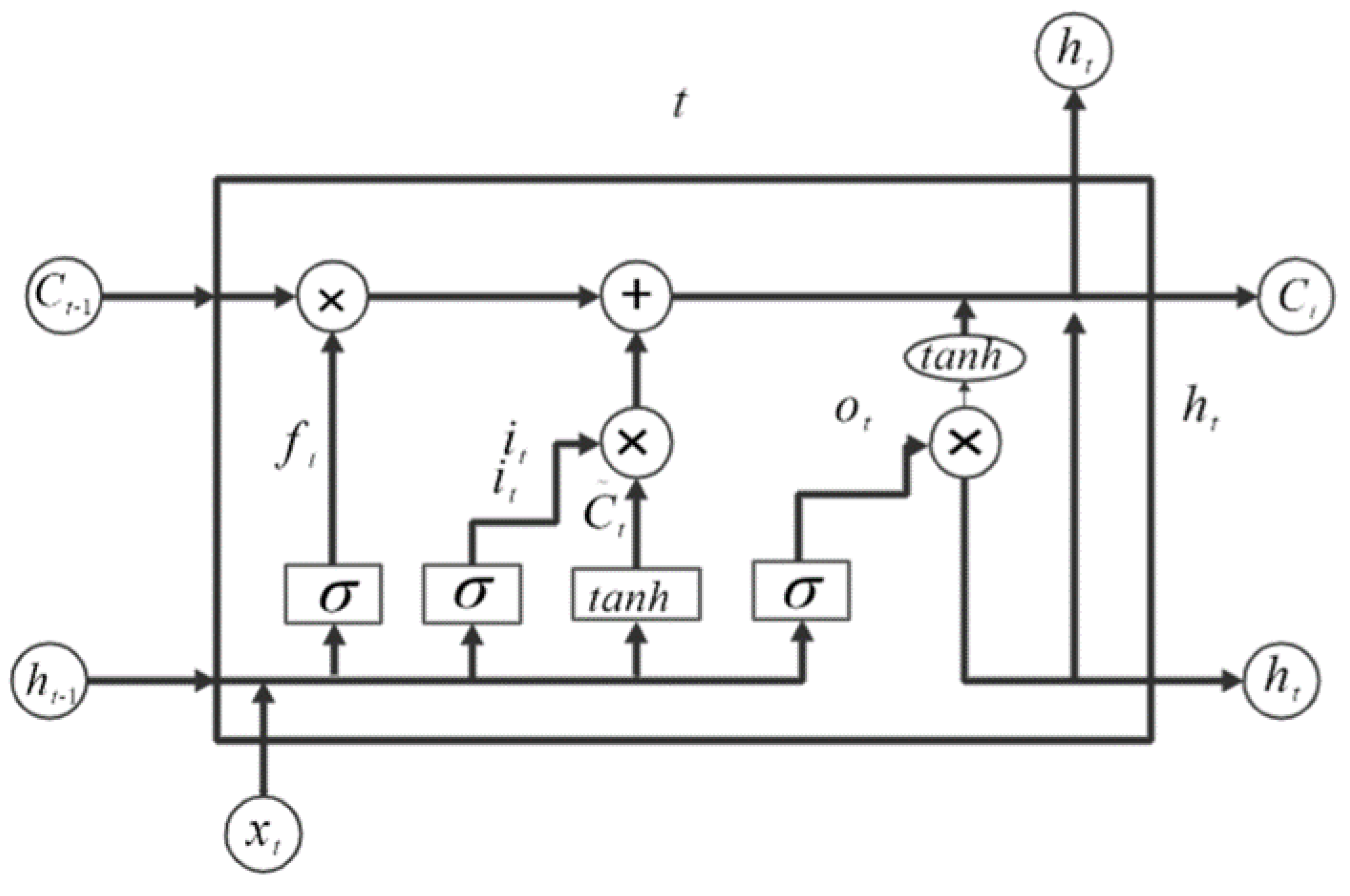
Figure 1. LSTM model diagram.
Atmosphere 13 01476 g001
Figure 2. Spatial distribution and latitudinal variation curve of average CO concentration in different pressure layers in the world from January 2003 to December 2020. (a,b) 850 hPa; (c,d) 500 hPa; (e,f) 100 hPa.
Atmosphere 13 01476 g002
Figure 3. Monthly average variation diagram of global average CO concentration 850 hPa pressure layer from January 2003 to December 2020. (a) Global monthly average in even years; (b) Monthly average in the northern and southern hemispheres.
Atmosphere 13 01476 g003
Figure 4. Line chart and violin chart of the four seasons change of the Global CO concentration 850 hPa pressure layer from 2003 to 2020. (a,d) Global; (b,e) northern hemisphere; (c,f) southern hemisphere.
Atmosphere 13 01476 g004
Figure 5. From 2003 to 2020, the Global CO concentration is 850 hPa, and the atmospheric pressure layer has spatial distribution in even seasons.
Atmosphere 13 01476 g005
Figure 6. Spatial distribution of average CO concentration in different barometric layers in East Asia from September 2002 to December 2021. (a) 850 hPa; (b) 500 hPa; (c) 300 hPa; (d) 150 hPa.
Atmosphere 13 01476 g006
Figure 7. Monthly variation of tropospheric CO concentration in East Asia from 2003 to 2021. (a) Change month by month; (b) Monthly average change over the years.
Atmosphere 13 01476 g007
Figure 8. Annual variation curves of different tropospheric pressure layers in East Asia and the world from 2003 to 2021. (a) 850 hPa; (b) 500 hPa; (c) 300 hPa.
Atmosphere 13 01476 g008
Figure 9. Interannual variation curves of different atmospheric pressure layers and latitudes in East Asia from 2002 to 2020. (a) 850 hPa; (b) 500 hPa; (c) 300 hPa; (d) 150 hPa.
Atmosphere 13 01476 g009
Figure 10. Four season spatial distribution map of different tropospheric pressure layers from 2002 to 2020.
Atmosphere 13 01476 g010
Figure 11. Profile and slope line chart of the world and East Asia from 2003 to 2021. (a) Profile map; (b) Slope map.
Atmosphere 13 01476 g011
Figure 12. Spatial trend of Global CO concentration MK in the middle and upper troposphere from 2003 to 2021. (a,b) 500 hPa; (c,d) 300 hPa; (e,f) 100 hPa. Note: The black dot indicates that the region has passed the 95% significance test.
Atmosphere 13 01476 g012
Figure 13. EOF spatial distribution map and time coefficient map of global tropospheric CO concentration from 2003 to 2021. (a,b) 850 hPa; (c,d) 500 hPa; (e,f) 100 hPa.
Atmosphere 13 01476 g013
Figure 14. Prediction chart of CO time series in the near surface region of the world and East Asia. (a) Global; (b) East Asia.
Atmosphere 13 01476 g014
Figure 15. CO concentration prediction process based on VMD-LSTM.
Atmosphere 13 01476 g015
Figure 16. Decomposition diagram of CO concentration based on VMD decomposition.
Atmosphere 13 01476 g016
Figure 17. Comparison diagram of real value and predicted value of training set and verification set based on VMD-LSTM model. (a) Training set comparison chart; (b) Verification set comparison chart.
Atmosphere 13 01476 g017
Figure 18. The zonal mean concentration distribution of global CO.
Atmosphere 13 01476 g018
Figure 19. Distribution map of zonal mean concentration of CO in East Asia.
Atmosphere 13 01476 g019
Table 1. Mean value, standard deviation, and minimum value and maximum value of CO concentration during the four seasons of the world, northern hemisphere and southern hemisphere from 2002 to 2020.
AreaMean (×10−9)Std (×10−9)Min (×10−9)Max (×10−9)
Global First quarter104.994.1298.88112.97
Global Second quarter92.173.3587.77100.98
Global Third quarter100.513.5695.47106.56
Global Fourth quarter104.603.5498.92110.50
Northern First quarter138.836.52129.21150.97
Northern Second quarter105.434.7698.35118.46
Northern Third quarter112.063.76107.32121.14
Northern Fourth quarter135.215.05127.62142.79
Southern First quarter66.321.6163.9569.55
Southern Second quarter77.011.9874.2281.02
Southern Third quarter87.313.7481.8993.49
Southern Fourth quarter69.872.2267.1173.77
Table 2. From September 2002 to December 2021, the mean, variance, and standard deviation of CO in different pressure layers in East Asia.
Atmospheric Pressure Layer (hPa)Mean (×10−9)Var (×10−9)Std (×10−9)
850125.56246.4315.70
500109.93133.7711.57
30092.0954.417.38
15058.496.962.64
Table 3. Linear fitting of different pressure layers of CO concentration in East Asia and the world from 2003 to 2020.
Atmospheric Pressure Layer (hPa)AreaLinear Fitting Slope (×10−9/a)Correlation Coefficient
850Global−0.552−0.904 **
East Asia−1.129−0.954 **
500Global−0.297−0.662 **
East Asia−0.700−0.825 **
300Global−0.009−0.037
East Asia−0.159−0.417
Note: ** It means passing the significance test of 0.01.
Table 4. Variance contribution and cumulative variance of the first six modes of EOF analysis of CO concentration in different pressure layers of the global troposphere.
ModeEOF1EOF2EOF3EOF4EOF5EOF6Cumulative Variance
850 hPa88.90%3.32%2.65%1.15%0.67%0.55%97.24%
500 hPa56.84%14.95%13.98%3.86%2.05%1.45%93.13%
100 hPa80.72%6.25%4.00%2.22%1.06%0.85%95.10%
Table 5. Evaluation index of global and East Asian near surface CO data sets under three-exponential smoothing model.
AreaMAERMSE R 2
Global1.4691.9150.918
East Asia2.1542.7970.972
Table 6. Correlations between atmospheric temperature, methane, water vapor, and CO in the global lower troposphere from 2003 to 2021.
Atmospheric Pressure Layer (hPa)Atmospheric ParametersCorrelation Coefficient
1000atmospheric temperature−0.829 **
methane−0.419 **
water vapor−0.758 **
925atmospheric temperature−0.801 **
methane−0.538 **
water vapor−0.788 **
850atmospheric temperature−0.749 **
methane−0.529 **
water vapor−0.726 **
Note: ** It means passing the significance test of 0.01.
Publisher’s Note: MDPI stays neutral with regard to jurisdictional claims in published maps and institutional affiliations.