A Deep Learning Micro-Scale Model to Estimate the CO₂ Emissions from Light-Duty Diesel Trucks Based on Real-World Driving

Abstract

On-road carbon dioxide (CO₂) emissions from light-duty diesel trucks (LDDTs) are greatly affected by driving conditions, which may be better predicted with the sequence deep learning model as compared to traditional models. In this study, two typical LDDTs were selected to investigate the on-road CO₂ emission characteristics with a portable emission measurement system (PEMS) and a global position system (GPS). A deep learning-based LDDT CO₂ emission model (DL-DTCEM) was developed based on the long short-term memory network (LSTM) and trained by the measured data with the PEMS. Results show that the vehicle speed, acceleration, VSP, and road slope had obvious impacts on the transient CO₂ emission rates. There was a rough positive correlation between the vehicle speed, road slope, and CO₂ emission rates. The CO₂ emission rate increased significantly when the speed was >5 m/s, especially at high acceleration. The correlation coefficient (R²) and the root mean square error (RMSE) between the monitored CO₂ emissions with PEMS and the predicted values with the DL-DTCEM were 0.986–0.990 and 0.165–0.167, respectively. The results proved that the model proposed in this study can predict very well the on-road CO₂ emissions from LDDTs.

1. Introduction

With the development of the global economy and the increasing demand for energy, the use of fossil fuel, the world’s main energy source, has been increasing yearly [1]. High growth of fossil fuel consumption has led to large amounts of carbon dioxide (CO₂) emissions, which has resulted in a severe ‘greenhouse effect’ [2]. At present, more than 120 countries have proposed carbon neutrality commitments [3], and China has also announced that it will peak carbon emissions in 2030 and achieve carbon neutrality by 2060 [4].

CO₂ emissions from the transport sector have accounted for approximately 22–23% of global anthropogenic CO₂ emissions [5,6,7]. Road transport has become a major source of transport sector CO₂ emissions with the increase of the vehicle population [8]. A recent study reported that CO₂ emissions from the transport sector reached 930 million tons in China in 2020 [9]. Developing an accurate vehicle CO₂ emission model is a primary task for correctly estimating transport CO₂ emissions and also an important basis for formulating policies to reduce transport CO₂ emissions [10,11,12].

Vehicle emission models can be divided into macro- and micro-models according to the input size of the model [13]. The macroscopic model can estimate the total amount of gaseous emissions in a whole area through parameters such as the average speed of vehicles [14,15]. The microscopic model takes the relevant parameters of instantaneous driving conditions of each vehicle as input, such as instantaneous speed and acceleration, to estimate the instantaneous emission rate of pollutants [16,17]. In recent years, there have been many studies of prediction models [18]. Due to the readily available relevant data such as average velocity, macroscopic models have been widely studied [19]. However, such models are not suitable for emission calculation at the micro-level. In order to accurately capture the characteristics of CO₂ emissions from road transport and further reductions in road transport, more accurate micro-scale vehicle CO₂ emission models are needed to be developed [20].

Internationally, traditional micro-scale vehicle emission models have been developed based on statistical methods with a large amount of test data. They have been widely used in the past decades, such as CMEM [21], IVE [22], and MOVES [23]. These models were established by polynomial models with different parameters. They require a great number of parameters, such as the parameters of CMEM including vehicle/technology type, fuel distribution system, emission control technology, vehicle age, vehicle mass, engine displacement, aerodynamic coefficient, air drag coefficient, etc. The model also requires localization of the parameters before it can be used. In practice, the lack of vehicle information and inaccurate parameter localization may cause problems such as insufficient prediction accuracy [24].

With the development of computer hardware, many studies in recent years have focused on the use of machine learning and deep learning to predict exhaust emissions [25]. Junepyo used regression analysis to predict the CO₂ emissions of light-duty diesel trucks (LDDTs), while the determination coefficient (R²) between the regression equation-based CO₂ estimations and real CO₂ measurements was 0.93 [26]. Maksymilian collected real driving emission (RDE) data of hybrid electric vehicles, compared the prediction accuracy of various machine learning models on CO₂ emissions, and Gaussian process regression (GPR) and achieved good results. It has also been found that CO₂ emissions from hybrid electric vehicles are not strictly correlated with speed and acceleration [27]. In recent years, much of the literature adopted the artificial neural networks (ANN) to predict CO₂ emissions with high accuracy. Hashemi and Clark used three parameters, axle speed, torque, and their derivatives, to train an ANN model and predicted CO₂ emissions from heavy-duty diesel vehicles with an accuracy of 0.97 [28]. Jigu et al. integrated an ANN model and a vehicle dynamics model to predict the instantaneous CO₂ emissions of light-duty diesel vehicles [19]. However, the prediction of CO₂ in the study only used two parameters, respectively engine speed and torque, without considering the impact of actual driving conditions on CO₂ emissions. Some of the literature also used ANN to predict the pollutants from vehicle exhaust emissions [29,30,31]. All these studies have a common problem that the models only considered the current engine operating and road conditions in the prediction. However, the exhaust emissions of motor vehicles have long-term temporal dependence. In addition, there is a time error between the measured value of exhaust gas and the measured value of engine operating conditions in the measurement, which still has an impact even after time alignment. Therefore, it is not accurate enough for prediction by only considering the current data.

Traditional ANN do not make inferences about subsequent information based on previous information. Recurrent neural networks (RNN) address this issue, and they are networks with loops in them, allowing information to remain. Since the backpropagation method was adopted in the training of RNN, it might be cause the gradient approaching zero or infinity when the networks were deep. Long short-term memory networks (LSTMs) are a special kind of RNN which address the problem of gradient vanishing and gradient clipping [32]. So, they are more suitable for the prediction of CO₂ emissions of motor vehicles. Tao developed an LSTM-based vehicle emission model to estimate the instantaneous CO₂ emissions of taxicabs and achieved higher accuracy than the state-of-the-art models [18]. Yang found that LSTM had better prediction capability for transient changes in NOx emissions [33]. However, there are few literature examples using sequence models for the estimation of CO₂ emissions from LDDTs.

In this paper, a portable emission measurement system (PEMS) was selected to measure the RDE of two test LDDTs and the vehicle speed, acceleration, and the road slope were calculated based on the data obtained by the onboard global position system (GPS). The second-by-second speed, acceleration, vehicle-specific power (VSP), and road slope were used as the inputs to train an LSTM-based model for CO₂ prediction. The previous 5-s monitored data were used as the input variables, and then transformed by the trained model. Finally, the output of the predicted values of instantaneous rate of CO₂ emissions using the fully connected (FC) layer was carried out.

2. Materials and Methods

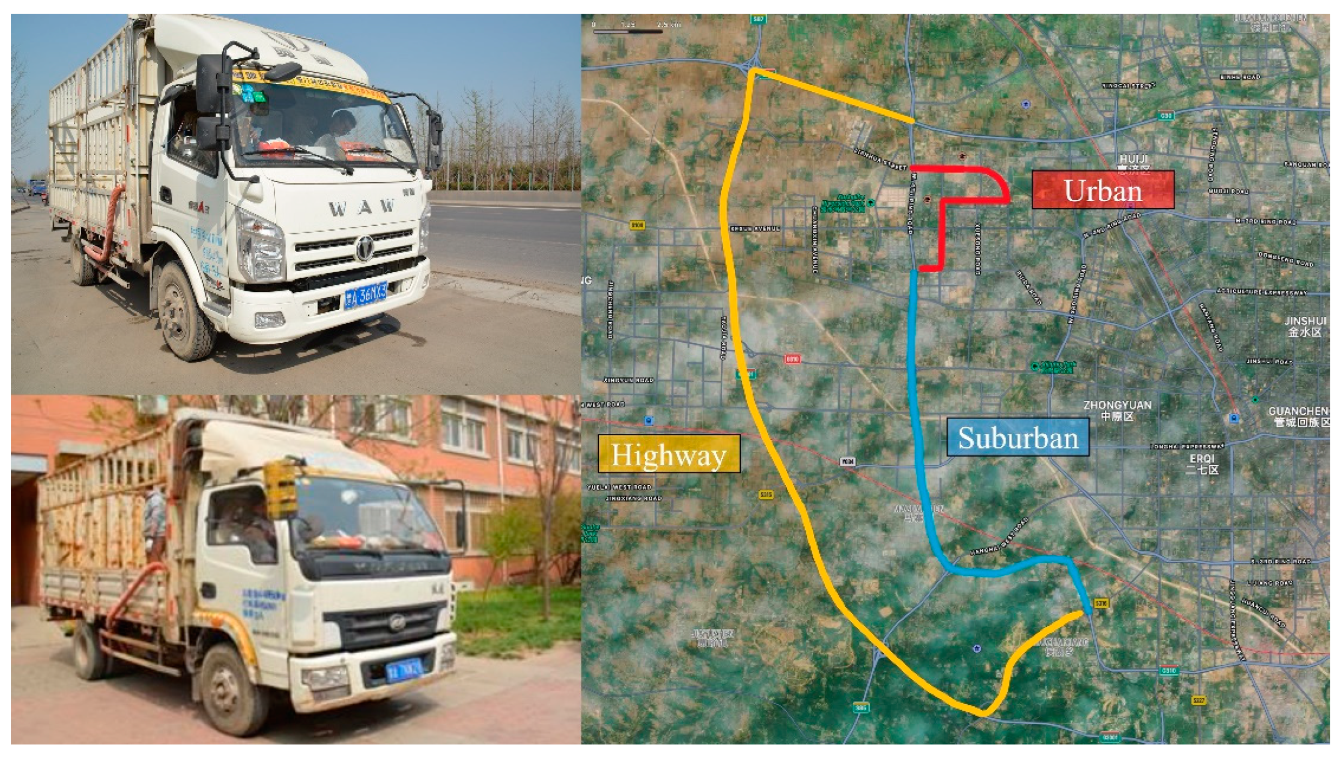
2.1. Test Vehicles and Routes

Two representative diesel trucks, LDDT1 and LDDT2, were selected for real-world CO₂ emission measurement in the experiment. The model years of LDDT1 and LDDT2 were 2016 and 2013, respectively. LDDT1 equipped with a diesel particulate filter (DPF) complied with China IV emission standards and LDDT2 without DPF complied with China III. These vehicles were both in good working conditions with odometer readings of 28,918 km and 94,080 km respectively. More specifications for these test vehicles can be found in our previous study [34]. The fuel used in this study was directly purchased from a local gas station and met the corresponding Automobile diesel fuels (China VI) (GB19147-2016). In order to eliminate the impact of driving habits on CO₂ emissions, both trucks were driven by the owner himself during the experiment.

The transient CO₂ emissions are closely related to the road conditions such as the route type (urban, rural, and highway) and road type (uphill, flat-road, and downhill) [35]. To better reflect the real CO₂ emissions during the actual working in the Central Plains region of China, a test route containing urban (12.4 km), suburban (17.6 km), and highway roads (32.4 km) was designed, as shown in Figure 1. Both LDDT1 and LDDT2 were carried out on the same route, departing from the urban area, circling, and returning to the initial position. The red line represents the urban road, the blue line represents the suburban road, and the yellow line represents the highway.

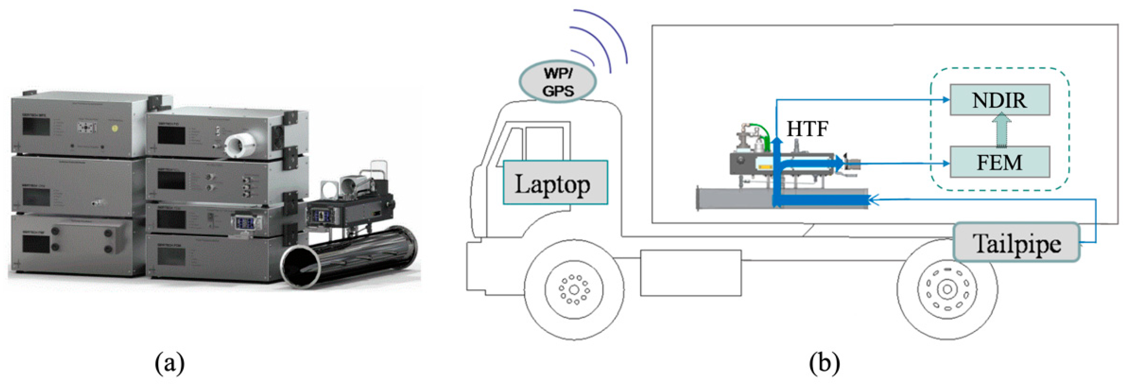
2.2. Test System and Data Analysis

A SEMTECH ECOSTAR PLUS (Sensors Inc., Saline, Michigan, USA) system was used to monitor the CO₂ emissions in this study. The transient CO₂ emissions were monitored with the non-dispersive infrared red (NDIR) method. In addition, the SEMTECH FEM module was used in conjunction with the HTF heating sampling tube to measure the transient flow of the exhaust. Other regulated gaseous pollutants (CO, HC, NOx) were also tested at the same time. This paper only focused on the emission characteristics and the prediction of the CO₂ emissions, and more details can be found in reference [34]. A global positioning system (GPS) was used to record the instantaneous longitude, latitude, and velocity of the vehicle during the test with a spatial resolution of 10 m and velocity of ±1 km/h, respectively. All data were collected at a resolution of 1 Hz and transmitted in real time to a laptop which connected to a gas analyzer. The on-road CO₂ emission data from each truck were monitored by the PEMS, and DL-DTCEM model for each truck which was trained with its own driving data. The on-road CO₂ emission data were divided into the training set and test set according to the ratio of 8:2. Namely, 80% of the data were used for model training, and the remaining 20% of the data were used to evaluate the prediction accuracy of the model. The physical drawing of the PEMS and a schematic of its installation on a LDDT are displayed in Figure 2.

Three running parameters, acceleration, grade, and vehicle specific power (VSP), related to CO₂ emissions could be obtained based on the data recorded by the GPS devices. The acceleration $a_i$ was calculated using the 2-s average of the difference between the previous and subsequent values of velocity $V_i$ as follows.

$$a_i=\frac{1}{2}\cdot \left(V_{i+1}-V_{i-1}\right)$$

(1)

where V_i+1 is the speed of the previous second and V_i-1 is the speed of the subsequent second.

The grade was calculated by the segmented method [36,37], and the grade value was calculated every 50 m in this work, as shown in Equation (2),

$$grade={\displaystyle \sum }_i\mathsf{\Delta }{h}_i$$

(2)

where $\mathsf{\Delta }h$ is the difference of the altitude, $grade$ is the cumulated altitude gain.

For light-duty vehicles (LDV), Jiménez Palacios selected the values of parameters according to the characteristics of LDV in his research [38], and simplified the VSP calculation formula of LDV, as shown in Equation (3).

$$VSP=V_i\cdot \left(1.1\cdot a_i+9.81\cdot grade+0.132\right)+0.000302V_i^3$$

(3)

where V_i is the current vehicle speed, a_i is the current vehicle acceleration, and grade presents road slope.

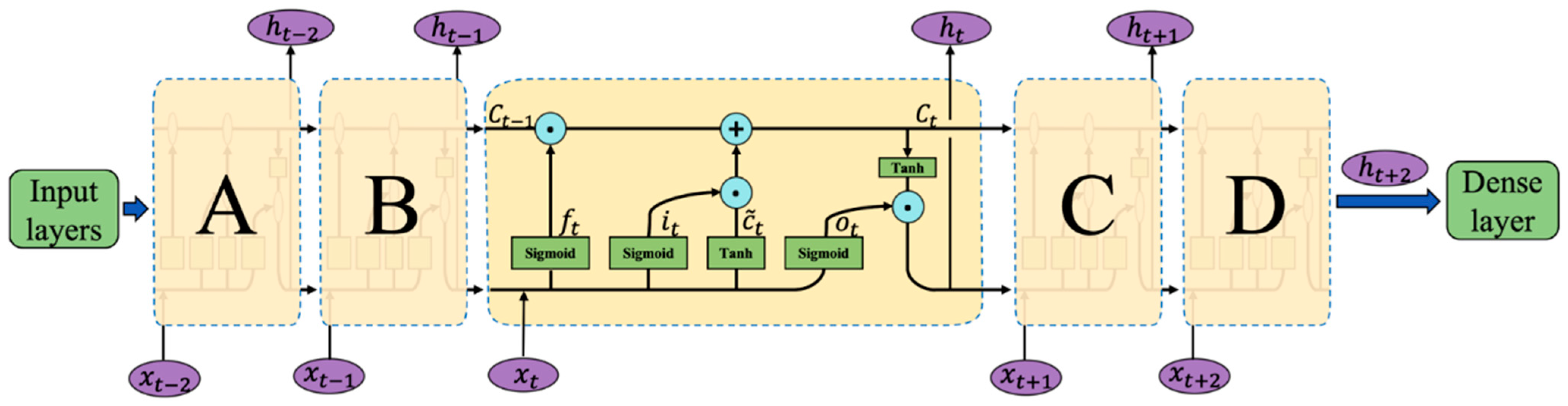
2.3. Deep Learning Model

A deep learning-based CO₂ emission model for LDDTs (DL-DTCEM) based on the sequence model was developed. The input layer preprocessed the data, and the prediction values were output through the dense layer. The input layers first perform data cleansing, then convert the original data to a value between 0 and 1 to improve the prediction accuracy and operation efficiency of the model. Finally, the input layers converted the data into a data structure that could be read by the LSTM module. The LSTMs had a more efficient chain-like structure based on a chain of repeating modules of RNN, as shown in Figure 3. The key to LSTM was the cell state which is a kind of conveyor belt. The horizontal line running through the top of the diagram transports long-term dependency of the data.

Each cell used the forget gate, input gate, and output gate to preserve and update the cell state. As shown in Figure 3, all the middle parts and the A, B, C, D parts had the same cell structure, while the network layer of these cells used the same parameter values. In fact, this was a cell that had been reused at different times. The forget gate was used to decide what information would be discarded from the cell state. When the historical output $h_{t-1}$ moved to the time $t$, it combined with the input $x_t$ at the time $t$. The new vector was operated by $Sigmoid$ function, as shown in Equation (4). Then the result was element-wise multiplicated with the previous cell state $C_{t-1}$ to update the cell state.

$$f_t=Sigmoid\left(W_{xf}{x}_t+W_{hf}{h}_{t-1}+b_f\right)$$

(4)

The input gate determined which new information should be stored in the cell state. The $Sigmoid$ layer determined which information would be updated operated by Equation (5). Next the $Tanh$ layer created a new candidate vector ${\tilde{c}}_t$ operated by Equation (6) that could be added to the state according to Equation (7). Since the operations to update the cell state were minored as linear interactions, the long-term characteristics of the data were protected.

$$i_t=Sigmoid\left(W_{xi}{x}_t+W_{hi}{h}_{t-1}+b_i\right)$$

(5)

$${\tilde{c}}_t=Tanh\left(W_{x\tilde{c}}{x}_t+W_{h\tilde{c}}{h}_{t-1}+b_{\tilde{c}}\right)$$

(6)

$$C_t=f_t\odot C_{t-1}+i_t\odot {\tilde{C}}_t$$

(7)

The output gate could decide which information to be outputted. The output value $h_t$ operated by Equation (8) could be obtained by element-wise multiplying $O_t$ calculated by Equation (9) and the hidden layer output value $g_t$ calculated by Equation (10). Finally, the dense layer outputs the prediction value of CO₂ emissions $y_t$, as calculated according to Equation (11).

$$h_t=o_t\odot g_t$$

(8)

$$o_t=Sigmoid\left(W_{xo}{x}_t+W_{ho}{h}_{t-1}+b_o\right)$$

(9)

$$g_t=Tanh\left(C_t\right)$$

(10)

$$y_t=W_{yh}{h}_t+b_y$$

(11)

2.4. Performance Evaluation

To evaluate the prediction accuracy of the model, the root mean square error (RMSE) and the correlation coefficient (R²) were used as the metrics to evaluate the effectiveness of the DL-DTCEM. RMSE was calculated according to Equation (12).

$$RMSE=\sqrt{1/n{{\displaystyle \sum }}_{t=1}^n{\left(x_t^{C{O}_2}-{\widehat{x}}_t^{C{O}_2}\right)}^2}$$

(12)

where $x_t^{C{O}_2}$ is the observed value, ${\widehat{x}}_t^{C{O}_2}$ represents the predicted value.

3. Results and Discussion

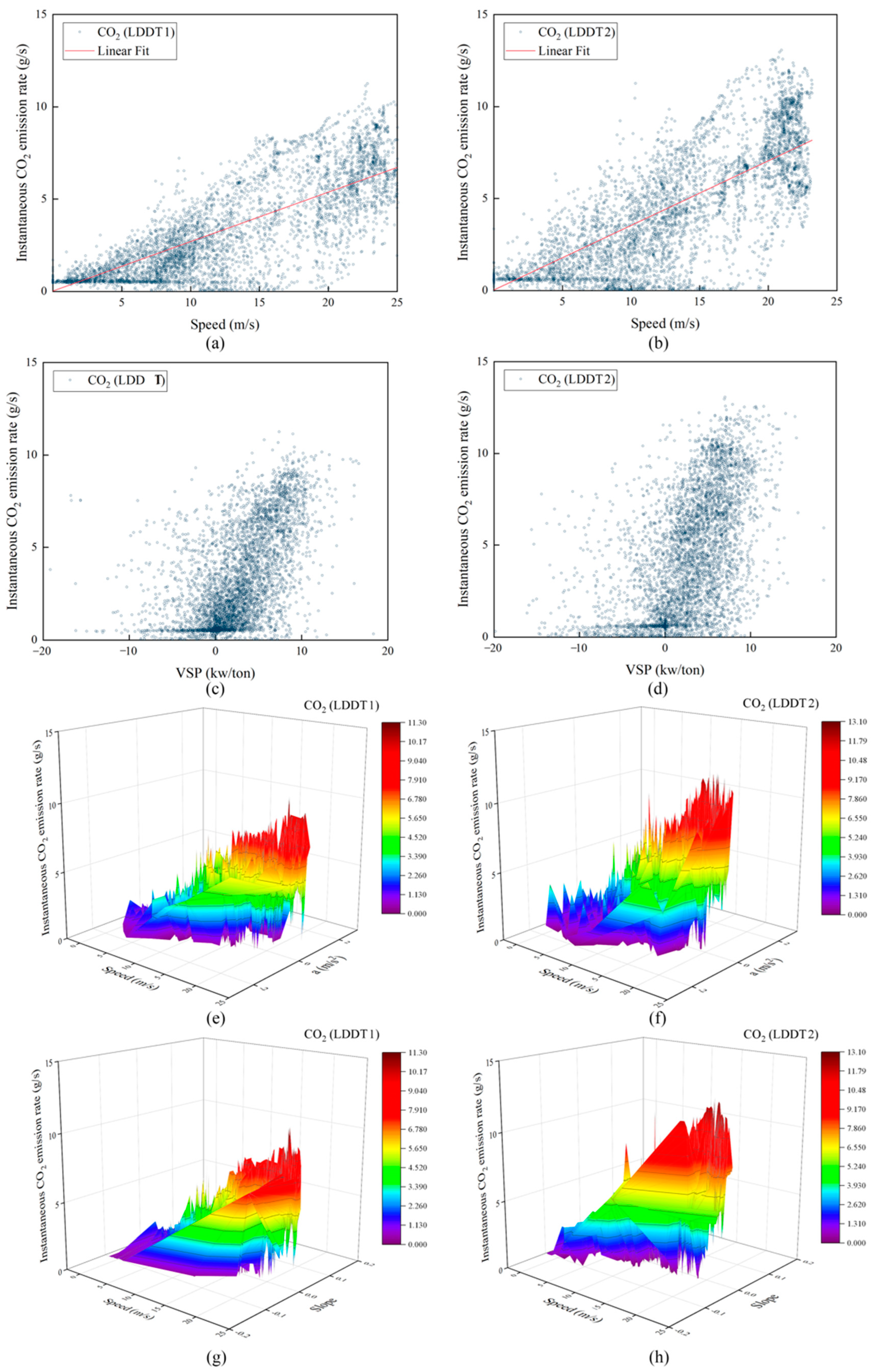
3.1. Impact of Driving Factors on CO₂ Emissions

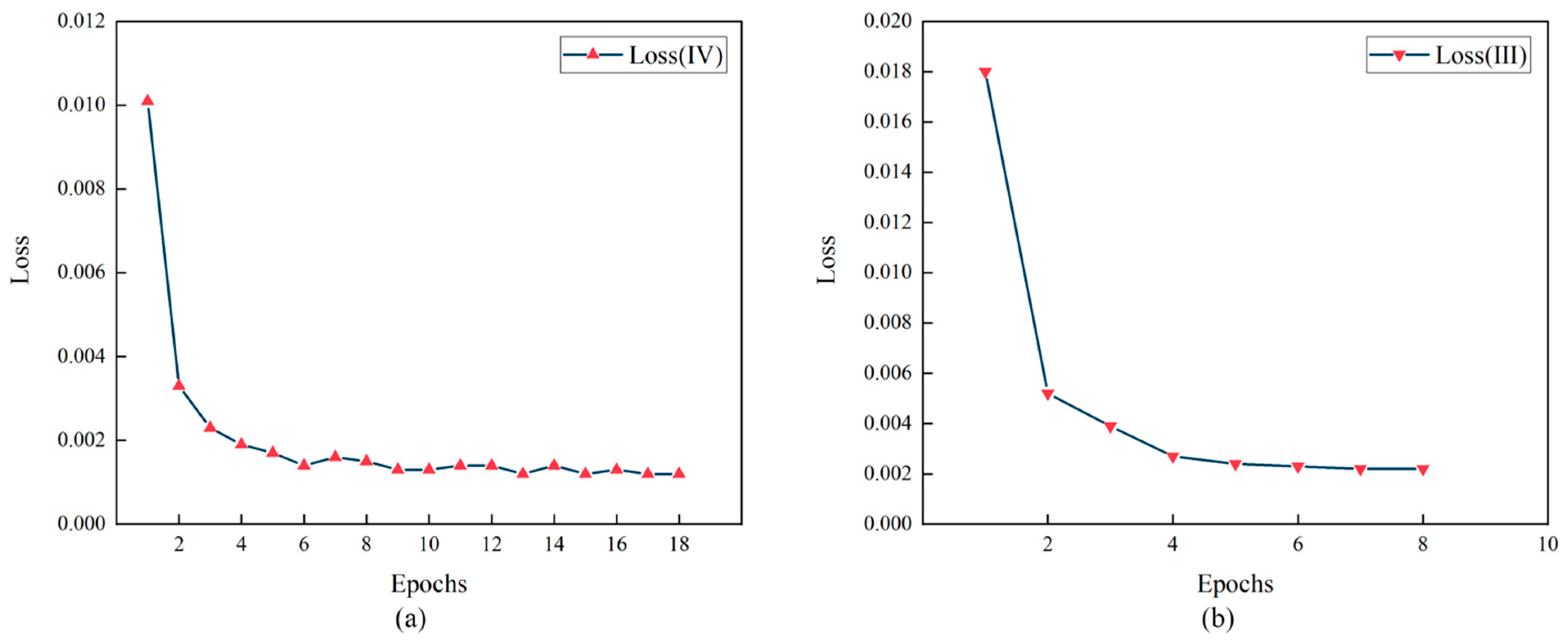
The CO₂ emission rate of vehicles in real-world driving may be affected by many factors. Figure 4 shows the relationship between different driving conditions and CO₂ emission rates. As shown in Figure 4a, b there was a positive correlation between CO₂ emission rate and vehicle speed. When the vehicle speed increased, the CO₂ emission rate increased obviously. Junepyo also measured the average CO₂ emissions at different vehicle speeds and found that the CO₂ emission rates were the highest on the motorway at the fastest speed [26]. At high speeds, the vehicle engine was in a rich combustible state, consuming more fuel to provide enough power output, so the rate of CO₂ emissions rose rapidly.

Figure 4c, d shows the trend of CO₂ emission rate change with VSP. It can be seen that the change law of CO₂ emission rate with VSP of different vehicles was basically the same, mainly distributed in the interval of [−5, 10]. When VSP < 0, it corresponded to the deceleration condition of the vehicle. In this case, the fuel injection was reduced, so the CO₂ emission rate was relatively slow. When VSP > 0, it meant a high concentration air-fuel mixture, and the CO₂ emission rate increased sharply with the increase of VSP. In addition, it can be seen that the CO₂ emission rate rises sharply with rapid acceleration. This finding was consistent with that by Chong et al. conducted in Korea [6]. Therefore, a gentle driving mode can also effectively reduce CO₂ emissions.

The speed of vehicle had a significant influence on the CO₂ emissions and the experimental route was chosen as similar as possible to real driving conditions without deliberately designing the route with a large height drop. It was not appropriate to use acceleration and slope alone to estimate its impact on the vehicle CO₂ emissions. Figure 4e, f shows the relationship between vehicle speed, acceleration, and CO₂ emission rate. Its vertical axes represent the CO₂ emission rate, which is a function of the vehicle speed and acceleration of LDDT1 and LDDT2. It was obvious that there was no clear linear relationship between the vehicle speed, acceleration, and the CO₂ emission rate. When the vehicle speed was larger than 5 m/s and the acceleration was greater than 0.5 m/s², the CO₂ emission rate increased significantly, and the acceleration further increased the CO₂ emission rate as the vehicle speed was high. This result was similar to the finding reported by Zhang with a slightly higher threshold of speed [39].

The vertical axes of Figure 4g,h also represents the CO₂ emission rate, which is a function of the vehicle speed and road slope. It was obvious to find from the figure that when the vehicle speed was the same and the road slope was >0, the CO₂ emission rate increased with the increase of slope. When the road slope was <0, the CO₂ emission rate decreased with the increase of the road slope. This is because much more engine capacity was needed when the vehicle went uphill while it did not need the higher power engine output when the vehicle went downhill.

3.2. Model Training

Vehicle speed, VSP, acceleration, road slope, and historical CO₂ emission rate were used as input variables for model training. Each piece of training data was a two-dimensional array of values of variables in the past five seconds of the current moment. The difference between the predicted value and the observed value at the current moment was used as the basis for model backpropagation, and the model parameters were updated accordingly. In addition, the hyperparameters are also important factors impacting the training effect of the model. The algorithm inherent in Tensorflow, a deep learning framework, was used to automatically select the hyperparameter with the best training effect, then the model was exported as the final DL-DTCEM. The specific hyperparameter information is listed in

Table 1. Specific hyperparameters of DL-DTCEM.

Label	Batch-Size	Epochs	Optimizer
LDDT1	8	18	Adam
LDDT2	8	8	Adam

.

Where, Batch-size denotes the number of training data groups at each training, Epochs represents the iteration times of all training data, and the model Optimizer is used to find the optimal parameters of the model. As shown in Figure 5, with the increase of the number of Epochs, the gap between the predicted value and the observed value of CO₂ gradually decreased, which also meant that the prediction accuracy of the model was gradually improved. The final loss value of prediction of LDDT1 and LDDT2 was 0.0012, 0.0022, respectively.

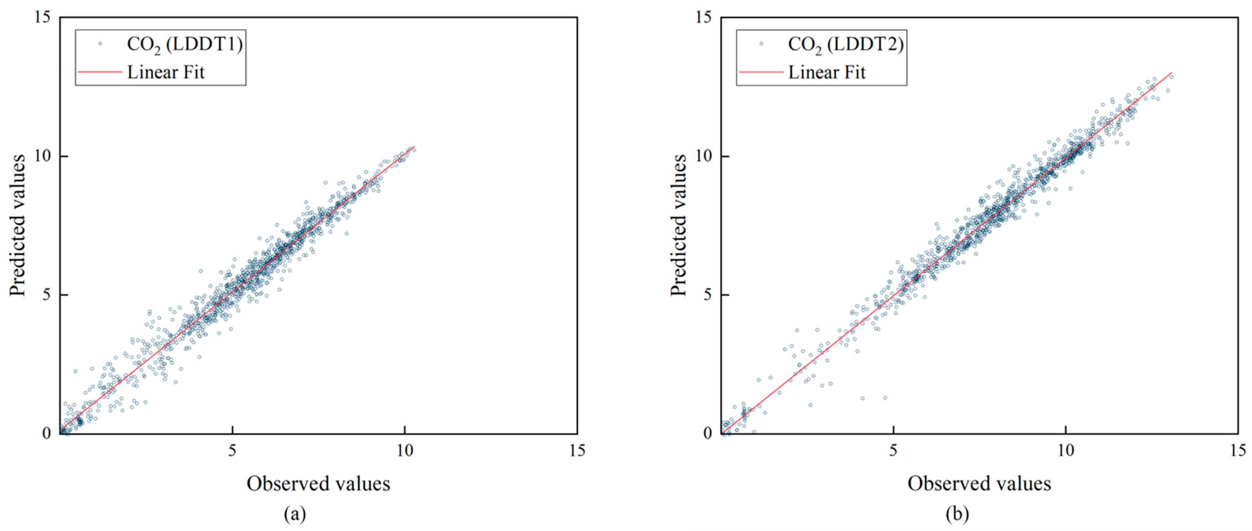
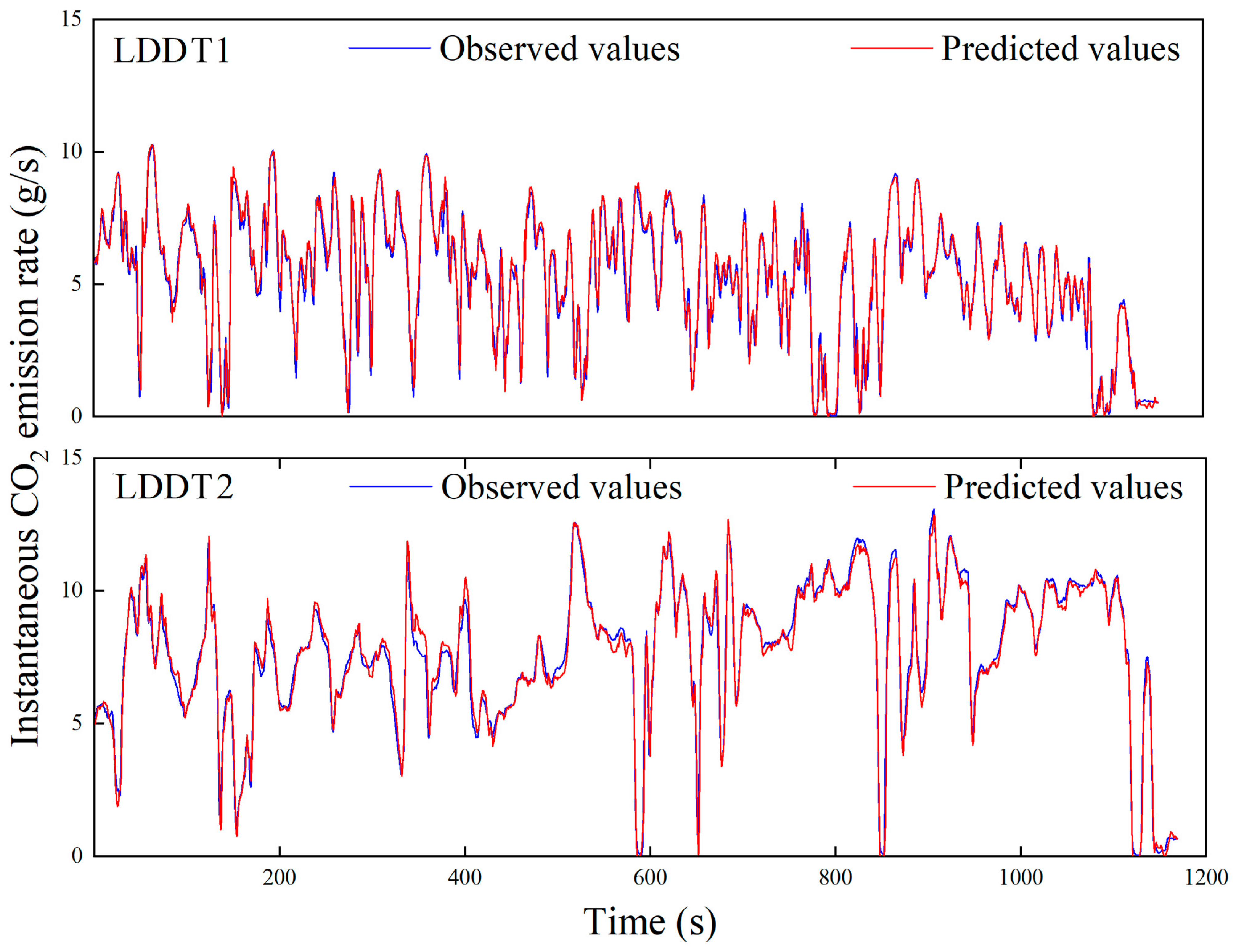
3.3. Model Validation and Discussion

Comparison of the instantaneous CO₂ emission rates of the test set and the predicted values of DL-DTCEM are shown in Figure 6. As can be seen, the instantaneous CO₂ emission rate calculated by our model is very close to the observed values. The RMSE numbers between observed and predicted values of LDDT1 and LDDT2 were 0.1648 and 0.1465, respectively. This means a high prediction accuracy of DL-DTCEM. However, there is a little difference between the predicted values and the observed values at several abrupt points of the CO₂ emission rate, especially in the prediction of LDDT2. This phenomenon could be contributed to the different post-processing for LDDT1 and LDDT2. However, because of the lack of relevant studies, the exact cause of this situation should be investigated further. This also shows that the DL-DTCEM did not learn sufficient about the sudden changing regularity of the CO₂ emission rate.

Figure 7 shows a linear regression analysis of observed CO₂ emissions versus DL-DTCEM predicted CO₂ emission results. The R² values of the CO₂ emission rate prediction values of LDDT1 and LDDT2 are 0.986 and 0.990, respectively. The fit line regression slopes of LDDT1 and LDDT2 are 0.9953 ± 0.005 and 0.9962 ± 0.004, respectively. The R² values between observed and predicted values of traditional, machine learning and other deep learning models with the CO₂ emission rate range from 0.93 to 0.96 [14,18,26]. Through the validation of the CO₂ emission rate prediction results, the DL-DTCEM shows high prediction accuracy, which verifies that the DL-DTCEM can calculate reliable CO₂ emission rates.

4. Conclusions

A PEMS was adopted to investigate the on-road CO₂ emissions from two typical LDDTs, while the information of the longitude, latitude, and elevation data were also collected by a GPS, which was used to calculate the acceleration, VSP, and slope data. The relationship between CO₂ emissions and driving conditions such as vehicle speed, acceleration, VSP, and road slope was also analyzed. A deep learning vehicle CO₂ emission model was developed with the data of the on-road CO₂ emissions and running conditions based on a sequence model. The main findings are as follows.

The vehicle speed, acceleration, VSP, and road slope had obvious impacts on the real-world CO₂ emissions. There was a rough positive correlation between the vehicle speed and CO₂ emission rate. The CO₂ emission rate increased sharply when the vehicle speed was greater than 5 m/s and the acceleration was greater than 0.5 m/s². There was a trend that the instantaneous CO₂ emission rates increased when vehicles accelerated rapidly. The CO₂ emission rates when test vehicles were running uphill was significantly higher than those running downhill. Therefore, driving LDDTs in a smooth way with respect to acceleration and deceleration on the flat road would be beneficial to reduce the transport CO₂ emission.

The DL-DTCEM proposed in this study was able to predict the on-road CO₂ emission rates of vehicles very well. The R² between the CO₂ emission values of LDDT1, LDDT2 predicted by DL-DTCEM and those monitored by the PEMS were 0.986 and 0.990, respectively. The RMSEs for LDDT1 and LDDT2 were 0.1648 and 0.1465, respectively.

In this study, the model was developed based on only two typical vehicles, and the calibration for more and different vehicles should be conducted in future studies. The model achieved good results in CO₂ prediction for LDDTs, and it should be similarly trained to predict other tailpipe pollutants, such as NOx, HC, CO, and PM in future work.

References

1. Wang, L.; Wang, D.; Li, Y. Single-atom Catalysis for Carbon Neutrality. Carbon Energy 2022, 1–59. [Google Scholar] [CrossRef]
2. Smith, I.M. CO2 and Climatic Change: An Overview of the Science. Energy Convers. Manag. 1993, 34, 729–735. [Google Scholar] [CrossRef]
3. Liu, A.; Chen, Y.; Cheng, X. Social Cost of Carbon under a Carbon-Neutral Pathway. Environ. Res. Lett. 2022, 17, 054031. [Google Scholar] [CrossRef]
4. Ma, X.; Huang, G.; Cao, J. The Significant Roles of Anthropogenic Aerosols on Surface Temperature under Carbon Neutrality. Sci. Bull. 2022, 67, 470–473. [Google Scholar] [CrossRef]
5. Oh, Y.; Park, J.; Lee, J.T.; Seo, J.; Park, S. Estimation of CO2 Reduction by Parallel Hard-Type Power Hybridization for Gasoline and Diesel Vehicles. Sci. Total Environ. 2017, 595, 2–12. [Google Scholar] [CrossRef]
6. Chong, H.S.; Park, Y.; Kwon, S.; Hong, Y. Analysis of Real Driving Gaseous Emissions from Light-Duty Diesel Vehicles. Transp. Res. Part D Transp. Environ. 2018, 66, 485–499. [Google Scholar] [CrossRef]
7. Spreen, J.S.; Kadijk, G.; Vermeulen, R.J.; Heijne, V.; Ligterink, N.; Stelwagen, U.; Smokers, R.T.M.; van der Mark, P. Assessment of Road Vehicfle Emissions: Methodology of the Dutch in-Service Testing Programmes. 2016. Available online: https://policycommons.net/artifacts/2180021/assessment-of-road-vehicle-emissions/2935998/ (accessed on 7 September 2022).
8. Liu, Z.; Li, L.; Zhang, Y.-J. Investigating the CO2 Emission Differences among China’s Transport Sectors and Their Influencing Factors. Nat. Hazards 2015, 77, 1323–1343. [Google Scholar] [CrossRef]
9. Teng, W.; Zhang, Q.; Liu, F.; Ying, G. The Progress in the Research on Estimation of Vehicle Carbon Emission in China. J. South China Norm. Univ. (Nat. Sci. Ed.) 2022, 54, 83–92. (In Chinese) [Google Scholar]
10. Matteo, B.; Nanni, M.; Pappalardo, L. Gross Polluters and Vehicle Emissions Reduction. Nat. Sustain. 2022, 5, 699–707. [Google Scholar]
11. Emrah, D.; Bektaş, T.; Laporte, G. A Review of Recent Research on Green Road Freight Transportation. Eur. J. Oper. Res. 2014, 237, 775–793. [Google Scholar]
12. Marina, K.; Fontaras, G.; Ntziachristos, L.; Bonnel, P.; Samaras, Z.; Dilara, P. Use of Portable Emissions Measurement System (PEMS) for the Development and Validation of Passenger Car Emission Factors. Atmos. Environ. 2013, 64, 329–338. [Google Scholar]
13. Delia, A.; Weilenmann, M.; Soltic, P. Towards Accurate Instantaneous Emission Models. Atmos. Environ. 2005, 39, 2443–2449. [Google Scholar]
14. Hao, L.; Hao, C.; Ji, L.; Yin, H.; Zhang, W.; Wang, X.; Liu, J. Statistical Modeling of Exhaust Emissions from Gasoline Passenger Cars. J. Beijing Inst. Technol. 2021, 30, 52–63. [Google Scholar]
15. He, Z.; Zhang, W.; Jia, N. Estimating Carbon Dioxide Emissions of Freeway Traffic: A Spatiotemporal Cell-Based Model. IEEE Trans. Intell. Transp. Syst. 2020, 21, 1–11. [Google Scholar] [CrossRef]
16. Michail, M.; Mattas, K.; Mogno, C.; Ciuffo, B.; Fontaras, G. The Impact of Automation and Connectivity on Traffic Flow and CO2 Emissions. A Detailed Microsimulation Study. Atmos. Environ. 2020, 226, 117399. [Google Scholar]
17. Christina, Q.; Borge, R.; Pérez, J.; Lumbreras, J.; de la Paz, D.; de Andrés, J.M. Microscale Traffic Simulation and Emission Estimation in a Heavily Trafficked Roundabout in Madrid (Spain). Sci. Total Environ. 2016, 566–567, 416–427. [Google Scholar]
18. Tao, J.; Zhang, P.; Chen, B. A Microscopic Model of Vehicle CO2 Emissions Based on Deep Learning—A Spatiotemporal Analysis of Taxicabs in Wuhan, China. IEEE Trans. Intell. Transp. Syst. 2022, 1–10. [Google Scholar] [CrossRef]
19. Jigu, S.; Yun, B.; Park, J.; Park, J.; Shin, M.; Park, S. Prediction of Instantaneous Real-World Emissions from Diesel Light-Duty Vehicles Based on an Integrated Artificial Neural Network and Vehicle Dynamics Model. Sci. Total Environ. 2021, 786, 147359. [Google Scholar]
20. Jian, H.; Wang, Y.; Liu, Z.; Guan, B.; Long, D.; Du, X. On Modeling Microscopic Vehicle Fuel Consumption Using Radial Basis Function Neural Network. Soft Comput. 2015, 20, 2771–2779. [Google Scholar]
21. U.S. Environmental Protection Agency. Comprehensive Modal Emissions Model (CMEM) Version 2.0: User’ S Guide; U.S. Environmental Protection Agency: Washington, DC, USA, 2004. [Google Scholar]
22. University of California at Riverside. IVE Model User’ S Manual Version 1.1.1.; University of California at Riverside: Riverside, CA, USA, 2004. [Google Scholar]
23. U.S. Environmental Protection Agency. S. Environmental Protection Agency. Technical Guidance on the Use of MOVES2010 for Emission Inventory Preparation in State Implementation Plans and Transportation Conformity; U.S. Environmental Protection Agency: Washington, DC, USA, 2010. [Google Scholar]
24. Jigu, S.; Yun, B.; Kim, J.; Shin, M.; Park, S. Development of a Cold-Start Emission Model for Diesel Vehicles Using an Artificial Neural Network Trained with Real-World Driving Data. Sci. Total Environ. 2021, 806, 151347. [Google Scholar]
25. Zhong, S.; Zhang, K.; Bagheri, M.; Burken, J.G.; Gu, A.; Li, B.; Ma, X.; Marrone, B.L.; Ren, Z.J.; Schrier, J.; et al. Machine Learning: New Ideas and Tools in Environmental Science and Engineering. Environ. Sci. Technol. 2021, 55, 12741–12754. [Google Scholar] [CrossRef]
26. Junepyo, C.; Park, J.; Lee, H.; Chon, M.S. A Study of Prediction Based on Regression Analysis for Real-World CO2 Emissions with Light-Duty Diesel Vehicles. Int. J. Automot. Technol. 2021, 22, 569–577. [Google Scholar]
27. Maksymilian, M.; Jaworski, A.; Kuszewski, H.; Woś, P.; Campisi, T.; Lew, K. The Development of CO2 Instantaneous Emission Model of Full Hybrid Vehicle with the Use of Machine Learning Techniques. Energies 2021, 15, 142. [Google Scholar]
28. Hashemi, N.; Clark, N.N. Artificial Neural Network as a Predictive Tool for Emissions from Heavy-Duty Diesel Vehicles in Southern California. Int. J. Engine Res. 2007, 8, 321–336. [Google Scholar] [CrossRef]
29. Pai, P.S.; Rao, B.S. Artificial Neural Network Based Prediction of Performance and Emission Characteristics of a Variable Compression Ratio CI Engine Using WCO as a Biodiesel at Different Injection Timings. Appl. Energy 2011, 88, 2344–2354. [Google Scholar]
30. Cai, M.; Yin, Y.; Xie, M. Prediction of Hourly Air Pollutant Concentrations near Urban Arterials Using Artificial Neural Network Approach. Transp. Res. Part D Transp. Environ. 2009, 14, 32–41. [Google Scholar] [CrossRef]
31. Jaikumar, R.; Nagendra, S.S.; Sivanandan, R. Modeling of Real Time Exhaust Emissions of Passenger Cars Under heterogeneous Traffic Conditions. Atmos. Pollut. Res. 2016, 8, 80–88. [Google Scholar] [CrossRef]
32. Hamrani, A.; Akbarzadeh, A.; Madramootoo, C.A. Machine Learning for Predicting Greenhouse Gas Emissions from Agricultural Soils. Sci. Total Environ. 2020, 741, 140338. [Google Scholar] [CrossRef]
33. Yu, Y.; Wang, Y.; Li, J.; Fu, M.; Shah, A.N.; He, C. A Novel Deep Learning Approach to Predict the Instantaneous NOx Emissions from Diesel Engine. IEEE Access 2021, 9, 11002–11013. [Google Scholar] [CrossRef]
34. Mei, H.; Wang, L.; Wang, M.; Zhu, R.; Wang, Y.; Li, Y.; Zhang, R.; Wang, B.; Bao, X. Characterization of Exhaust CO, HC and NOx Emissions from Light-Duty Vehicles under Real Driving Conditions. Atmosphere 2021, 12, 1125. [Google Scholar] [CrossRef]
35. Chong, H.; Kwon, S.; Lim, Y.; Lee, J. Real-World Fuel Consumption, Gaseous Pollutants, and CO2 Emission of Light-Duty Diesel Vehicles. Sustain. Cities Soc. 2019, 53, 101925. [Google Scholar] [CrossRef]
36. Gallus, J.; Kirchner, U.; Vogt, R.; Benter, T. Impact of Driving Style and Road Grade on Gaseous Exhaust Emissions of Passenger Vehicles Measured by a Portable Emission Measurement System (PEMS). Transp. Res. Part D Transp. Environ. 2017, 52, 215–226. [Google Scholar] [CrossRef]
37. Boroujeni, B.Y.; Frey, H.C.; Sandhu, G.S. Road Grade Measurement Using in-Vehicle, Stand-Alone GPS with Barometric Altimeter. J. Transp. Eng. 2013, 139, 605–611. [Google Scholar] [CrossRef]
38. Jiménez-Palacios, L. Understanding and Quantifying Motor Vehicle Emissions with Vehicle Specific Power and TILDAS Remote Sensing. 2009. Available online: http://cires1.colorado.edu/jimenez/Papers/Jimenez_PhD_Thesis.pdf (accessed on 7 September 2022).
39. Zhang, Y.; Zhou, R.; Peng, S.; Mao, H.; Yang, Z.; Andre, M.; Zhang, X. Development of Vehicle Emission Model Based on Real-Road Test and Driving Conditions in Tianjin, China. Atmosphere 2022, 13, 595. [Google Scholar] [CrossRef]
Figure 1. The test photos of two vehicles and the routes designed for the real-driving CO2 emission tests.
Atmosphere 13 01466 g001
Figure 2. (a) PEMS equipment; (b) technical schematic diagram. NDIR (non-dispersive infrared red analyzer); HTF and FEM modules, used for the measurement of exhaust flow.
Atmosphere 13 01466 g002
Figure 3. The structure of the deep learning-based CO2 emission model (DL-DTCEM).
Atmosphere 13 01466 g003
Figure 4. The typical relationship between different driving conditions and CO2 emission rate; (a,b) Relationship between vehicular speed and CO2 emission rate; (c,d) Relationship between vehicular VSP and CO2 emission rate; (e,f) Relationship between vehicular speed, acceleration and CO2 emission rate; (g,h) Relationship between vehicular speed, road slope and CO2 emission rate.
Atmosphere 13 01466 g004
Figure 5. The training loss values of DL-DTCEM: (a) loss values of LDDT1 prediction, (b) loss values of LDDT2 prediction.
Atmosphere 13 01466 g005
Figure 6. Comparison of DL-DTCEM predicted CO2 emission rate with observed data.
Atmosphere 13 01466 g006
Figure 7. Linear regression between observed values and DL-DTCEM predicted values: (a) CO2 emissions of LDDT1, (b) CO2 emissions of LDDT2.
Atmosphere 13 01466 g007