Article

Air Quality and Traffic Trends in Cincinnati, Ohio during the COVID-19 Pandemic

by
Rachel Helen Tumbleson
and
Simone Balachandran
*
Department of Chemical and Environmental Engineering, College of Engineering and Applied Science, University of Cincinnati, Cincinnati, OH 45219, USA
*
Author to whom correspondence should be addressed.
Atmosphere 2022, 13(9), 1459; https://doi.org/10.3390/atmos13091459
Submission received: 2 August 2022 / Revised: 28 August 2022 / Accepted: 2 September 2022 / Published: 8 September 2022
(This article belongs to the Section Air Quality)

Abstract

:
During 2020, the stay-at-home order mandated in response to the COVID-19 pandemic led to significant changes in traffic volumes in Cincinnati, OH. Air pollutant concentrations (PM2.5, black carbon (BC), carbon monoxide (CO), nitrogen dioxide (NO2), nitrogen dioxide (NOX), and ozone (O3)) monitored at two ground monitoring sites in the city of Cincinnati were analyzed intra-annually in 2020 to quantify if the stay-at-home order impacted air quality. Interannual analyses were also conducted to evaluate differences in 2020 data versus historical years (2016–2019). Traffic volume data were also analyzed, where it was observed that, compared to pre-pandemic 2020, total traffic counts decreased by up to 26.41% during Ohio’s stay-at-home order, while heavy-duty vehicle traffic increased by up to 26.95% during the latter half of 2020. Statistical analysis indicated nonuniform changes in air pollutant concentrations at both sites throughout 2020. During the lockdown period at the central monitoring site, PM2.5 increased by 9%, while NO2 decreased by 30% compared to pre-pandemic concentrations in 2020. For BC and CO, there were no significant changes.

1. Introduction

On-road mobile vehicles are major sources of fine particulate matter with an aerodynamic diameter less than 2.5 microns (PM2.5). Compared to compounds of larger size, PM2.5 has been associated with numerous health effects. The large surface area exhibited by fine PM2.5 allows for increased adsorption of toxic compounds [1]. Additionally, it is especially damaging to health because it can create health complications from both short- and long-term exposures [2,3,4,5]. Epidemiological studies have also shown that exposure to PM2.5 has been associated with cardiopulmonary morbidity and mortality [6], as well as harmful birth effects [7].
The health effects of air pollution have been studied in Cincinnati for numerous years. This has included PM2.5 modeling [8], speciation analysis [9], and its association with pediatric asthma [10,11] and stillbirths [12]. Additionally, the region’s NOX–VOC and ozone relationships have been of interest [13] especially because, in recent years (2018–2021), Hamilton County (the county in which the city of Cincinnati resides) has been considered in marginal nonattainment for 8 h ozone concentrations based on the 2015 standard of 0.070 ppm. The EPA announced on 9 June 2022 that Hamilton County reached attainment standards for O3. Nevertheless, there is considerable ongoing work in Cincy with regard to the impact of air pollution on health.
Mobile sources are a major contributor to all six criteria pollutants for which the US EPA has established National Ambient Air Quality Standards (NAAQS), which set allowable limits on atmospheric concentrations of carbon monoxide (CO), lead, nitrogen dioxide (NO2), ozone (O3), PM2.5, PM10 (particulate matter with an aerodynamic diameter less than 10 μm), and sulfur dioxide (SO2). These air pollutants are emitted directly into the air and are also formed through chemical reactions in the atmosphere. Ground-level O3, for example, (the main component of smog), is formed through photochemical reactions between oxides of nitrogen (NOX) and volatile organic compounds (VOCs). In addition to the six criteria air pollutants, mobile sources emit a significant amount of black carbon (BC) and elemental carbon (EC), both of which are components of PM2.5. BC and EC differ as a function of their measurement technique. BC refers to the light-absorbing component of carbonaceous aerosols and is determined using optical techniques. In contrast, the EC is a refractory component of PM2.5 and is measured using a thermo-optical technique under oxidizing conditions [14]. BC and EC are short-lived pollutants that are emitted when fossil and biomass fuels are combusted, and they are important to air quality due to their association with harmful health effects and contribution to climate change through having a positive radiative forcing.
Given the importance of mobile sources to air quality, there has been much interest in the research community to quantify the effects of the policies implemented in response to the SARS-CoV-2 pandemic. Cincinnati is the third largest city in the state of Ohio and a major transportation hub in the Midwest. It is situated in the Ohio River Valley with a metropolitan population of approximately 2,256,000. Two major interstates, I-75 and I-71, pass through it. I-75 is one of the largest north–south interstate roadways in the US, connecting southern Florida to the upper peninsula of Michigan. I-71 is a smaller-scale interstate highway, connecting Cleveland, Ohio with Louisville, Kentucky. The Ohio–Indiana–Kentucky tri-state area also features an auxiliary interstate highway, I-275.
In December 2019, the first cases of the novel coronavirus SARS-CoV-2 were discovered. The United States (US) has seen about 57.9 million cases and approximately 1.02 million deaths attributed to COVID-19 as of July 2022. Illness severity can be intensified when infected individuals have chronic lung diseases such as asthma or chronic obstructive pulmonary disease (COPD), as well as heart conditions, which are associated with exposure to poor air quality [15,16]. Risk of death from COVID-19 is also higher in individuals aged >70, males, some ethnic groups, and economically disadvantaged populations.
The first three cases of COVID-19 contracted by Ohioans were reported on 9 March with the first death reported 20 March [17]. Shortly after, the World Health Organization declared the virus a pandemic on 11 March 2020. During this time, the State of Ohio began to issue closings of numerous public places. Mass gatherings were prohibited on 12 March, K-12 schools were ordered to close 14 March, sit-down dining was banned on 15 March, salons were shut down on 19 March, and entertainment venues were closed on 21 March [17]. Following these events, Governor Mike DeWine issued a stay-at-home order for the entire state of Ohio that remained effective from 23 March to 1 May. All citizens were to remain at home unless required to take part in essential work or activity. Retail stores were allowed to open on 12 May. Salons, barber shops, and spas could open on 15 May. Lastly, bars and restaurants were opened on 20 May.
Since the onset of the COVID-19 pandemic, several studies have investigated the association between air quality and COVID-19 mortality. In 92 Western counties in the United States, there were approximately 20,000 extra COVID-19 infections and 750 deaths associated with exposure to elevated levels of PM2.5 during wildfires in 2020 [18]. Furthermore, exposure to poor air quality over time (2000–2016) was associated with an 8% increase in COVID-19 elated mortality for every 1 ug/m3 increase in PM2.5 in the United States [19]. Similarly, an increase in exposure to hazardous air pollutants (HAPs) was linked with a 9% increase in death among patients with COVID-19 [20]. Moreover, a study that calculated the COVID-19 mortality fraction attributed to air pollution found that PM2.5 pollution contributed to 7–33% of COVID-19 deaths worldwide and 6–39% in North America [21].
As stay-at-home orders were mandated around the world in an attempt to prevent the spread of the virus, a number of studies analyzed the impact to air quality due to decreased traffic. A study spanning the entire US found an approximate 25.5% reduction in NO2 compared to historical (2017–2019) levels, as well as a reduction in PM2.5 (4.45%) [22]. Chicago, the third largest metro area in the US, saw no change in air quality during the pandemic which suggested that the diesel-fueled long-haul rail operations that persisted throughout the pandemic may have been the reason for lack of such a change [23]. In Pittsburgh, it was found that NO2 and PM10 concentrations decreased at many of the analyzed sites; however, decreases in PM2.5 pollution varied by site [24]. A nationwide study looking into the effects of stay-at-home orders on air quality chose Cincinnati’s Taft site as one of the 28 N-Core sites analyzed. It was found that this site saw a statistically significant increase (18%) in PM10 when comparing 25 January through 7 March 2020, versus 15 March through 25 April 2020, and a statistically insignificant increase of 19% in PM2.5 was found over this time period [25].
This study aims to analyze the effects of the COVID-19 pandemic on Cincinnati’s air quality, specifically for PM2.5, BC, CO, NOX, NO2, and O3. Air pollutant data were gathered from the central monitoring site (Taft), as well as a site near a major interstate (Near Road). Traffic data were also analyzed during 2020 to identify time periods where traffic volumes were most impacted by COVID-19 policies. Lastly, the impact of meteorology was evaluated by quantifying the atmospheric boundary layer height (ABL), as well as analyzing trends in ambient temperate, pressure, relative humidity, and scalar wind speed.

2. Materials and Methods

2.1. Air Quality Data and Site Information

Ground-level air pollution data from 1 January 2016 through 11 December 2020 was analyzed from two monitoring locations in Cincinnati: the Near Road site and the Taft site, a US EPA N-Core site (Table 1). The Near Road site is located adjacent to the I-75, approximately 3 miles from downtown, and the Taft site is located about half a mile from the I-71 and approximately 2.5 miles from downtown (Figure 1). Air pollutant data were provided by the region’s Southwest Ohio Air Quality Agency (SWOAQA). One hour average air quality data analyzed from the Taft site included BC, PM2.5, CO, NOX, and O3. One hour average air quality data from the Near Road site included BC, PM2.5, NOX, and CO. All air pollutant data were preprocessed to remove data with negative and zero values.

2.2. Traffic Count Data and Site Information

The Ohio Department of Transportation (ODOT) has numerous traffic count monitors along major roadways in the greater Cincinnati region. Each traffic monitoring site records traffic counts according to a size classification. Classifications in this work included vehicles 0–7 ft (Federal Class 1), vehicles 7–29 ft (Federal Classes 2–3), and vehicles greater than 29 ft (Federal Classes 4–13). Federal Class 1 consists of motorcycles, Federal Classes 2–3 comprise cars and pickup trucks, and Federal Classes 4–13 include single unit and combination unit trucks. Total traffic counts of vehicles of all sizes were also included.
Three traffic sites of interest were included in this study, referred to as the Northgate site, Mt. Healthy site, and Near Road site (Figure 1). The Northgate and Mt. Healthy sites use a Wavetronix radar to document the total length of each vehicle. ODOT calibrates these monitors manually by reviewing 4–8 h of video, ensuring to include peak traffic times, and hand counts are compared to values collected by the Wavetronix head. The Near Road traffic monitoring site is a weigh-in-motion site, where inductive loops and piezoelectric sensors work together to determine the exact length of the axel of the vehicle and then assign it to a specific federal classification bin on the basis of a classification tree.

2.3. Predicting 2020 Traffic Counts at Near Road Site

In order to investigate the connection between traffic and air quality during Ohio’s stay-at-home order, traffic volumes in 2020 at the Near Road site were modeled using linear regression since the traffic count monitor at the Near Road site was only operational from May 2017 to February 2019. The Northgate and Mt. Healthy sites were operational during this same time period and continued to measure traffic volumes.
Therefore, traffic volume data for each vehicle classification type at the Near Road site were regressed on traffic data from the Northgate and Mt. Healthy sites, which were treated as the independent variables. Linear regression was conducted for each classification type, as well as total traffic, for data from May 2017 to February 2019.

2.4. Air Quality Data Analysis

Predicted traffic volumes were used to bin air quality data in 2020 into several time periods: 1 January–22 March (the start of the year up to the day before the stay-at-home order was enacted), 23 March–10 April (first half of the stay-at-home order), 23 March–1 May (entirety of stay-at-home-order), 23 March–20 May (entirety of stay-at-home order through the full opening of Ohio’s public venues), 23 March–30 June (entirety of stay-at-home order through the full opening of Ohio’s public venues and just before traffic seemed to return to normal), and 1 July–11 December (post stay-at-home order and once traffic seemed to return to normal). To determine whether Ohio’s stay-at-home order influenced any statistically significant differences in Cincinnati’s air quality, analysis of variance (ANOVA) was utilized to test for differences in mean pollutant concentration across these six time periods of interest. ANOVA tests were conducted on an interannual basis to compare 2020 air pollutant concentrations to historical data (2016–2019), as well as on an intra-annual basis for 2020 to compare pre-pandemic versus the time periods determined from the predicted traffic volumes. Statistical analyses included the Tukey test to examine the degree of difference in mean pollutant concentration between each pairwise comparison and the Student’s t-test to compare differences in means.

2.5. Meterological Analysis

Daily meteorological data (ambient temperature, ambient pressure, ambient relative humidity, and scalar wind speed) at the Near Road site were obtained from the US EPA for every day 2016 through 2020. Metrological data were grouped into the same six time periods as the air pollutant data and were qualitatively analyzed to determine if any major meteorological phenomena were present thought could significantly impact air pollution.
Additionally, the height of the atmospheric boundary layer (ABL) was estimated using the Bulk Richardson Number, as seen in Equation (1) [27]. The calculation of the ABL height was conducted to identify possible temperature inversions which can limit the amount of atmospheric mixing and lead to the accumulation of pollutants in an affected region.
RiB = (gz (θv − θs))/(θs (u2 + v2)),
where θs is the virtual potential temperature at the surface, and θv is the virtual potential temperature at height z. u and v are the horizontal wind components at height z; g is the gravitational acceleration. Two atmospheric sounding data runs from Wilmington, Ohio (one at 8 p.m. and the other at 8 a.m.) published by the University of Wyoming were used to calculate two ABL heights for each day over the year 2020. The top of the ABL was determined as the height at which the Bulk Richardson Number reaches a critical value (0.2) [27]. This technique has been shown to be one of the best methods for the climatological analysis of the ABL because of its applicability for both stable and convective boundary layers [28].

3. Results

3.1. Traffic Counts at Northgate and Mt. Healthy

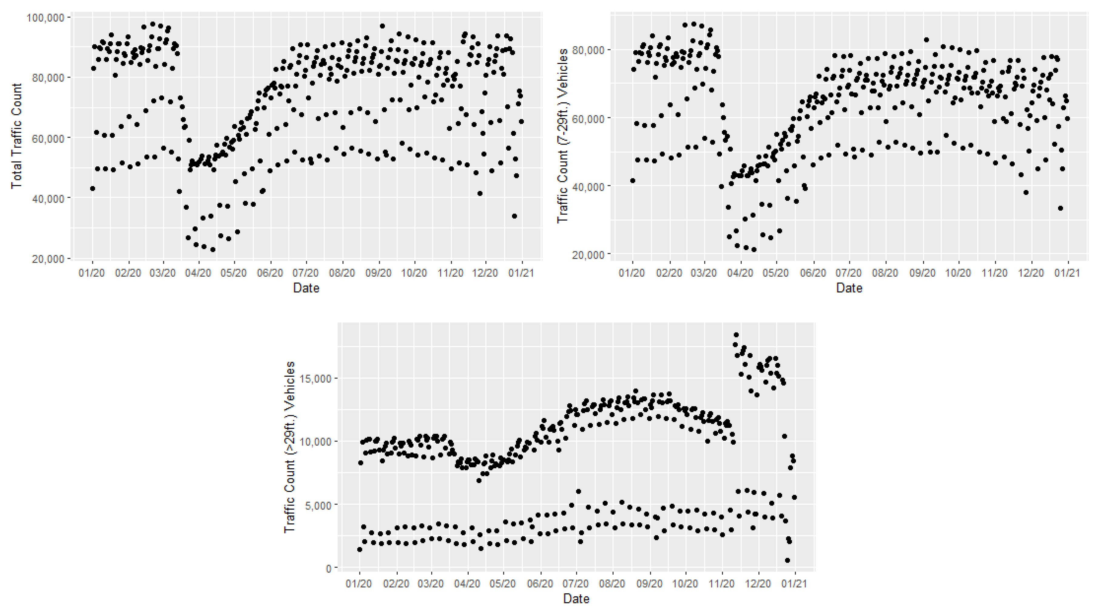
At both the Mt. Healthy and the Northgate sites, traffic volumes significantly decreased for all vehicle classifications during Ohio’s stay-at-home order (Figure 2 and Figure 3). The minimum traffic volumes over this time period occurred near 12 March. Around the beginning of July, traffic counts of all classifications returned to near pre-pandemic 2020 volumes, with total traffic and 7–29 ft traffic sustaining these volumes throughout the rest of the year. Vehicles of 29 ft or greater, however, increased in volume during the latter half of the year. The two trends seen in traffic count volumes in the >29 ft traffic plots (Figure 2 and Figure 3) are indicative of traffic count variation occurring between weekdays and weekends (Figures S2–S4). Traffic volumes of vehicles 0–7 ft in length remained relatively consistent during 2020 while also accounting for less than 1% of total traffic (see Supplementary Materials).

3.2. Predicting Near Road Traffic Counts

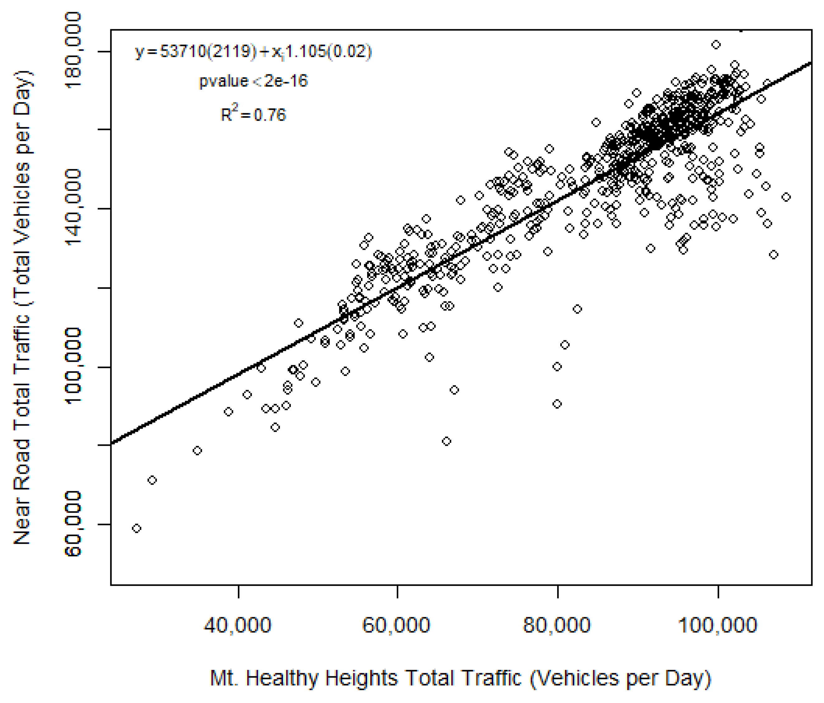
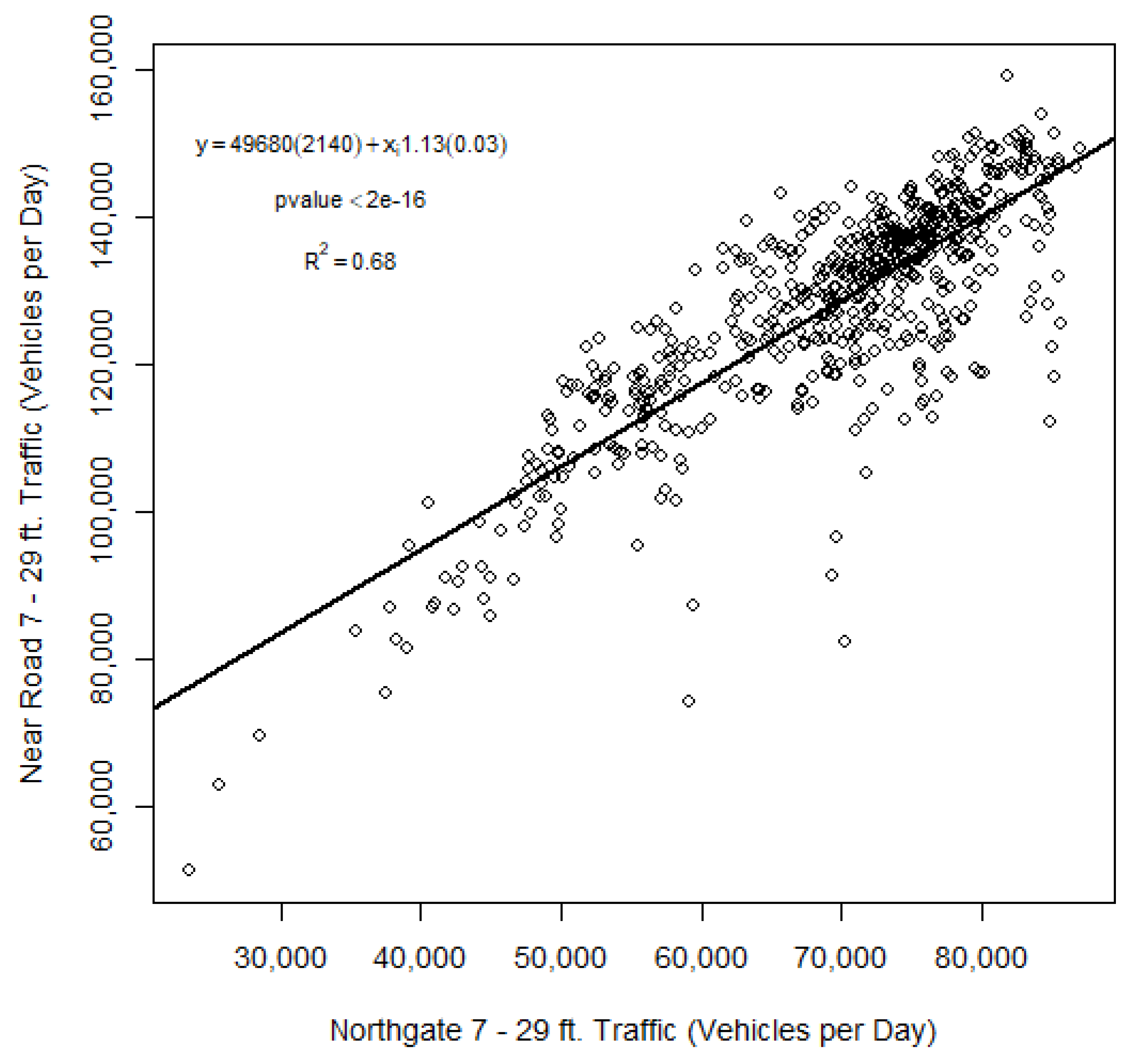
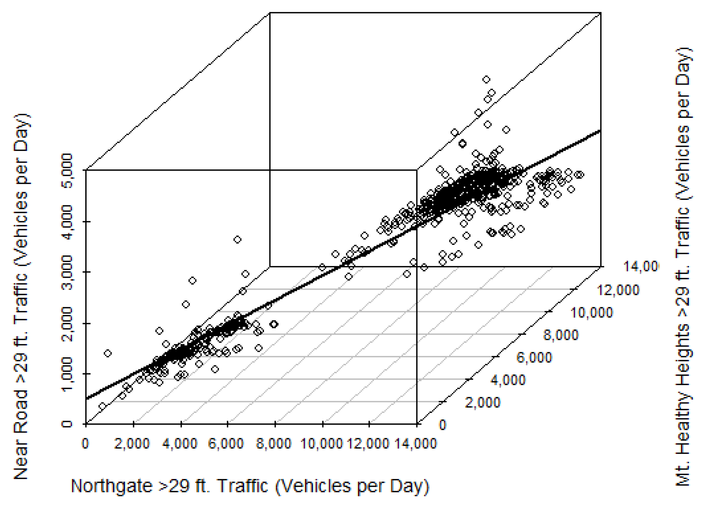
The linear models had R2 values for total traffic counts, 7–29 ft traffic counts, and >29 ft traffic counts of 0.76, 0.69, and 0.72 respectively (Figure 4, Figure 5 and Figure 6). However, for the three vehicle classification types (total traffic, 0–7 ft, and 7–29 ft), traffic volumes from one of either the Mt. Healthy site or the Northgate site were not statistically significant predictors. In these cases, data from the site which was not statistically significant was removed from the regression analysis. Intercept terms which were not statistically significant were also removed in the updated regression analysis.

3.3. 2020 Traffic Trends

During 2020, it was predicted that 7–29 ft traffic made up approximately 85.24% of total traffic, while >29 ft traffic accounted for 14.67% of total traffic (with the remainder being 0–7 ft traffic). Traffic counts of all sizes of vehicles before the onset of the COVID-19 pandemic was predicted to average 139,481 vehicles per day from 1 January through 22 March. As social distancing policies were mandated in Ohio, followed by the closure of schools, restaurants, salons, etc., there was a significant decrease in traffic on Cincinnati roads. Total traffic counts decreased up to 25.55% and did return to near pre-pandemic total traffic levels until around 1 July. Traffic counts for vehicles 7–29 ft in length decreased similarly.
Traffic counts of vehicles >29 ft in length slightly decreased during Ohio’s stay-at-home order by 7.20% compared to pre-pandemic 2020 traffic levels. However, from 1 July through the end of the year, traffic volumes for this vehicle classification increased by 25.95% compared to pre-pandemic 2020. For all time periods, traffic volumes of vehicles >29 ft were higher on weekdays compared to weekends (Figure 7). This is consistent with traffic volume data measured in 2018 at the Near Road site (Figure S4), suggesting that the COVID-19 pandemic policies did not impact relative differences in weekday vs. weekend traffic volumes.

3.4. Intraannual and Interannual Variability of Air Pollutants (PM2.5, BC, CO, NOX, NO2, O3)

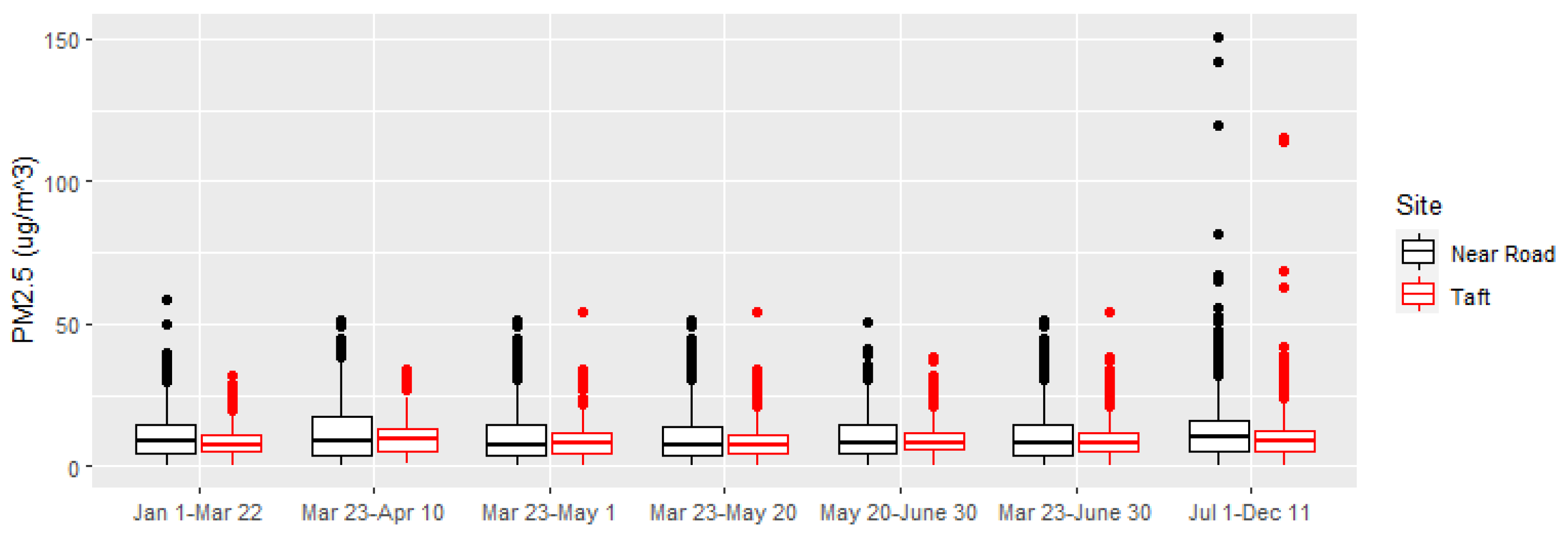
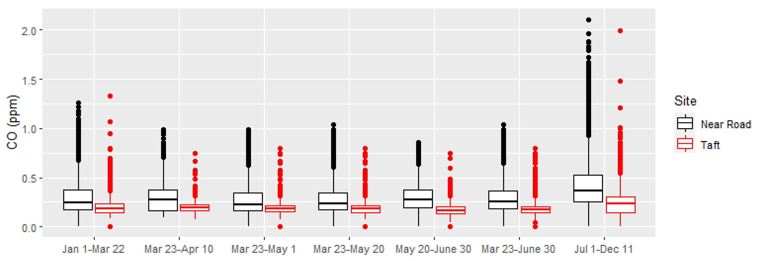
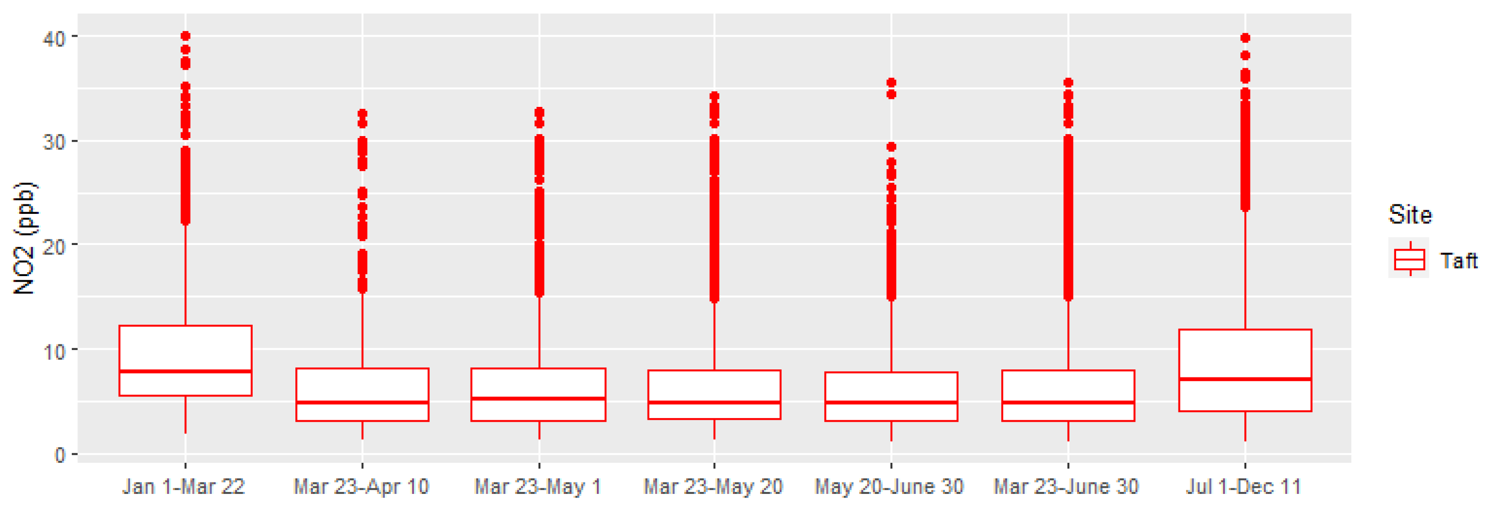
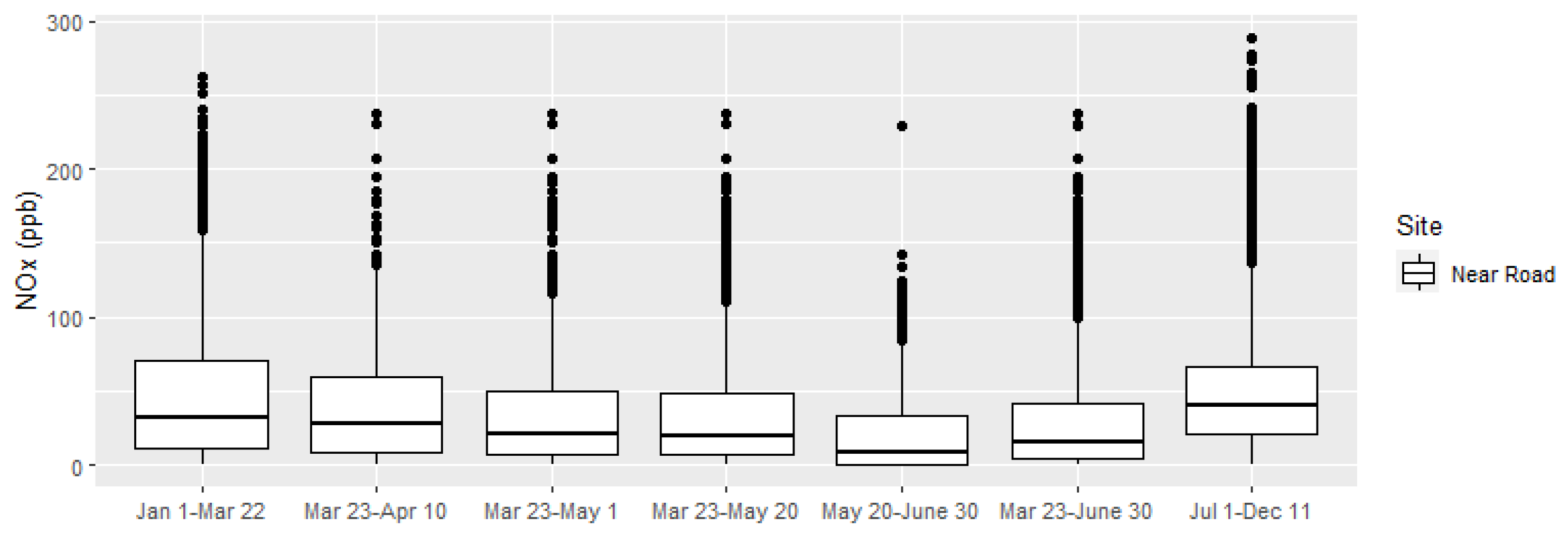
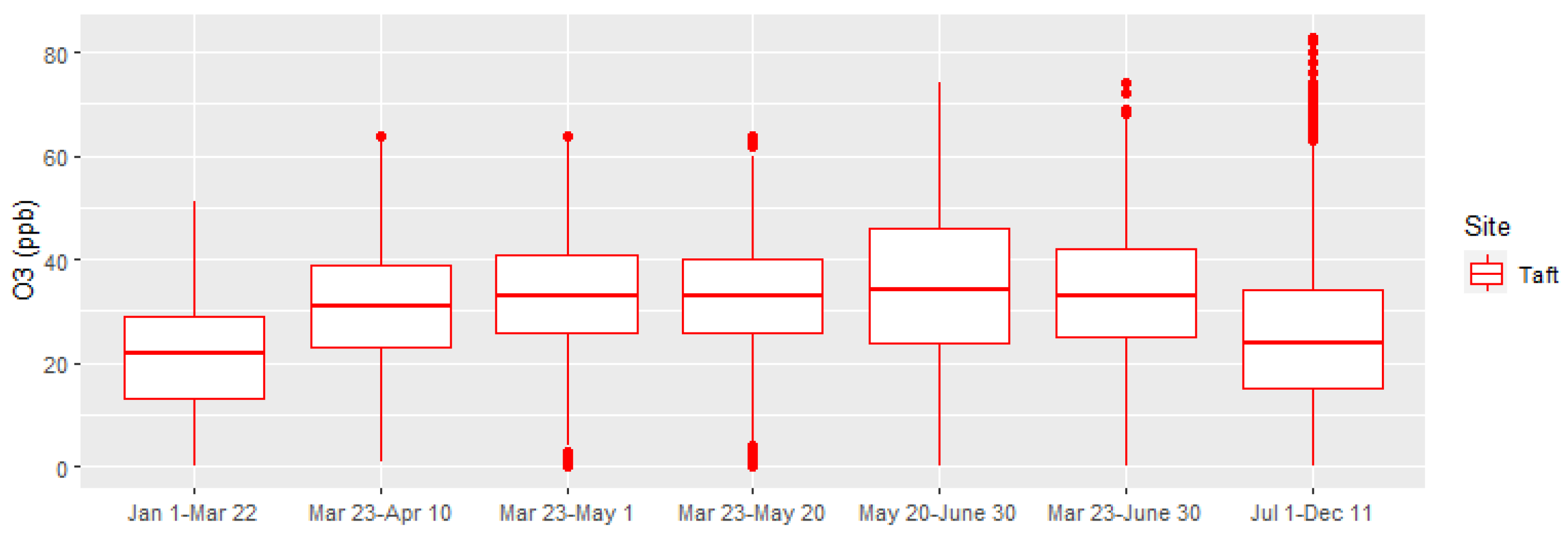
Qualitative evaluation of boxplots show that differences in pollutant concentrations in 2020 at both sites were more pronounced for BC and CO than for PM2.5 and NO2/NOX (Figure 8, Figure 9, Figure 10, Figure 11 and Figure 12). NOX concentrations were much higher at the Near Road site compared to NO2 at the Taft site (Figure 11 and Figure 12). Ozone, measured only at the Taft site, exhibited expected seasonal patterns with highest concentrations in the summer (Figure 13).

3.4.1. PM2.5

PM2.5 levels during the first half of Ohio’s stay-at-home order (23 March–10 April) were significantly higher than those pre-pandemic 2020 at both Taft (23.51%, p-value << 0.001, Table S12) and Near Road (15.69%, p-value << 0.001, Table S10) (Figure 14). PM2.5 levels during this time were also higher than those during every time period of interest of 2020 (aside from 1 July–11 December) and significantly higher than historical levels (2016–2018) at Taft. These elevated ambient PM2.5 concentrations were unexpected since total traffic counts during this time period were 24.41% lower than pre-pandemic 2020 total traffic counts (Table S5). On the other hand, traffic volumes of >29 ft vehicles were only 2.49% lower during the first half of the stay-at-home order than pre-pandemic traffic volumes (Table S5). This suggests that the relatively large decrease in volumes of vehicles 7–29 ft did not contribute significantly to a decrease in PM2.5. However, the statistically significant increase in PM2.5 for several time periods investigated at both the Taft and the Near Road sites suggest that other factors, such as meteorology or non-traffic emitters, may have contributed to PM2.5 in the region during this time.
At the Near Road site, PM2.5 concentrations in 2020 were about the same as pre-COVID over each time period analyzed. At the Taft site, PM2.5 increased over these time periods, with a 9.44% increase (p-value = 6.23 × 10⁻⁴, Table S12) over 23 March–1 May and a 9.45% increase (p-value = 9.55 × 10⁻⁶, Table S12) over 23 March–30 June. Compared to each analyzed historical year, PM2.5 was significantly lower in 2020 over each time period of interest.
The increase in >29 ft vehicle traffic in the latter half of the year compared to pre-pandemic 2020 was accompanied by an increase in PM2.5 when also compared to pre-pandemic concentrations at both Taft (14.25%, p-value << 0.001, Table S12) and Near Road (13.67%, p-value << 0.001, Table S10). Despite this observed increase, PM2.5 at the Near road site from 1 July to 11 December was significantly lower than PM2.5 during the same time period 2017 through 2019 (p-value << 0.001 for each case, Table S11). The Taft site also reported significant decreases in PM2.5 when comparing this time period in 2020 to 2018 and 2019 (p-value < 0.001 in both cases, Table S13).

3.4.2. Black Carbon

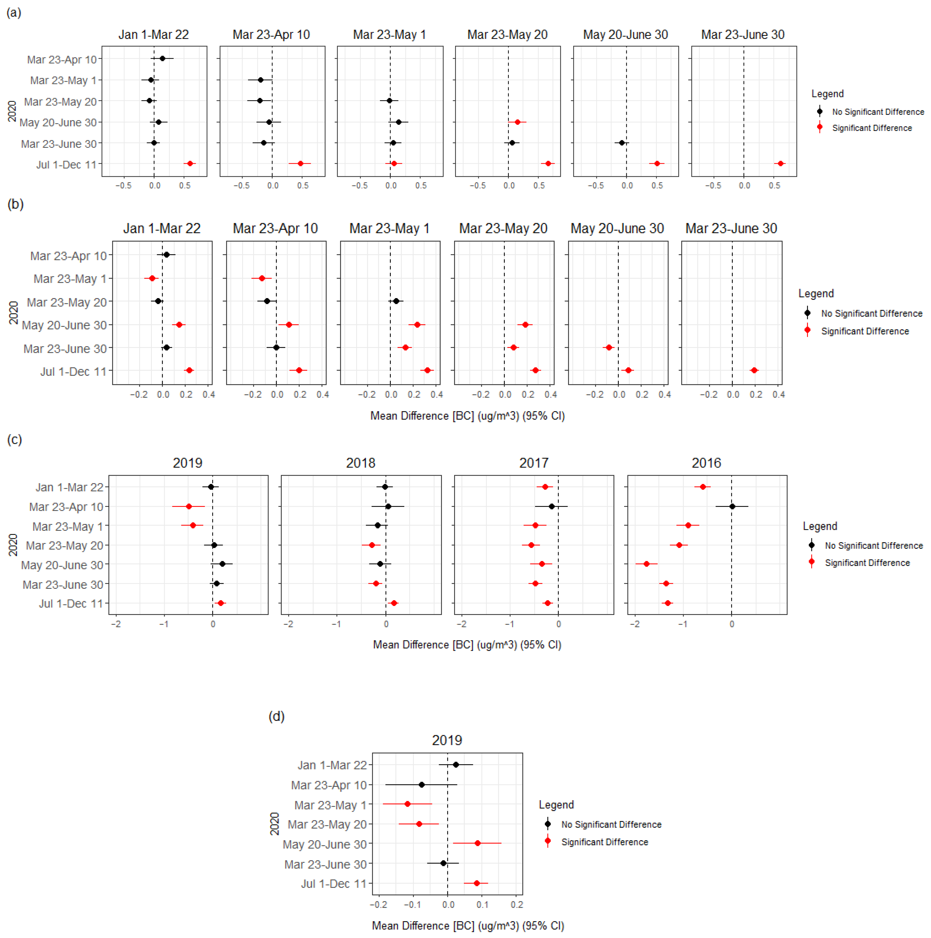
Unlike PM2.5, BC levels during the first half of Ohio’s stay-at-home order (23 March–10 April) were not statistically significantly different as compared to pre-pandemic 2020 at both Taft and Near Road (Figure 15). At Near Road, this trend continued all time periods except from 1 July to 11 December, when BC increased significantly. At Taft, there was a significant decrease in BC over the entirety of Ohio’s stay-at-home order (23 March–1 May) and a statistically significant increase from 20 May to 30 June and from 1 July to 11 December. Similar to PM2.5, BC was higher than pre-pandemic levels from 1 July to 11 December at both Taft (54.76%, p-value << 0.001, Table S16) and Near Road (56.25%, p-value << 0.001, Table S14) and compared to every other time period of interest in 2020.
BC over the latter half of 2020 was significantly higher than BC over this time period in 2018 (Near Road: 11.34%, p-value << 0.001, Table S15) and 2019 (Near Road: 11.24%, p-value << 0.001; Taft: 14.68%, p-value << 0.001, Table S17), but was statistically lower than 2017 (Near Road: 11.60%, p-value << 0.001, Table S17) and 2016 (44.26%, p-value << 0.001, Table S17). The increase in heavy-duty vehicle traffic from 1 July to 11 December (Table S5) is a likely explanation for the increase in BC given that these vehicles tend to use diesel fuel, which is a major source of BC emission [29,30].

3.4.3. CO

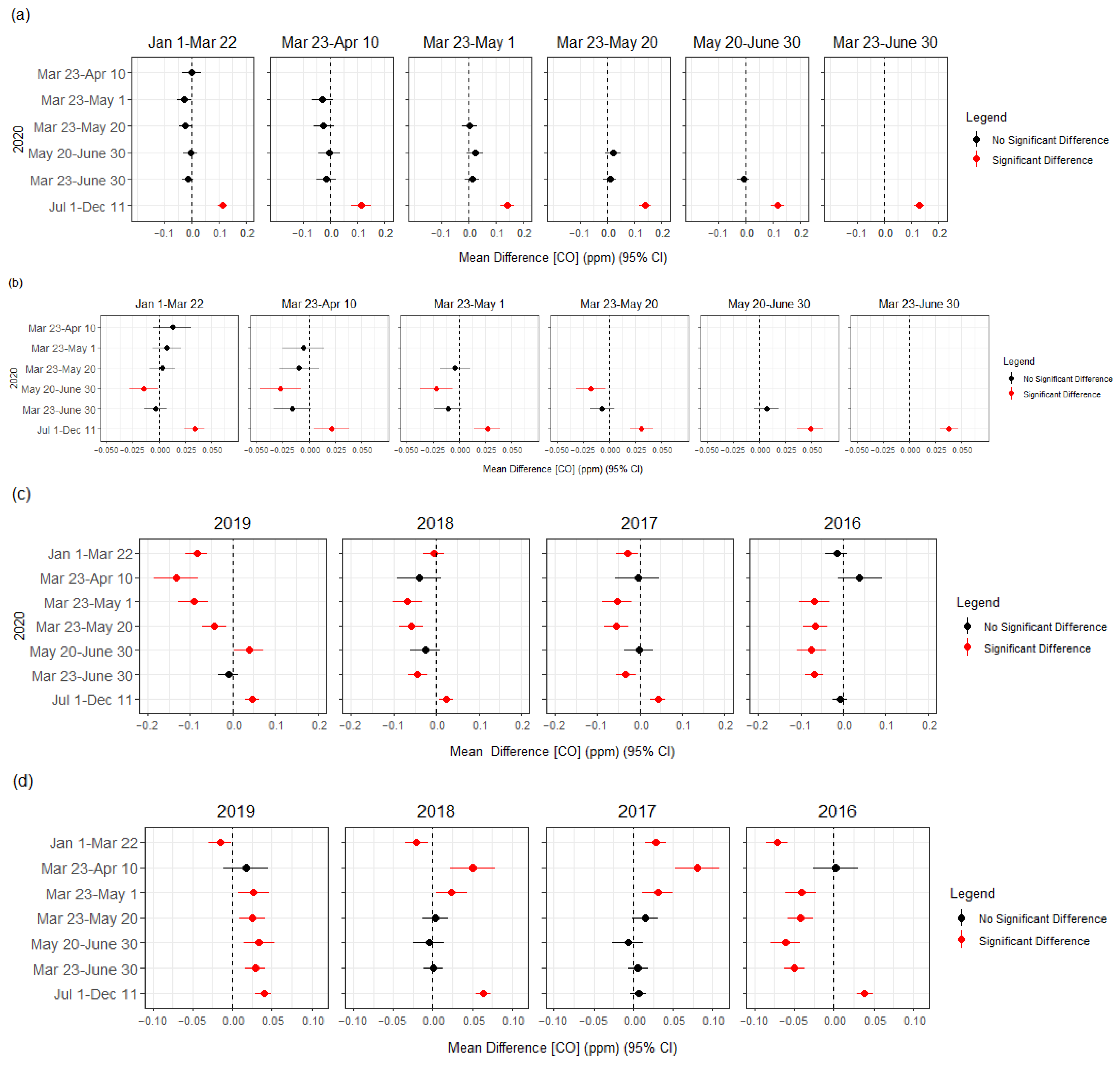
At both the Near Road and the Taft sites, CO concentrations were not statistically significantly different compared to pre-pandemic 2020 for all time periods evaluated except for 1 July–11 December, when CO significantly increased (Figure 16). CO from 1 July to 11 December 2020 was significantly higher than pre-pandemic levels 2020 at Near Road (37%, p-value << 0.001, Table S18) and Taft (18.15%, p-value << 0.001, Table S20). In addition, from 20 May to 30 June at the Taft site, there was a statistically significant decrease in CO when compared to pre-pandemic 2020 (7.66%, p-value << 0.001, Table S20). At this time, total traffic volumes were 4.77% less than less than pre-pandemic 2020 volumes (Table S5). Traffic volume changes do not seem to have influenced this decrease in CO since larger traffic volume decreases occurred during several other time periods of interest where no change in CO occurred. CO during the first half of 2020 at Near Road tended to be lower than or the same as historical levels (aside from 1 July–11 December), while Taft CO was either higher than or the same as 2017–2019 levels.

3.4.4. NOX/NO2

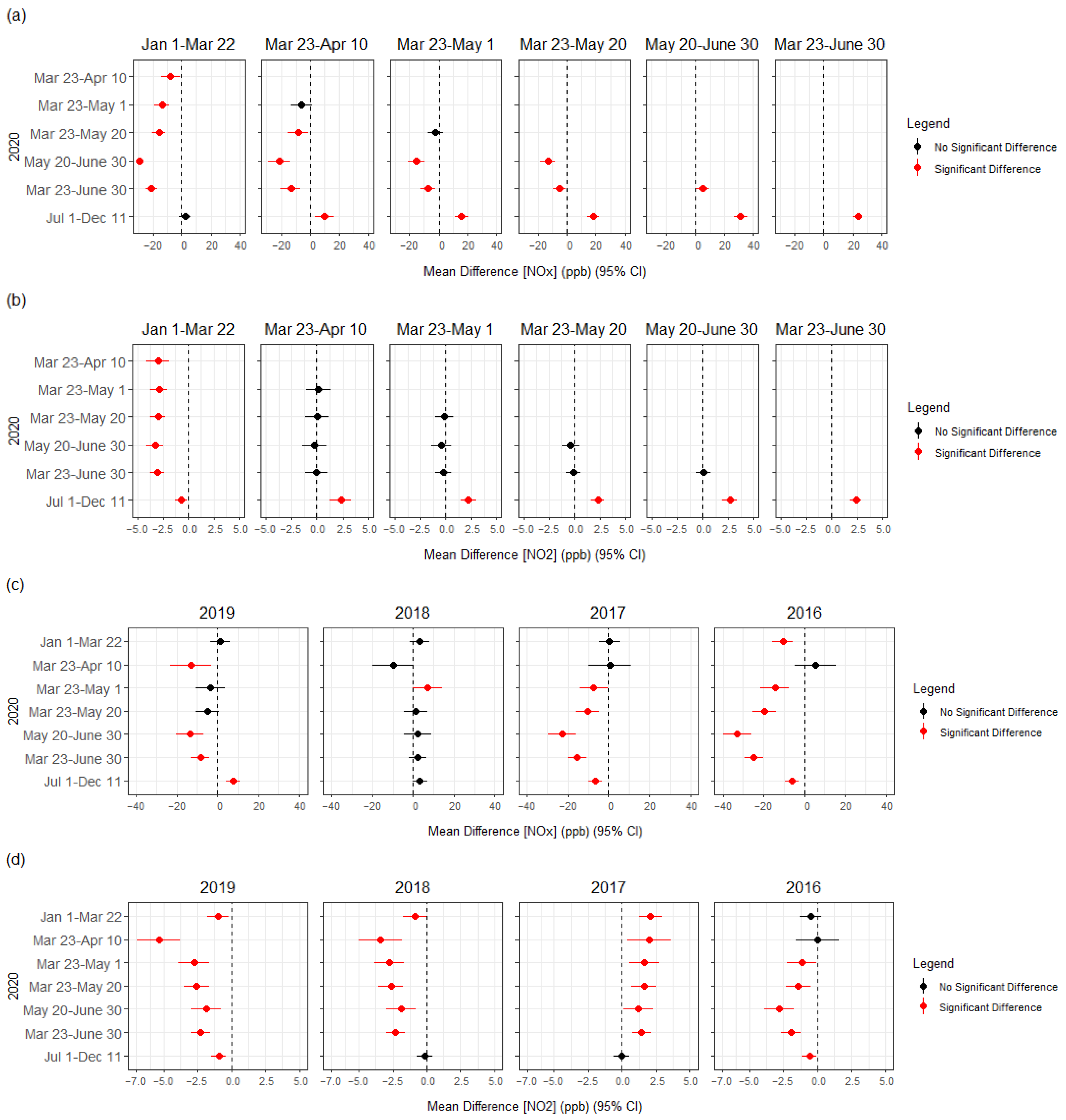
NOX trends followed more expected results compared to BC and PM2.5, as concentrations seemed to more similarly mimic total traffic trends throughout 2020. NOX at the Near Road site decreased significantly into the first half of the year compared to pre-pandemic 2020, with the largest decrease of 60.15% occurring over 20 May–30 June (p-value << 0.001, Table S22) (Figure 17). Over the second half of 2020, NOX concentrations were 4.91% higher (p-value 3.76 × 10⁻²) than pre-COVID levels and were higher than previous years as well (2018 and 2019). NO2 at the Taft site exhibited similar trends to NOX at the Near Road site. Compared to pre-pandemic 2020, NO2 during 2020 was significantly lower over each time period analyzed, with significant decreases ranging from −7.20% to −34.49% (Table S24). NOX during mid-year was significantly lower than previous years (2018 and 2019).

3.4.5. O3

Because O3 is formed through photochemical reactions between NOX and VOCs, O3 concentrations normally peak in the warm summer months when there is increased photochemistry. Due to this inherent seasonality, the intra-annual Tukey tests comparing O3 throughout a single year may not give much insight into changes the COVID-19 pandemic had on Cincinnati’s O3 concentrations. Therefore, Tukey tests were only conducted on interannual data.
Similar to NOX and NO2, reductions in O3 were quite uniform across 2020. Pre-pandemic 2020 O3 was significantly lower than each of the previous four years, with reductions ranging from −14.45% (2016, Table S27) to −22.71% (2018, Table S27) (Figure 18). O3 over every other time period analyzed was also lower in 2020 when compared to historical levels, aside from 20 May–30 June and 23 March–30 June. It has been suggested that Cincinnati is a VOC-sensitive region regarding O3 production [13]. Our results support this when 2020 is compared with 2016, 2017m and 2018 for the time periods 23 March–20 May and 20 May–30 June (Figure 18b). However, when comparing 2020 versus 2019, reductions in NOX did not lead to a statistically significant change in O3 for the time periods 23 March–20 May and 20 May–30 June.

3.5. Meteorological Analysis

During the first half of Ohio’s stay-at-home order (23 March–10 April 2020), PM2.5 at both the Near Road and the Taft sites was significantly higher than pre-COVID 2020 levels. At both sites, BC increased slightly, but this was not statistically significant. There were unexpected significant increases in PM2.5 during the first 2 weeks of Ohio’s stay-at-home order, while there was a concomitant decrease in traffic volumes. As a result, potential meteorological effects, which can impact air quality, were also investigated [31,32].
Descriptive statistics of ambient temperature, relative humidity, pressure, and scalar wind speed (Figures S5–S8, Tables S26–S28) suggest that small changes in these meteorological terms took place when comparing 1 January–22 March to 23 March–10 April (aside from temperature). During this time, average ambient pressure decreased by 0.535%, average wind speed decreased by 5.373%, and average relative humidity decreased by 5.54% (Table S26).
The ABL height was calculated for each day of 2020 at 8 a.m. and 8 p.m. For 1 April–5 April, when pollutant concentrations were especially heigh, the ABL was an average of 520.10 m during the 8 p.m. reading and 551.60 m during the 8 a.m. reading, which were 68.78% and 48.65% lower than the annual average for 2020 (Table 2). During this 5 day time period, PM2.5 at the Near Road and Taft sites was 28.37% and 29.091% higher, respectively, than the annual average for 2020.
The average ABL from 1 July to 11 December was also estimated to be significantly lower than the rest of the year. However, PM2.5 in the 1 July–11 December time period, was lower by 12.64% and 3.02% at the Near Road and Taft site, respectively. In addition, there were elevated concentrations of PM2.5, BC, and CO observed across the monitoring network during this time, suggesting that other meteorological factors and/or increased regional emissions may have impacted air pollutant concentrations during 23 March–10 April [33].

4. Discussion

The results of this work are consistent with several other studies focused on air quality changes in the midwestern United States during the COVID-19 pandemic. For example, PM2.5 increased by 19% at the Taft site during 15 March–25 April 2020 when compared to 25 January–7 March 2020, but this was not statistically significant [25]. However, there was a statistically significant 18% increase in PM10. Furthermore, this study also reported statistically significant increases in PM2.5 concentrations in Indianapolis, Seattle, and Cheyenne. There were increases of PM2.5 in St. Louis, Tulsa, Atlanta, Portland, Cleveland, Kansas City, Grantsville, and Bismarck, but these were not statistically significant. At urban monitoring sites in Chicago, there were no statistically significant reductions in PM2.5, suggesting that heavy-duty long-haul transportation are major contributors to air pollution in this region [23].
No US-based studies were found focusing on BC during the COVID-19 pandemic. However, several studies have been conducted in Europe and Asia. BC emissions were reduced by 23 kt in Europe (20% in Italy, 40% in Germany, 34% in Spain, and 22% in France) during lockdowns compared to the same period in the five previous years [34]. During the second half of January 2020, BC emissions declined 70% in eastern China and 48% in northern China compared to the first half of January 2020. Similar to this study, during the first week of the lockdown in northern China, observed BC rose unexpectedly (29%) even though the BC emissions fell, and it was suggested by the authors that stagnant meteorological conditions were responsible for increased BC during this time [35].
For intra-annual analysis in 2020, CO concentrations remained relatively constant, ostensibly because CO concentrations were low and Cincinnati has met the NAAQS CO standard for many years. However, other work showed statistically significant decreases in CO in 14 out of 21 cities as a result of COVID policies [25]. When compared interannually, CO emissions measurements taken from 70 flights from 2015 to 2020 in Washington, DC, and Baltimore, MD were found to have declined to a greater extent in 2020 (−16%) than compared to the trend observed since 2015 (−4.5%), which was attributable to decreases in traffic during the lockdown [36]. This interannual CO trend at the Near Road site was consistent with Lopez-Coto et al. (2022), but not at the Taft site. This suggests that the decreases in CO compared to historical concentrations were more pronounced in areas with elevated traffic such as interstates.
The significant decreases in NOX and NO2 seen in this work are consistent with other work. Across the United States, NO2 declined by 25.5% with an absolute decrease of 4.8 ppb from 13 March to 8 April compared to 2017 through 2019 [22]. Additionally, all 28 sites analyzed reported decreases in NO2, with reductions ranging from −5% (Cheyenne, WY, USA) to −49% (Las Vegas, NV, USA) when comparing 25 January through 7 March 2020 versus 15 March through 25 April 2020 [25]. NOX was also observed to significantly decrease at multiple monitoring sites in Pittsburgh [24]. While PM2.5 is emitted from a myriad of sources, NOX and NO2 are primarily emitted from the burning of fuel [37], suggesting that changes in traffic may have more of an influence on ambient NOX and NO2 concentrations.
Changes in O3 across the US during COVID-19 stay-at-home orders were not uniform. From March to June, O3 concentrations decreased in rural NOX-limited regions (eastern US), while localized increases in O3 were observed in urban areas that are VOC-limited (western US) [38]. This variation was also noticed when O3 concentrations were compared at 27 N-Core sites in the US (25 January–7 March 2020 versus 15 March–25 April 2020). O3 increased by up to 25% (Salt Lake City, UT, USA) and decreased by up to 15% (Indianapolis, IN, USA) [25]. The reduction in O3 compared to historical years seen in this study is consistent with O3 reductions observed in some eastern US cities studied in other work.
The lack of a reduction in PM2.5, BC, and CO during times of such significant reductions in total traffic could indicate the major influence that particular vehicles have on air quality, such as heavy-duty vehicles and outdated passenger cars/trucks. Therefore, the relatively minimal decrease in >29 ft traffic volumes compared to total traffic volumes could have offset any potential improvements to air quality that may have been observed due to reductions in the mobility of Cincinnatians with passenger vehicles.
Continued operation of outdated passenger cars and pickup trucks could have also played a role in offsetting any potential air quality improvements seen from reduced traffic. While many workers across Cincinnati were able to work from home to avoid unnecessary contact with coworkers, plenty of those deemed “essential” workers had to continue their daily commutes to work. An analysis of 2019 data from the Bureau of Labor Statistics found that essential workers in Ohio earned approximately 21.5% less (30,264 USD) than the average income of the entire state [39]. This suggests that the essential workers that remained on Cincinnati roads during Ohio’s stay-at-home order likely tended to have more outdated and low-cost vehicles. Moreover, it was estimated in a Canadian study that <25% of vehicles contribute to >90% of BC and CO emissions and >70% of particle number emissions of an entire fleet [40], suggesting that the observed reduction in traffic may have comprised vehicles belonging to higher-earning citizens whose vehicles are new and efficient enough to minimally contribute to ambient pollutant concentrations.
It should be noted that there were data gaps for each analyzed pollutant at both sites. Traffic volume data were not available during 2020 at the Near Road site, necessitating a linear regression model to estimate traffic volumes. Additionally, traffic volumes at the Taft site could not be accounted for, as no traffic monitoring sites have ever been operated in this location. In addition, data such as make, model, age and fuel types used by the region’s vehicle fleet are not available and are, therefore, a source of uncertainty. Likewise, precipitation data could not be accessed over the entire time period of interest in this study. Additional meteorological data, as well as information of other regional emitters, could provide further insight into unexpected air quality changes during Ohio’s stay-at-home order.

5. Conclusions

Air pollutant and traffic volume data were analyzed in the city of Cincinnati, OH during 2020 to investigate any possible changes that came about in response to the COVID-19 pandemic. Air pollution data from 2016 to 2020 were used from two monitoring sites, a central site (Taft) and a Near Road site. Traffic volumes at the Near Road site for 2020 were predicted a using linear regression analysis based on traffic data at two nearby sites. Predicted traffic volumes in 2020 at the Near Road site were subsequently used to separate time periods of interest for air quality data analysis. The stay-at-home orders mandated in response to the COVID-19 pandemic reduced total traffic volumes in the Cincinnati region from mid-March to July 2020. The largest reductions in traffic volume (−25%) occurred during the first half of the stay-at-home order. From July through the end of 2020, total traffic volumes returned to near pre-pandemic records, while volumes of vehicles >29 ft increased up to 25%. During 2020, changes in air quality in the Cincinnati region were not uniform compared to pre-pandemic 2020, as well as compared to historical data. Statistically significant increases in PM2.5 occurred at both sites (Near Road: 15.68%; Taft: 23.51%) during the first half of Ohio’s stay-at-home order (23 March–10 April) compared to pre-pandemic 2020. These results were unexpected considering this was a period of time when traffic volumes were at their lowest, as well as when reductions in NOX (−15.88%) and NO2 (−31.39%) were observed. During this time, no changes in CO were observed compared to pre-pandemic 2020 at both sites, but Near Road CO tended to be lower than or the same as historical levels, while Taft CO was either higher than or the same as 2017–2019 levels. O3 decreased or stayed the same compared to historical years over each time period analyzed, with reductions ranging from −14.45% to −22.71%. During the latter half of the year, compared to pre-pandemic 2020, increases in PM2.5 (Near Road: 13.67%; Taft: 14.23%), BC (Near Road: 56.25%; Taft: 54.76%), and CO (Near Road: 37.02%; Taft: 18.15%) were observed. This likely can be explained by the heavy-duty vehicle volume observed during this time. Meteorological analyses of ambient temperature, relative humidity, pressure, and scalar wind speed, as well as atmospheric boundary layer, in this work were inconclusive regarding this unexpected increase in ambient PM2.5. Despite the spike in PM2.5 observed during the first half of the stay-at-home order, the air quality index (AQI) was never greater than 100 during this time. In fact, there were only 7 days in all of 2020 when the AQI was above 100, all of which were attributed to O3 (aside from 4 July, where PM2.5 was the driving pollutant). Results of this work suggest that improvements in air quality improvement from reductions in traffic volumes were limited due to the impacts of heavy-duty vehicles, non-traffic emission sources, and/or meteorology.

Supplementary Materials

The following supporting information can be downloaded at https://www.mdpi.com/article/10.3390/atmos13091459/s1: Figure S1: Traffic counts of vehicles 0–7 ft in length at the Mt. Healthy and Northgate sites; Figure S2. Traffic volume counts for vehicles >29 ft by day of the week during 2020; Figure S3. Predicted traffic counts for each classification at the Near Road site by day of the week over 2020; Figure S4. Traffic volume counts for vehicles >29 ft by day of the week during 2018; Figure S5. Boxplots of ambient temperature at the Near Road site during each time period of interest 2016 through 2020; Figure S6. Boxplots of ambient pressure at the Near Road site during each time period of interest 2016 through 2020; Figure S7. Boxplots of ambient relative humidity at the Near Road site during each time period of interest 2016 through 2020; Figure S8. Boxplots of scalar wind speed at the Near Road site during each time period of interest 2016 through 2020; Table S1. Results of round 2 linear regression for prediction of total traffic counts at Near Road site in 2020. Northgate was used as the sole predictor because, when both Northgate and Mt. Healthy were used as predictors, the Northgate site coefficient was not statistically significant (p-value = 0.3365) while the Mt. Heathy site was somewhat significant (p-value = 0.0553); Table S2. Results of round 2 linear regression for prediction of 0–7 ft traffic counts at Near Road site in 2020. The model was built using both Mt. Healthy and Northgate sites as predictors only showed Mt. Healthy site coefficient to be somewhat significant (p-value = 0.0656), while the Northgate site coefficient was not statistically significant (p-value = 0.7022); Table S3. Results of round 2 linear regression for prediction of 7–29 ft traffic counts at Near Road site in 2020. The model was built using both Mt. Healthy and Northgate sites as predictors only showed the Northgate site coefficient to be somewhat significant (p-value =1.2 × 10⁻⁷), while the Mt. Healthy site coefficient was not statistically significant (p-value = 0.0866); Table S4. Results of round 1 linear regression for prediction of total counts >29 ft at Near Road site in 2020; Table S5. Predicted daily traffic counts at the Near Road site for each classification type (total traffic count, 0–7 ft, 7–29 ft, and >29 ft). Percentages shown indicate percent changes in traffic counts for each classification compared to respective classification type from pr × 10−pandemic 2020 (January 1–March 22); Table S6. Mean and standard deviation of pollutant concentration measured at the Near Road and Taft sites during each time period of interest from 2016 through 2020. The first number in each cell represents the mean, while the number in parentheses represents the standard deviation; Table S7. Median pollutant concentration measured at the Near Road and Taft site during each time period of interest from 2016 through 2020; Table S8. Range of pollutant concentration measured at the Near Road and Taft site during each time period of interest from 2016 through 2020; Table S9. Mean BC to PM2.5 ratio measured at the Near Road and Taft site during each time period of interest from 2016 through 2020; Table S10. Results of interannual t-tests for PM2.5 concentrations over time periods of interest at the Near Road site for each year 2017 through 2020; Table S11. Results of interannual t-tests for PM2.5 concentrations over time periods of interest at the Near Road site for each year 2017 through 2020; Table S12. Results of interannual t-tests for PM2.5 concentrations over time periods of interest at the Taft site for each year 2016 through 2020; Table S13. Results of interannual t-tests for PM2.5 concentrations over time periods of interest at the Taft site for each year 2016 through 2020; Table S14. Results of interannual t-tests for BC concentrations over time periods of interest at the Near Road site for each year 2016 through 2020; Table S15. Results of interannual t-tests for BC concentrations over time periods of interest at the Near Road site for each year 2016 through 2020; Table S16. Results of interannual t-tests for BC concentrations over time periods of interest at the Taft site from 2019 through 2020; Table S17. Results of interannual t-tests for BC concentrations over time periods of interest at the Taft site from 2019 through 2020; Table S18. Results of interannual t-tests for CO concentrations over time periods of interest at the Near Road site for each year 2016 through 2020; Table S19. Results of interannual t-tests for CO concentrations over time periods of interest at the Near Road site for each year 2016 through 2020; Table S20. Results of interannual t-tests for CO concentrations over time periods of interest at the Taft site for each year 2016 through 2020; Table S21. Results of interannual t-tests for CO concentrations over time periods of interest at the Taft site for each year 2016 through 2020; Table S22. Results of interannual t-tests for NOX concentrations over time periods of interest at the Near Road site for each year 2016 through 2020; Table S23. Results of interannual t-tests for NOX concentrations over time periods of interest at the Near Road site for each year 2016 through 2020; Table S24. Results of interannual t-tests for NO2 concentrations over time periods of interest at the Near Road site for each year 2016 through 2020; Table S25. Results of interannual t-tests for NO2 concentrations over time periods of interest at the Near Road site for each year 2016 through 2020; Table S26. Results of interannual t-tests for O3 concentrations over time periods of interest at the Taft site for each year 2016 through 2020; Table S27. Results of interannual t-tests for O3 concentrations over time periods of interest at the Taft site for each year 2016 through 2020; Table S28. Mean and standard deviation of meteorological terms analyzed at the Near Road site during each time period of interest 2016 through 2020; Table S29. Median of meteorological terms analyzed at the Near Road site during each time period of interest 2016 through 2020; Table S30. Median of meteorological terms analyzed at the Near Road site during each time period of interest 2016 through 2020; Table S31. Difference in intra-annual 2020 PM2.5 concentrations (μg/m3), as well as 95% confidence interval of each indicated time period at Near Road; Table S32. Difference in interannual PM2.5 concentrations (μg/m3) 2017–2019 compared to 2020, as well as 95% confidence interval of each indicated time period at Near Road; Table S33. Difference in intra-annual 2020 PM2.5 concentrations (μg/m3), as well as 95% confidence interval of each indicated time period at Taft; Table S34. Difference in interannual PM2.5 concentrations (μg/m3) 2016–2019 compared to 2020, as well as 95% confidence interval of each indicated time period at Taft; Table S35. Difference in intra-annual 2020 BC concentrations (μg/m3), as well as 95% confidence interval of each indicated time period at Near Road; Table S36. Difference in interannual BC concentrations (μg/m3) 2016–2019 compared to 2020, as well as 95% confidence interval of each indicated time period at Near Road; Table S37. Difference in intra-annual 2020 BC concentrations (μg/m3), as well as 95% confidence interval of each indicated time period at Taft; Table S38. Difference in interannual BC concentrations (μg/m3) 2019 compared to 2020, as well as 95% confidence interval of each indicated time period at Taft; Table S39. Difference in intra-annual 2020 CO concentrations (ppm), as well as 95% confidence interval of each indicated time period at Near Road; Table S40. Difference in interannual CO concentrations (ppm) 2016–2019 compared to 2020, as well as 95% confidence interval of each indicated time period at Near Road; Table S41. Difference in intra-annual 2020 CO concentrations (ppm), as well as 95% confidence interval of each indicated time period at Taft; Table S42. Difference in interannual CO concentrations (ppb) 2016–2019 compared to 2020, as well as 95% confidence interval of each indicated time period at Taft; Table S43. Difference in intra-annual 2020 NOX concentrations (ppm), as well as 95% confidence interval of each indicated time period at Near Road; Table S44. Difference in interannual NOX concentrations (ppm) 2016–2019 compared to 2020, as well as 95% confidence interval of each indicated time period at Near Road; Table S45. Difference in intra-annual 2020 NO2 concentrations (ppm), as well as 95% confidence interval of each indicated time period at Taft; Table S46. Difference in interannual NO2 concentrations (ppm) 2016–2019 compared to 2020, as well as 95% confidence interval of each indicated time period at Taft; Table S47. Difference in intra-annual 2020 O3 concentrations (ppm), as well as 95% confidence interval of each indicated time period at Taft; Table S48. Difference in interannual O3 concentrations (ppm) 2016–2019 compared to 2020, as well as 95% confidence interval of each indicated time period at Taft.

Author Contributions

Conceptualization, R.H.T. and S.B.; methodology, R.H.T. and S.B.; software, R.H.T.; data curation, R.H.T.; writing—original draft preparation, R.H.T. and S.B.; writing—review and editing, R.H.T. and S.B.; visualization, R.H.T.; supervision, S.B. All authors read and agreed to the published version of the manuscript.

Funding

Research received no external funding.

Institutional Review Board Statement

No animals or humans were involved in this work.

Informed Consent Statement

Not applicable.

Data Availability Statement

Air pollution and meteorological data were accessed from the Southwest Ohio Air Quality Agency.

Acknowledgments

The authors thank the Southwest Ohio Air Quality Agency for providing air quality data.

Conflicts of Interest

The authors declare no conflict of interest.

References

  1. Pinkerton, K.E.; Green, F.H.; Saiki, C.; Vallyathan, V.; Plopper, C.G.; Gopal, V.; Hung, D.; Bahne, E.B.; Lin, S.S.; Ménache, M.G.; et al. Distribution of Particulate Matter and Tissue Remodeling in the Human Lung. Environ. Health Perspect. 2000, 108, 1063–1069. [Google Scholar] [CrossRef] [PubMed]
  2. Atkinson, R.W.; Ross Anderson, H.; Sunyer, J.; Ayres, J.O.N.; Baccini, M.; Vonk, J.M.; Boumghar, A.; Forastiere, F.; Forsberg, B.; Touloumi, G.; et al. Acute effects of particulate air pollution on respiratory admissions: Results from APHEA 2 project. Air Pollution and Health: A European Approach. Am. J. Respir. Crit. Care Med. 2001, 164, 1860–1866. Available online: https://www.ncbi.nlm.nih.gov/pubmed/11734437 (accessed on 2 February 2022). [CrossRef]
  3. Schwartz, J. Air pollution and hospital admissions for the elderly in Detroit, Michigan. Am. J. Respir. Crit. Care Med. 1994, 150, 648–655. [Google Scholar] [CrossRef] [PubMed]
  4. Schwartz, J. Air Pollution and Blood Markers of Cardiovascular Risk. Environ. Health Perspect. 2001, 109 (Suppl. 3), 405–409. [Google Scholar] [CrossRef] [PubMed]
  5. Kloog, I.; Ridgway, B.; Koutrakis, P.; Coull, B.A.; Schwartz, J.D. Long- and Short-Term Exposure to PM2.5 and Mortality: Using Novel Exposure Models. Epidemiology (Camb. Mass.) 2013, 24, 555–561. [Google Scholar] [CrossRef]
  6. Hu, Z. Spatial analysis of MODIS aerosol optical depth, PM2. 5, and chronic coronary heart disease. Int. J. Health Geogr. 2009, 8, 27. [Google Scholar] [CrossRef] [PubMed]
  7. Watterson, T.L.; Sorensen, J.; Martin, R.; Coulombe, R.A., Jr. Effects of PM2.5 Collected from Cache Valley Utah on Genes Associated with the Inflammatory Response in Human Lung Cells. J. Toxicol. Environ. Health Part A 2007, 70, 1731–1744. [Google Scholar] [CrossRef]
  8. Hu, S.; McDonald, R.; Martuzevicius, D.; Biswas, P.; Grinshpun, S.A.; Kelley, A.; Reponen, T.; Lockey, J.; LeMasters, G. UNMIX modeling of ambient PM2.5 near an interstate highway in cincinnati, OH, USA. Atmos. Environ. 2006, 40, 378–395. [Google Scholar] [CrossRef]
  9. Wojas, B.; Almquist, C. Mass concentrations and metals speciation of PM2.5, PM10, and total suspended solids in Oxford, Ohio and comparison with those from metropolitan sites in the Greater Cincinnati region. Atmos. Environ. 2007, 41, 9064–9078. [Google Scholar] [CrossRef]
  10. Lierl, M.B.; Hornung, R.W. Relationship of outdoor air quality to pediatric asthma exacerbations. Ann. Allergy Asthma Immunol. 2003, 90, 28–33. [Google Scholar] [CrossRef]
  11. Cheng, G.; Smith, A.M.; Levin, L.; Epstein, T.; Ryan, P.H.; LeMasters, G.K.; Khurana Hershey, G.K.; Reponen, T.; Villareal, M.; Lockey, J.; et al. Duration of day care attendance during infancy predicts asthma at the age of seven: The Cincinnati Childhood Allergy and Air Pollution Study. Clin. Exp. Allergy 2014, 44, 1274–1281. [Google Scholar] [CrossRef]
  12. DeFranco, E.; Hall, E.; Hossain, M.; Chen, A.; Haynes, E.N.; Jones, D.; Ren, S.; Lu, L.; Muglia, L. Air Pollution and Stillbirth Risk: Exposure to Airborne Particulate Matter during Pregnancy Is Associated with Fetal Death. PLoS ONE 2015, 10, e0120594. [Google Scholar] [CrossRef]
  13. Torres-Jardón, R.; Keener, T.C. Evaluation of Ozone-Nitrogen Oxides-Volatile Organic Compound Sensitivity of Cincinnati, Ohio. J. Air Waste Manag. Assoc. 2006, 56, 322–333. [Google Scholar] [CrossRef]
  14. Singh, A.; Rajput, P.; Sharma, D.; Sarin, M.M.; Singh, D. Black Carbon and Elemental Carbon from Postharvest Agricultural-Waste Burning Emissions in the Indo-Gangetic Plain. Adv. Meteorol. 2014, 2014, 179301. [Google Scholar] [CrossRef]
  15. Lelieveld, J.; Pozzer, A.; Pöschl, U.; Fnais, M.; Haines, A.; Münzel, T. Loss of life expectancy from air pollution compared to other risk factors: A worldwide perspective. Cardiovasc. Res. 2020, 116, 1910–1917. [Google Scholar] [CrossRef]
  16. Brook, R.D.; Rajagopalan, S.; Pope, C.A., III; Brook, J.R.; Bhatnagar, A.; Diez-Roux, A.V.; Holguin, F.; Hong, Y.; Luepker, R.V.; Mittleman, M.A.; et al. Particulate matter air pollution and cardiovascular disease: An update to the scientific statement from the American Heart Association. Circulation 2010, 121, 2331–2378. [Google Scholar] [CrossRef]
  17. COVID-19 Pandemic in Ohio. 21 May. Available online: https://www.healthpolicyohio.org/coronavirus-covid-19-in-ohio/ (accessed on 9 July 2022).
  18. Zhou, X.; Josey, K.; Kamareddine, L.; Caine, M.C.; Liu, T.; Mickley, L.J.; Cooper, M.; Dominici, F. Excess of COVID-19 cases and deaths due to fine particulate matter exposure during the 2020 wildfires in the United States. Sci. Adv. 2021, 7, eabi8789. [Google Scholar] [CrossRef]
  19. Wu, X.; Nethery, R.C.; Sabath, M.B.; Braun, D.; Dominici, F. Air pollution and COVID-19 mortality in the United States: Strengths and limitations of an ecological regression analysis. Sci. Adv. 2020, 6, eabd4049. [Google Scholar] [CrossRef]
  20. Petroni, M.; Hill, D.; Younes, L.; Barkman, L.; Howard, S.; Howell, I.B.; Mirowsky, J.; Collins, M.B. Hazardous air pollutant exposure as a contributing factor to COVID-19 mortality in the United States. Environ. Res. Lett. 2020, 15, 940. [Google Scholar] [CrossRef]
  21. Pozzer, A.; Dominici, F.; Haines, A.; Witt, C.; Münzel, T.; Lelieveld, J. Regional and global contributions of air pollution to risk of death from COVID-19. Cardiovasc. Res. 2020, 116, 2247–2253. [Google Scholar] [CrossRef]
  22. Berman, J.D.; Ebisu, K. Changes in U.S. air pollution during the COVID-19 pandemic. Sci. Total Environ. 2020, 739, 139864. [Google Scholar] [CrossRef] [PubMed]
  23. Steffeck, A.W.T. Insignificant Impacts of COVID-19 Stay-At-Home Orders on Chicago Air Quality. DePaul Discov. 2021, 10, 2. [Google Scholar]
  24. Lange, C.L.; Smith, V.A.; Kahler, D.M. Pittsburgh Air Pollution Changes During the COVID-19 Lockdown. Environ. Adv. 2022, 7, 100149. [Google Scholar] [CrossRef] [PubMed]
  25. Chen, L.W.A.; Chien, L.C.; Li, Y.; Lin, G. Nonuniform impacts of COVID-19 lockdown on air quality over the United States. Sci. Total Environ. 2020, 745, 141105. [Google Scholar] [CrossRef]
  26. Google. Google Maps Cincinnati. 2022. Available online: https://goo.gl/maps/RdwtEDQXWu1bXAKf6 (accessed on 5 May 2022).
  27. Sørensen, J.H.; Rasmussen, A. Method for Calculation of Atmospheric Boundary-Layer Height used in ETEX Dispersion Modeling. In Proceedings of the Sixth Topical Meeting on Emergency Preparedness and Response, San Francisco, CA, USA, 22–25 April 1997. [Google Scholar]
  28. Seidel, D.J.; Ao, C.O.; Li, K. Estimating climatological planetary boundary layer heights from radiosonde observations: Comparison of methods and uncertainty analysis. J. Geophys. Res. 2010, 115, D16113. [Google Scholar] [CrossRef]
  29. Miguel, A.H.; Kirchstetter, T.W.; Harley, R.A.; Hering, S.V. On-Road Emissions of Particulate Polycyclic Aromatic Hydrocarbons and Black Carbon from Gasoline and Diesel Vehicles. Environ. Sci. Technol. 1998, 32, 450–455. [Google Scholar] [CrossRef]
  30. Hamilton, S.D.; Harley, R.A. High-Resolution Modeling and Apportionment of Diesel-Related Contributions to Black Carbon Concentrations. Environ. Sci. Technol. 2021, 55, 12250–12260. [Google Scholar] [CrossRef]
  31. Elminir, H.K. Dependence of urban air pollutants on meteorology. Sci. Total Environ. 2005, 350, 225–237. [Google Scholar] [CrossRef]
  32. Beaver, S.; Palazoglu, A. Influence of synoptic and mesoscale meteorology on ozone pollution potential for San Joaquin Valley of California. Atmos. Environ. 2009, 43, 1779–1788. [Google Scholar] [CrossRef]
  33. Rachel Tumbleson, R.T.; (University of Cincinnati, Cincinnati, OH, USA); Christina Boss, C.B.; (Southwest Ohio Air Quality Agency, Cincinnati, OH, USA). Personal Communication, 2021.
  34. Evangeliou, N.; Platt, S.M.; Eckhardt, S.; Lund Myhre, C.; Laj, P.; Alados-Arboledas, L.; Backman, J.; Brem, B.T.; Fiebig, M.; Flentje, H.; et al. Changes in black carbon emissions over Europe due to COVID-19 lockdowns. Atmos. Chem. Phys. 2021, 21, 2675–2692. [Google Scholar] [CrossRef]
  35. Jia, M.; Evangeliou, N.; Eckhardt, S.; Huang, X.; Gao, J.; Ding, A.; Stohl, A. Black Carbon Emission Reduction Due to COVID-19 Lockdown in China. Geophys. Res. Lett. 2021, 48, e2021GL093243. [Google Scholar] [CrossRef]
  36. Lopez-Coto, I.; Ren, X.; Karion, A.; McKain, K.; Sweeney, C.; Dickerson, R.R.; McDonald, B.C.; Ahn, D.Y.; Salawitch, R.J.; He, H.; et al. Carbon Monoxide Emissions from the Washington, DC, and Baltimore Metropolitan Area: Recent Trend and COVID-19 Anomaly. Environ. Sci. Technol. 2022, 56, 2172–2180. [Google Scholar] [CrossRef]
  37. Basic Information about NO2. Available online: https://www.epa.gov/no2-pollution/basic-information-about-no2 (accessed on 20 July 2022).
  38. Campbell, P.C.; Tong, D.; Tang, Y.; Baker, B.; Lee, P.; Saylor, R.; Stein, A.; Ma, S.; Lamsal, L.; Qu, Z. Impacts of the COVID-19 economic slowdown on ozone pollution in the U.S. Atmos. Environ. 2021, 264, 118713. [Google Scholar] [CrossRef]
  39. The Average Salary of Essential Workers in 2020. May. Available online: https://www.business.org/finance/accounting/average-salary-of-essential-workers/ (accessed on 4 December 2021).
  40. Wang, J.M.; Jeong, C.H.; Zimmerman, N.; Healy, R.M.; Wang, D.K.; Ke, F.; Evans, G.J. Plume-based analysis of vehicle fleet air pollutant emissions and the contribution from high emitters. Atmos. Meas. Tech. 2015, 8, 3263–3275. [Google Scholar] [CrossRef] [Green Version]
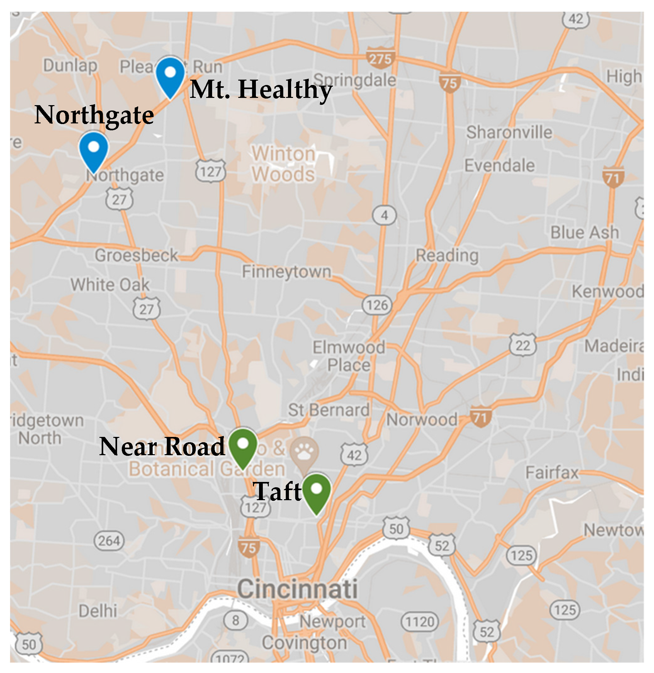
Figure 1. Map of air quality (green) and traffic (blue) monitoring sites used in this study (Google Maps, [26]).
Atmosphere 13 01459 g001
Figure 2. Reported daily average traffic counts at the Northgate site during 2020 for total traffic (top left), 7–29 ft (top right), and >29 ft (bottom center).
Atmosphere 13 01459 g002
Figure 3. Reported daily average traffic counts at the Mt. Healthy site during 2020 for total traffic (top left), 7–29 ft (top right), and >29 ft (bottom center).
Atmosphere 13 01459 g003
Figure 4. Results of using Mt. Healthy total traffic counts to predict Near Road total traffic counts via linear regression. The regression equation, p-value for fit of predictor, and R2 are shown in the top left of the figure.
Atmosphere 13 01459 g004
Figure 5. Results of using Northgate 7–29 ft traffic counts to predict Near Road 7–29 ft traffic counts via linear regression. The regression equation, p-value for fit of predictor, and R2 are shown in the top left of the figure.
Atmosphere 13 01459 g005
Figure 6. Results of using Northgate and Mt. Healthy >29 ft traffic counts to predict Near Road >29 ft traffic counts via linear regression. The regression equation, p-value for fit of predictor, and R2 are shown in the top left of the figure. The two clusters of data seen are representative of weekend vs. weekday traffic volumes (see Figures S2–S4).
Atmosphere 13 01459 g006
Figure 7. Predicted daily traffic counts at the Near Road site for each classification type (total traffic count, 7–29 ft, and >29 ft). The two trends are indicative of traffic volume variation between weekdays and weekends. Note: The increase in vehicles >29 ft in length in mid-November is possibly due to a vehicle accident that occurred on the Brent Spence bridge (I-75 south of the Near Road site) on 11 November 2020. This accident caused the bridge to be closed from 11 November through 22 December forcing traffic to circumvent this widely used means of crossing the Ohio River. I-275 is a means of such navigation; thus, it is hypothesized that the increase in traffic counts seen at the Northgate and Mt. Healthy sites were not accurate predictors of traffic at the Near Road site during this time.
Atmosphere 13 01459 g007
Figure 8. Boxplots of hourly PM2.5 during each time period of interest during 2020 at the Near Road and Taft sites.
Atmosphere 13 01459 g008
Figure 9. Boxplots of hourly BC during each time period of interest during 2020 at the Near Road and Taft sites.
Atmosphere 13 01459 g009
Figure 10. Boxplots of hourly CO during each time period of interest during 2020 at the Near Road and Taft sites.
Atmosphere 13 01459 g010
Figure 11. Boxplots of hourly NO2 during each time period of interest during 2020 at the Taft site.
Atmosphere 13 01459 g011
Figure 12. Boxplots of hourly NOX during each time period of interest during 2020 at the Near Road site.
Atmosphere 13 01459 g012
Figure 13. Boxplots of hourly O3 during each time period of interest during 2020 at the Taft site.
Atmosphere 13 01459 g013
Figure 14. Post hoc test results for intra-annual and interannual PM2.5 comparisons at the Near Road and Taft sites: (a) intra-annual at Near Road; (b) intra-annual at Taft; (c) interannual at Near Road; (d) interannual at Taft. The circles represent the difference in mean hourly PM2.5 concentrations between the two time periods on each axis along with the 95% confidence interval (e.g., top left of top figure: (mean PM2.5 23 March–10 April) − (mean PM2.5 1 January–22 March) = 1.512 ug/m3).
Atmosphere 13 01459 g014aAtmosphere 13 01459 g014b
Figure 15. Post hoc test results for intra-annual and interannual BC concentration comparisons at the Near Road and Taft sites: (a) intra-annual at Near Road; (b) intra-annual at Taft; (c) interannual at Near Road; (d) interannual at Taft. The circles represent the difference in mean hourly BC concentration between the two time periods on each axis along with the 95% confidence interval (e.g., top left of top figure: (mean BC 23 March–10 April) − (mean BC 1 January–22 March) = 0.131 ug/m3).
Atmosphere 13 01459 g015
Figure 16. Post hoc test results for intra-annual and interannual CO concentration comparisons at the Near Road and Taft sites: (a) intra-annual at Near Road; (b) intra-annual at Taft; (c) interannual at Near Road; (d) interannual at Taft. The circles represent the difference in mean hourly CO concentration between the two time periods on each axis along with the 95% confidence interval (e.g., top left of top figure: (mean CO 23 March–10 April) − (mean CO 1 January–22 March) = 0.000255 ppm).
Atmosphere 13 01459 g016
Figure 17. Post hoc test for intra-annual and interannual NOX (Near Road) and NO2 (Taft) concentration comparisons: (a) intra-annual at Near Road; (b) intra-annual at Taft; (c) interannual at Near Road; (d) interannual at Taft. The circles represent the difference in mean NOX concentration between the two time periods on each axis along with the 95% confidence interval (e.g., top left of top figure: (mean NOX 23 March–10 April) − (mean NOX 1 January–22 March) = −7.64 ppb).
Atmosphere 13 01459 g017
Figure 18. Post hoc test results for intra-annual and interannual hourly O3 concentration comparisons at the Taft site: (a) intra-annual at Taft; (b) interannual at Taft. The circles represent the difference in mean hourly O3 concentration between the two time periods on each axis along with the 95% confidence interval (e.g., top left of top figure: (mean O3 23 March–10 April) − (mean O3 1 January–22 March) = 10.56 ppb).
Atmosphere 13 01459 g018
Table 1. Years each pollutant was analyzed. Not all pollutants were analyzed from 2016 through 2020 at both sites due to a lack of data availability.
SitePM2.5BCCONOXNO2O3
Near Road2017–20202016–20202016–20202016–2020--
Taft2016–20202019–20202016–2020-2016–20202016–2020
Table 2. Average ABL(m) over each indicated time period at 8 p.m. and at 8 a.m. in 2020, as well as average and standard deviation of PM2.5 at the Near Road and Taft sites.
Time1 January–22 March23 March–10 April1 April–5 April23 March–1 May23 March–20 May23 March–30 June1 July–11 DecemberYear Average
8 p.m.1585.612478.87520.0962313.222168.0941807.27787.961665.87
8 a.m.1447.7161432.33551.591260.751261.62892.177673.331074.21
Taft
PM2.5
(µg·m−3)
8.16 (4.585)10.079 (6.05)12.76 (8.011)8.931 (5.548)8.489 (5.312)9.426 (5.575)8.931 (5.44)9.322 (6.531)
Near Road
PM2.5
(µg·m−3)
10.29 (7.597)11.82 (9.82)14.82 (12.47)10.19 (8.699)9.90 (8.471)10.40 (8.023)10.17 (8.306)11.62 (8.662)
Publisher’s Note: MDPI stays neutral with regard to jurisdictional claims in published maps and institutional affiliations.