Article

Particulate Matter Forecasting Using Different Deep Neural Network Topologies and Wavelets for Feature Augmentation

by
Stephanie Lima Jorge Galvão
1,
Júnia Cristina Ortiz Matos
1,
Yasmin Kaore Lago Kitagawa
1,2,
Flávio Santos Conterato
1,
Davidson Martins Moreira
1,
Prashant Kumar
2 and
Erick Giovani Sperandio Nascimento
1,2,3,*
1
Computational Modeling Department, SENAI CIMATEC, Av. Orlando Gomes, n. 1845, Salvador 41650-010, Bahia, Brazil
2
Global Centre for Clean Air Research (GCARE), School of Sustainability, Civil and Environmental Engineering, Faculty of Engineering and Physical Sciences, University of Surrey, Guildford GU2 7XH, UK
3
Surrey Institute for People-Centred Artificial Intelligence, School of Computer Science and Electronic Engineering, Faculty of Engineering and Physical Sciences, University of Surrey, Guildford GU2 7XH, UK
*
Author to whom correspondence should be addressed.
Atmosphere 2022, 13(9), 1451; https://doi.org/10.3390/atmos13091451
Submission received: 29 July 2022 / Revised: 23 August 2022 / Accepted: 1 September 2022 / Published: 8 September 2022
(This article belongs to the Special Issue Shipping Emissions and Air Pollution)

Abstract

:
The concern about air pollution in urban areas has substantially increased worldwide. One of its main components, particulate matter (PM) with aerodynamic diameter of ≤2.5 µm (PM2.5), can be inhaled and deposited in deeper regions of the respiratory system, causing adverse effects on human health, which are even more harmful to children. In this sense, the use of deterministic and stochastic models has become a key tool for predicting atmospheric behavior and, thus, providing information for decision makers to adopt preventive actions to mitigate air pollution impacts. However, stochastic models present their own strengths and weaknesses. To overcome some of disadvantages of deterministic models, there has been an increasing interest in the use of deep learning, due to its simpler implementation and its success on multiple tasks, including time series and air quality forecasting. Thus, the objective of the present study is to develop and evaluate the use of four different topologies of deep artificial neural networks (DNNs), analyzing the impact of feature augmentation in the prediction of PM2.5 concentrations by using five levels of discrete wavelet transform (DWT). The following types of deep neural networks were trained and tested on data collected from two living lab stations next to high-traffic roads in Guildford, UK: multi-layer perceptron (MLP), long short-term memory (LSTM), one-dimensional convolutional neural network (1D-CNN) and a hybrid neural network composed of LSTM and 1D-CNN. The performance of each model in making predictions up to twenty-four hours ahead was quantitatively assessed through statistical metrics. The results show that wavelets improved the forecasting results and that discrete wavelet transform is a relevant tool to enhance the performance of DNN topologies, with special emphasis on the hybrid topology that achieved the best results among the applied models.

1. Introduction

The increase in air pollution in urban areas is a concern on a global scale. Such pollution occurs especially due to anthropogenic activities, such as industrialization, the growth of urbanization, automotive vehicles powered by fossil fuels and agricultural burning [1]. According to United Nations, more than half of the world lives in urban regions (around 55%) and this number is increasing, considering some European countries, such as the United Kingdom, with more than 83% of the population living in urban environments, a figure that continues to increase over time. Consequently, humans have been constantly exposed to variety of harmful components from many sources, mainly those from road vehicles, which are the dominant source of ambient air pollutants, such as particulate matter (PM), nitrogen oxide (NOx), carbon monoxide (CO) and volatile organic compounds (VOCs) [2].
Among these pollutants, PM can be highlighted as one of most critical, as it can cause numerous adverse effects on human health, such as asthma attacks, chronic bronchitis, diabetes, cardiovascular disease and lung cancer [3], and it is strongly associated with respiratory diseases in children [2].
PM is an atmospheric pollutant composed of a mixture of solid and liquid particles suspended in the air [2]. These kinds of particles can be directly emitted through anthropogenic or non-anthropogenic activities, and they are classified according to their aerodynamic diameter and their impacts on human health. PM2.5 includes fine particles with a diameter up to 2.5 µm, which can enter the cardiorespiratory systems. The World Health Organization (WHO) estimates that long-term exposure to PM2.5 increases long-term risk of cardiopulmonary mortality by 6% to 13% per 10 µg/m3 of PM2.5 [4]. Furthermore, results from the European project Aphekom indicate that the life expectancy of the most polluted cities could be increased by approximately 20 months if long-term exposure to PM2.5 were reduced to the annual limits established by the WHO [2].
For these reasons, countries have been encouraged to adopt of even more stringent standards and actions to help control and reduce temporal PM concentrations in urban environments [4]. Hence, the construction of models that predict the concentration of this component up to 24 h ahead in densely populated areas with lower computational complexity and cost arises as a key and strategic tool to assist the monitoring process, support control and preventive actions to improve air quality and, consequently, reduce impacts on the health of the population.
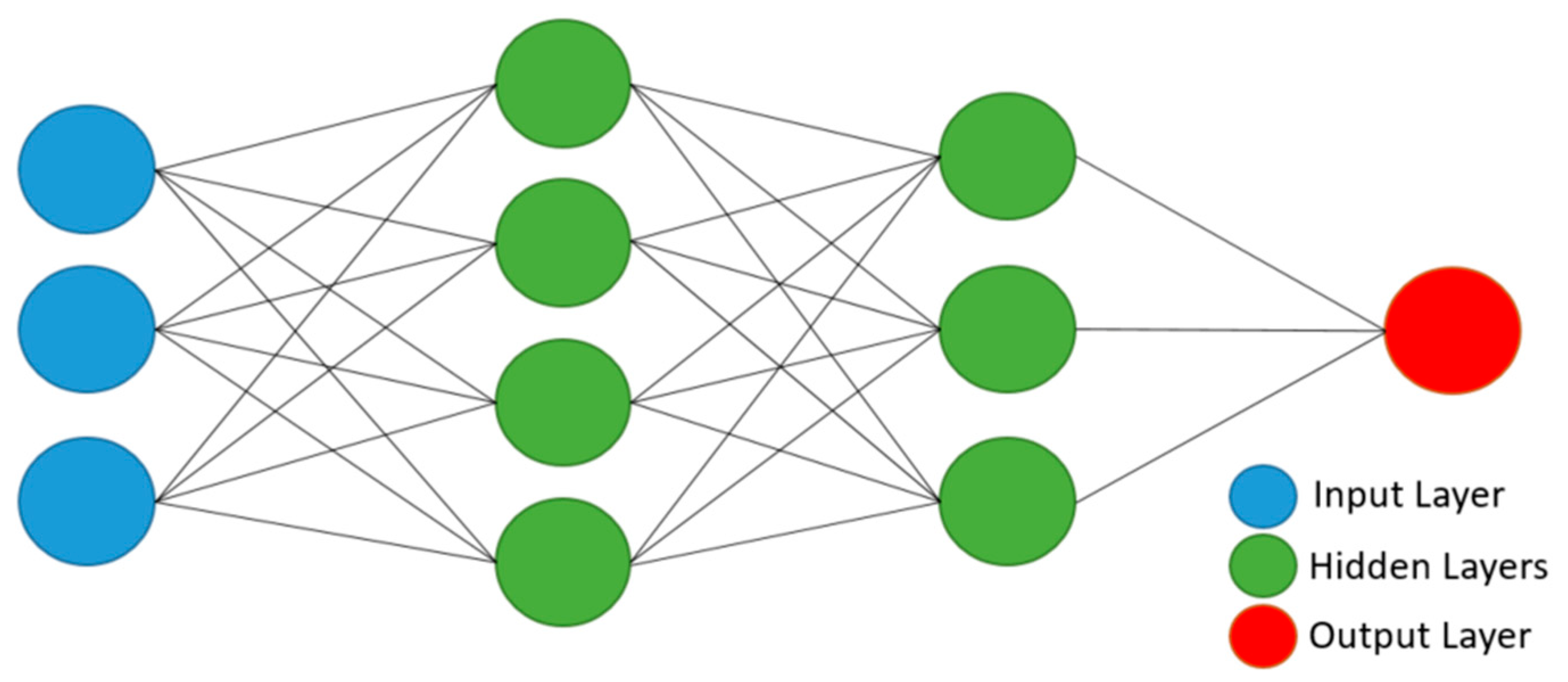
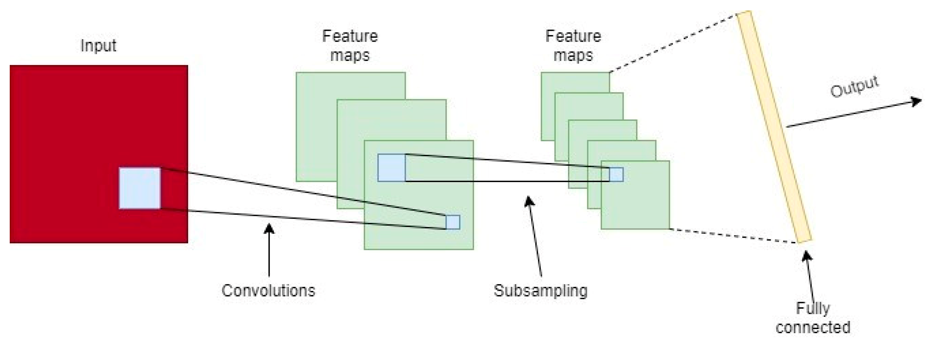
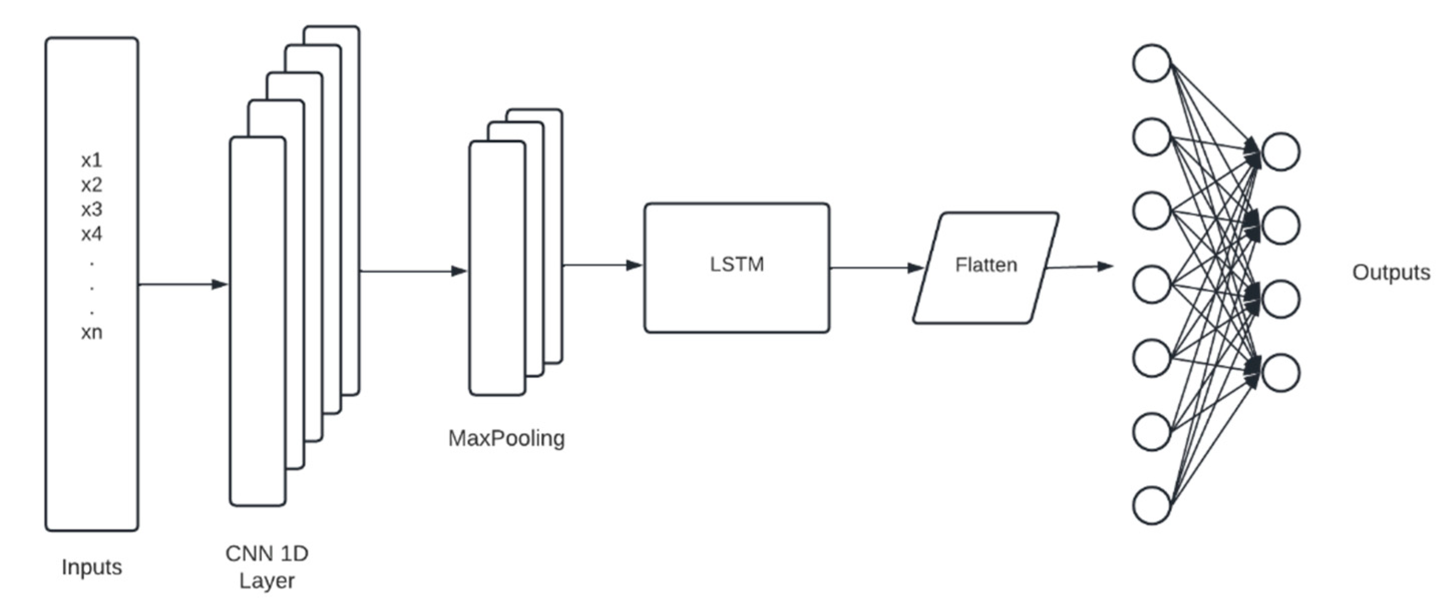
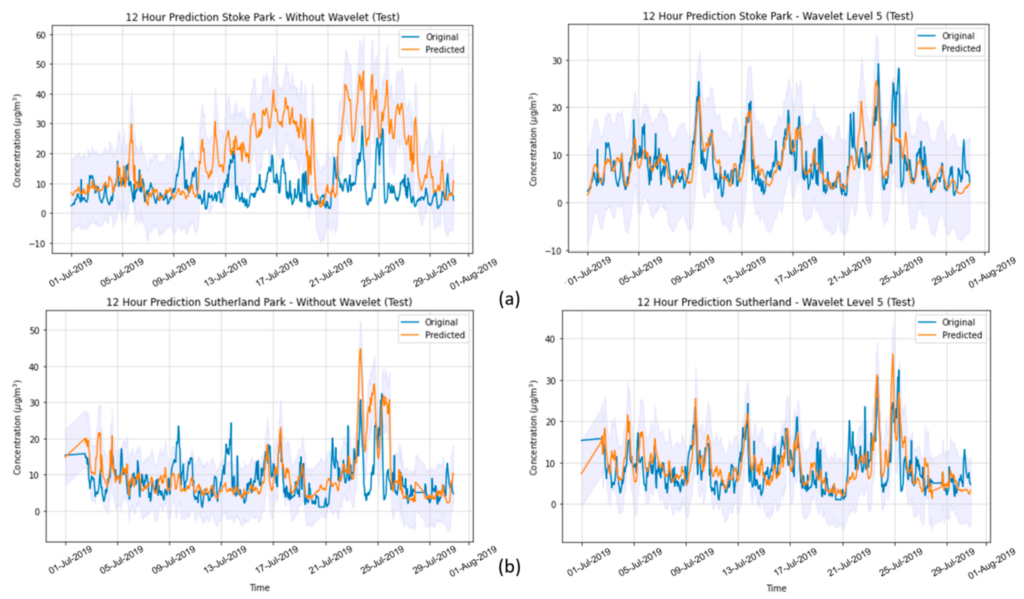
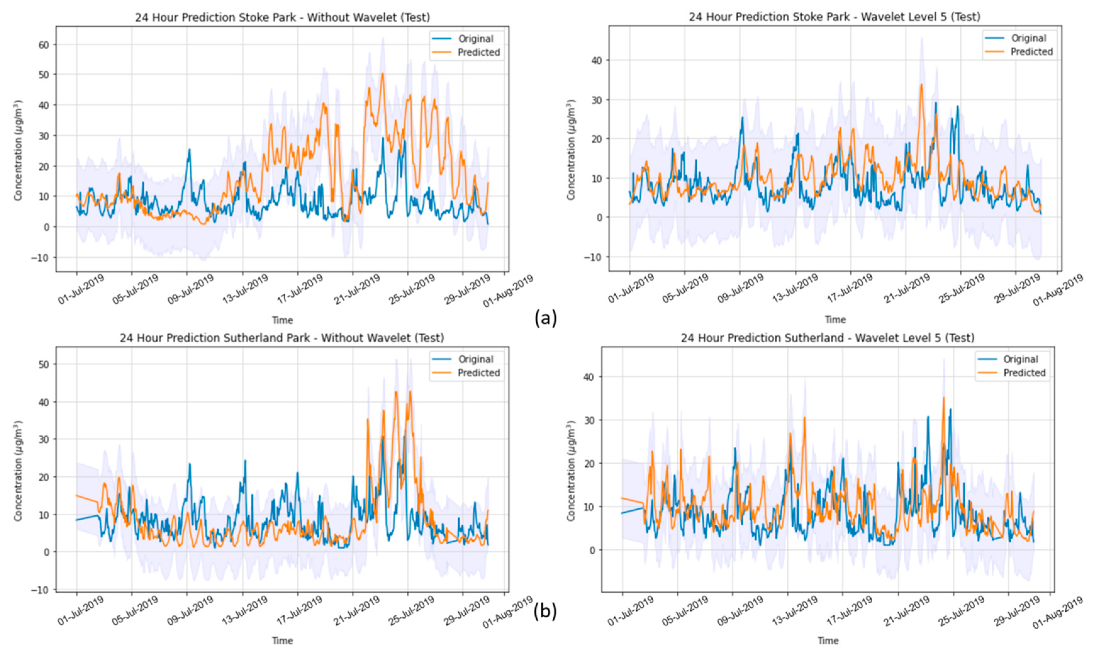
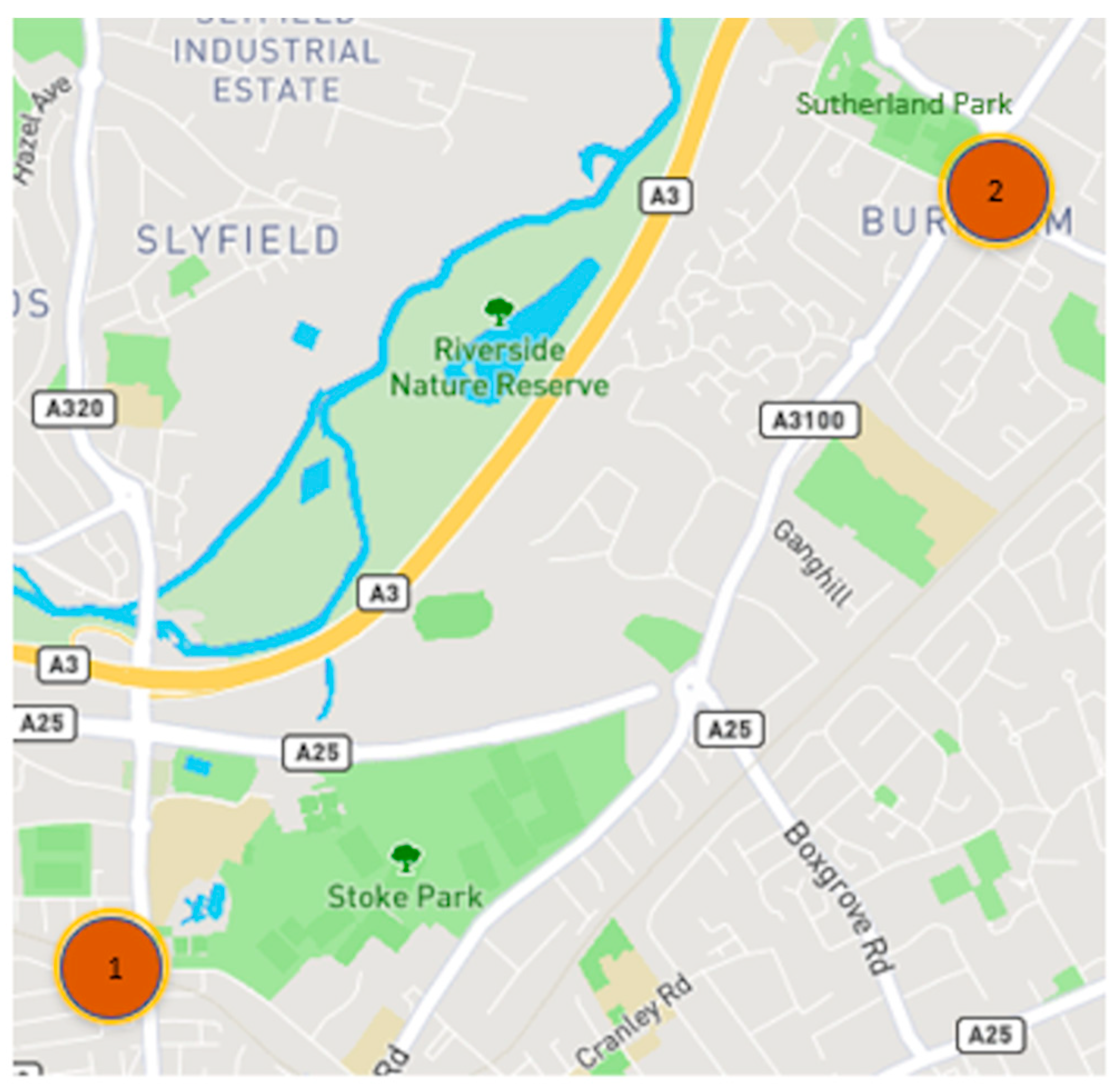
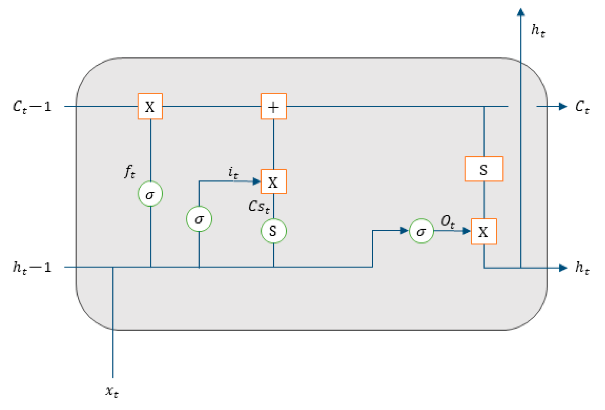
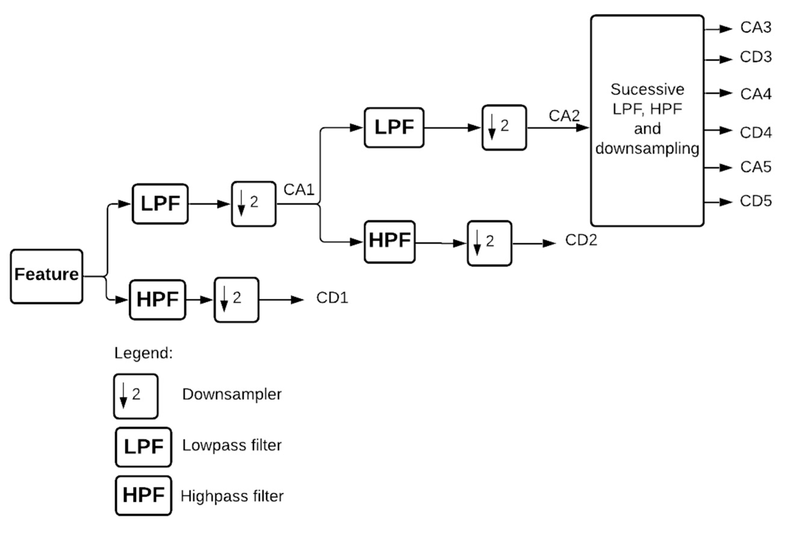
Thus, the objective of this work is to build and evaluate the performance of four deep artificial neural network (DNN) models to predict hourly concentrations of PM2.5 up to 24 h ahead of time, as well as the impact on model performance of applying five-level discrete wavelet transform (DWT) on the data as a feature augmentation method. The DNN types applied were multilayer perceptron (MLP), long short-term memory (LSTM), one-dimensional convolutional neural network (1D-CNN) and a hybrid model (LSTM with 1D-CNN). To train and test the DNN models, data from densely populated areas in Surrey County, UK, characterized by high vehicle traffic were used and augmented by the addition of new features based on the reconstructed detail and approximation signals of wavelet transform from levels 1 to 5. In order to assess the performance of the deep neural networks in the prediction task, all results were compared to a linear regression model as a baseline. Then, they were statistically evaluated according to the following metrics: mean squared error (MSE), mean absolute error (MAE), Pearson’s r and normalized mean squared error (NMSE).
This paper is organized into five sections. In Section 1, we introduce the background and research gaps in the topic areas. In Section 2, we explore the related works in the area of air pollutant forecasting. In Section 3, we present the case study, data, basic concepts of DNN, DWT and additional methods used in this work. In Section 4, we present and discuss the results. Finally, in Section 5, we highlight the main points and present our conclusions, indicating aspects to be explored in future investigations.

2. Related Works

In recent years, several methods have been applied to the task of forecasting air pollution components, mainly using statistical, econometric and deep learning models. Zhang et al. [5] and Badicu et al. [6] assessed the Autoregressive Integrated Moving Average Model (ARIMA), a powerful statistical model, to predict PM concentrations. The former used monthly PM2.5 data from the city Fuzhou, China during the period from August 2014 to July 2016 to train the model and predicted the period of July 2016 to July 2017. The training results presented a mean absolute error (MAE) of 11.4%, with the highest error values in cold seasons, when the real values from PM2.5 were higher than those predicted by the model. The latter worked with data from Bucharest, Romania, considering the period of March to May 2019 with a frequency of 15 min to predict PM10 and PM2.5 concentrations. The results showed that in 89% of cases, the predicted values were under an acceptable limit of uncertainty. However, this kind of approach has some limitations in long-term forecasting, as it uses only past data and it has difficulty reaching high peaks, such as in [5], where it was not able to reach the real peaks of PM2.5.
Considering these limitations, artificial intelligence (AI) methodologies have been used to improve forecasting performance due to their ability to learn from complex nonlinear patterns, their robustness and self-adaptation and their ability to, once correctly trained, perform predictions with limited computational resources and cost when compared to other approaches, such as numerical modeling. Reis Jr. et al. [7] analyzed the use of recurrent neural networks (RNNs) and convolutional neural networks (CNNs) to predict short-term (24 h) ozone concentration. They compared the performance of CNN, recurrent neural network long short-term memory (LSTM) and gated recurrent unit (GRU) structures with a simple multi-layer perceptron (MLP) model. The data were collected between 2001 and 2005 in the region of Vitória in southeastern Brazil. The results showed that the LSTM topology presented an average performance similar to that of MLP but with slightly worse results. However, when considering individual time steps, the LSTM presented the most suitable results for the 9th hour, demonstrating the potential of LSTM for learning long-term behaviors. Ozone forecasting up to 24 h in advance was also evaluated by Alves et al. [8] using the same data but comparing only the MLP model with baseline models: the persistence model and the lasso regression technique. The MLP model proved to be the most effective according to statistical analyses, outperforming the others in almost all forecasting steps, except for the 1st hour.
Regarding PM forecasting, the use of MLP topology to forecast PM particles was investigated by Ahani et al. [9], who compared its performance is with that of the ARIMAX model (ARIMA with exogenous variables) to predict PM2.5 up to 10 h ahead using different feature selection methods. The applied data were from Tehran City, the capital of Iran, and represented a period from 2011 to 2015. The ARIMAX model presented a smaller RMSE in almost all time steps considered, except for the second and the last time steps, for which the MLP presented similar results. This shows that, despite its higher capacity, the single application of artificial neural network (ANN) structures in some data may not outperform simpler methodologies. Thus, it is possible to assess complementary methodologies to make them even more robust. Yang et al. [10] used four different DNN topologies to predict PM2.5 and PM10, including two hybrid models. The DNNs used were GRU, LSTM, CNN-GRU and CNN-LSTM. Data from 2015 to 2018 were used to make predictions 15 days in advance. The results demonstrated that 15-day predictions remained reliable; however, the most accurate forecasts are up to 7 days in advance. The hybrid models outperformed the single models for all stations, and the CNN-LSTM model produced the fewest errors.
Despite the research that has been conducted using ANNs to predict air pollution components, forecasting accuracy depends on the quality of data provided to the model. This means that the results can still be improved by different representations of data, which can reveal hidden patterns, as well as the application of feature augmentation techniques. Therefore, various studied involving preprocessing methods for time series, such as wavelets, have demonstrated the benefits of their application in improving the performance of ANNs in the task of forecasting PM concentrations. For instance, Wang et al. [11] presented the advantages of using hybrid models combining machine learning techniques and wavelet transforms to predict PM2.5 signal. The prediction was performed 1 h ahead by decomposition of PM2.5 data in low- and high-frequency components that capture the trend and noise from the original signal. The temporal resolution of data was the hourly average concentration in the period from 2016 to 2017. The machine learning methods used were a backpropagation neural network (BPNN) and a support vector machine (SVM). The results indicate that hybrid models are more accurate and stable when using wavelets, highlighting their importance in detecting time and frequency behaviors. Bai et al. [12] also used a BPNN model based on wavelet decomposition to forecast air pollutant (PM10, SO2 and NO2) concentrations but with additional information concerning meteorological conditions. The BPNN model was employed to generate wavelet coefficients of the concentrations of air pollutants for the next day, and then the signals were reconstructed to generate the predictions. The forecasting horizon was the mean of the next 24 h. Findings showed that the results of the W-BPNN model were closer to observed data than those of the BPNN model alone, meaning that the multiresolution data provided by wavelets improve the accuracy of air pollutant concentration forecasting.
Qiao et al. [13] used a hybrid stacked autoencoder (SAE) to solve the LSTM vanishing gradient problem and used wavelet transform (WT) to decompose PM2.5 time series into coefficients as the inputs of an ANN structure to predict average PM2.5 1 day ahead. LSTM outputs were used to reconstruct the signal and generate the predictions. The data were from January 2014 to June 2019, and the resulting model outperformed the six other baseline models, with an MAE of approximately 3.0. The baseline models were SAE-BP (SAE back propagation), SAE-ELM (SAE extreme learning machine), SAE-BiLSTM (SAE bidirectional LSTM) and the same machine learning models without SAE (LSTM, BP and ELM (extreme learning machine)). Results showed that SAE-LSTM predictions were the best compared with the other models, satisfactorily solving the vanishing gradient problem.
Huang et al. [14] developed a hybrid CNN-LSTM model to predict the concentrations of PM2.5 one hour ahead using both air pollution and past meteorological data. They compared their solution with other traditional machine learning techniques and found that it achieved the best results for this task. Li et al. [15] developed another hybrid CNN-LSTM deep neural network to predict PM2.5 concentrations for the next day, comparing their proposed model with univariate and multivariate approaches and LSTM architecture, achieving the best results with their approach. Mirzadeh et al. [16] evaluated a traditional machine learning technique called support vector regression (SVR) with WT to predict PM10, PM2.5, SO2, NO2, CO and O3 in Isfahan, Iran, finding that SVR with WT presented better results and lower uncertainty than the other tested models. The same authors [17] conducted a study to evaluate how WT and traditional AI techniques could be combined to improve the prediction of short (few hours) and long-term (daily) concentrations of PM2.5 using an adaptive neuro-fuzzy inference system (ANFIS), SVR and a shallow ANN. Their results showed that WT combined with SVR and ANFIS achieved the best experimental results among the tested models. Liu et al. [18] presented a combined weighted forecasting model (CWFM) for air pollution concentration forecasting using WT, bidirectional (Bi)-LSTM, Bi-GRU and LSTM, along with a weight assignment, and compared the results of the combined approach with each individual model for prediction of NO2 air pollutants. They concluded that the combined approach presented a better performance than each individual model. Jusong et al. [19] developed a hybrid 3D-CNN and Bi-LSTM deep neural network using WT, feature selection and clustering techniques to predict PM2.5 concentrations up to 10h ahead, achieving the best results compared to other techniques. Araujo et al. [20] also evaluated the combination of WT and ANNs to predict air pollution applied to tropospheric O3 forecasting, finding that WT enhanced the ANN’s ability to forecast air pollution concentrations.
Despite previous studies with the aim of predicting PM2.5 using machine/deep learning and WT, in the present study, we aim to innovate by systematically constructing and evaluating four different types of DNN combined with systematic selection and application of five different levels of WT, with the aim of predicting hourly PM2.5 concentrations up to 24 h ahead for a highly urbanized region in the UK. This research can provide new and valuable information with respect to how to effectively apply deep learning and WT for PM2.5 forecasting, improving the ability of regulatory, government or other agencies to adopt preventive or contingency measures to improve air quality and reduce air pollution impacts on human health in urban areas.

3. Materials and Methods

3.1. Case Study and Data Description

As a part of the iSCAPE (Improving the Smart Control of Air Pollution in Europe) project, with the aim of developing integrated strategies to control air pollution in European cities, a diverse set of data was collected (https://www.iscapeproject.eu/iscape-data, accessed on 31 August 2022). One of these approaches consisted of the use of living lab stations (LLSs), which provided environmental and atmospheric data with the aim of monitoring the performance of implemented interventions, such as low boundary walls and green infrastructure in selected cities. Guildford, UK, is one such city, and the data provided by two LLSs were assessed in this work.
Guildford is located in Guildford Borough, one of the most populated areas in Surrey County [21], where 72% of residents rely on cars as their main mode of transportation, leading to an increased air pollution concentrations. The available data were collected by the University of Surrey in two parks: Stoke Park and Sutherland Memorial Park (Figure 1). Data were obtained in open-road conditions, on the outer side of hedges that delimit the two parks. The Stoke Park data were collected from February to September of 2019, whereas Sutherland Memorial Park data were collected from June to October of the same year. Both datasets have a time resolution of one minute. The measurements used were air temperature, air humidity, air pressure, PM2.5, carbon monoxide (CO), nitrogen dioxide (NO2) and ozone (O3). Table 1 presents the description of all available measured variables in the data.

3.2. Artificial Neural Networks

ANNs are composed of a basic structure called neurons. These structures are combined linearly with associated weights, which are assigned with random values at the start of the training, then passed into an activation function that inserts non-linearities capable of modelling complex relationships. Through the relation of the basic components and the activation functions, ANNs can assume different topologies.
The ANNs explored in this paper were MLP, LSTM, CNN and a hybrid model with the aim of improving the results of LSTM and CNN. A brief explanation of each model is presented in this section.

3.2.1. Multi-Layer Perceptron (MLP)

The multi-layer perceptron neural network (MLP) is the simplest artificial neural network topology possible. It is basically a combination of multiple perceptrons, which are the basic neuron units. The functioning of each neuron, or perceptron, can be mathematically expressed by Equation (1).
y x w = f i = 1 m w i x i + b
where yxw is the output of the perceptron, f is the activation function, xi is an attribute or feature from input data vector x of size m, wi represents each weight from weight vector w and b is the bias. In summary, the objective is to determine whether the output of the function (f) triggers (i.e., returns a value other than zero) after summing up the product of the input features and the weights, which are the parameters that are automatically learned through a supervised learning algorithm.
An MLP is generally composed of three or more fully connected layers. Figure 2 presents a schematic diagram of a typical MLP architecture. At least three layers are required: an input layer, a hidden layer and an output layer.
MLPs are suitable for several applications, with their its main parameters represented by the number of layers, the activation functions and the number of neurons in each layer [8], with a flexible topology. The definition of the number of layers and neurons is variable, and the optimal composition is problem-specific. The number of outputs is dependent on specific application requirements, permitting multi-step and multivariate forecasting. The most adequate configuration of these attributes for each of is chosen mostly empirically for each application. All the connections between MLP layers are of the forward kind, which means that backward signal propagation is only possible through a backpropagation algorithm [8]. Although MLPs were not specifically designed to deal with time series forecasting, due to their simplicity and ability to solve complex problems, they have been employed in many studies to predict air pollution components, such as in [5,6,7,8,9,11,22].

3.2.2. Long Short-Term Memory (LSTM)

RNN is a type of neural network created to deal with sequential data distributed across time and space. However, such a structure is prone suffer from the vanishing gradient problem, a characteristic of gradient-based learning methods, which can even prevent neural networks from training. The main difference between RNNs and basic neural networks is that RNNs also establish weighted connections between neurons [13], connected by the hidden state, which carries information from the immediately previous steps and overwrites at every step with no special or selective control of what is memorized or forgotten. This limits the ability of traditional RNNs to correctly represent long-term relationships present in time series or other sequential data.
To tackle this issue, LSTM arose as an alternatives to solve the vanishing gradient problem of conventional RNN topologies. LSTM is a model structured in the form of chains comprising the cell state, input gate, forget gate and output gate, making connections with the next cell through the cell state and hidden state [23]. The cell state is a kind of selective memory of the past, and the gates work interchangeably to control the flow of data in the cell state. The input gate processes the input and decides whether it is relevant to change the memory available in the cell state. The forget gate decides which data should be kept from older output, controlling the flow of the hidden state and deciding which information should be carried to the next cell.
To train an LSTM neural network, the input data need to be three-dimensional because of the addition of the lookback, which represents how many steps back are used to predict the next step or variables. Owing to this capacity, LSTM has the ability to learn temporal relations and improve the forecasting results, representing an interesting tool to deal with time series. Figure 3 shows how an LSTM cell is structured. All lines carry data that can go through pointwise operations, neural network layers, concatenations and replications.
In an LSTM, the cell state acts as an internal selective memory of the past, represented in Figure 3 by the horizontal line starting at ct − 1 and ending at ct. The output of an LSTM cell is represented by h, i.e., the hidden state. The following equations depict the mathematical procedure of an LSTM cell:
f t = σ W f h t 1 , x t + b f
i t = σ W i h t 1 , x t + b i
C s t = S W C h t 1 , x t + b C
C t = f t C t 1 + i t C s
o t = σ W o h t 1 , x t + b o
where f t is the forget gate; i t is the input gate; C s t and C t are the candidates for the cell state and the cell state at timestep t, respectively; o t is the output gate at t; σ is the sigmoid function; S is the a hyperbolic tangent function; W x is the weight matrix of x neurons; h t is the cell output at t; x t is the input at t; and b x is the bias matrix corresponding to x.

3.2.3. Convolutional Neural Networks (CNN)

A CNN is a type of neural network that learns patterns from data through the application of convolutions aimed at learning filters that extract the main features from the data to perform a specific task (see Figure 4). Thus, CNNs are able to learn spatial and temporal relations from data [7]. Consequently, CNNs are able to resize and automatically detect new elements and patterns from data. In addition, pooling layers reduce the size of input sequence, followed by the application of flattening layers, which adjust the shape of data to enter a final regular MLP that concludes the specified task. CNNs are widely applied in image processing [24], and their benefits can be either explored and assessed for time series predictions, for which lookback is also required as an input to the CNN.
The following equations mathematically describe the convolution layer:
G m ,   n = f k m ,   n = j i k j ,   i f m j ,   n i
C l = a l V l
V l = K l · C l 1 + b l
where G is the feature map; f is the input; k , m and n represent the kernel, rows and columns of the result matrix, respectively; the indices j and i are related to the kernel; l is the layer index, V is the intermediate value; K is the tensor that has filters or kernels; C is the result of the convolution; b is the bias; and a is the corresponding activation function. In addition, a pooling layer can be employed to reduce the dimensionality of the size of the output of the convolution step, e.g., by extracting the maximum value (MaxPooling) or the average value (AvgPooling) from the learned and extracted kernels/filters within a fixed-size window, thus decreasing the required processing power for network training.

3.2.4. Hybrid Model

Hybrid models exploit the main functionalities of baseline methods, creating a more robust model that can handle more complex problems. In this sense, the CNN-LSTM method exploits the advantages of CNNs, extracting the most important multidimensional attributes from data, resizing them and sending them as input to the LSTM layers, which can extract more attributes related to temporal relationships. The combination of a CNN and LSTM is expected to deliver more reliable predictions. A representation of such an architecture is shown in Figure 5, with some internal layers that allow for connections between the parts. Thus, this architecture will be evaluated along with others models.

3.3. Wavelet Decomposition for Feature Extraction

WT of a time-domain function is a tool that emerged as an improved version of Fourier transform. Fourier transform consists of taking a time-domain signal and breaking it into a weighted sum of sine and cosine waves to represent it in the frequency domain [25]. However, scientists needed a more appropriate function to represent choppy signals [26], and beyond that, it is necessary to overcome the problem of the window size not changing with frequency [11]. Wavelet analysis can work with different signal temporal resolutions and different basis functions, providing a detailed frequency assessment of all discontinuities and signal patterns, processing data at different scales.
Despite the algebra involved in the process, the discrete wavelet transform (DWT) of a signal is calculated by multiple applications of high-pass and low-pass filters, as shown in Figure 6. The outputs from the former are detail coefficients, and those from the latter are approximation coefficients. The number of times that filters are used is determined by the level of decomposition required. The combination of the two outputs contains the same frequency content as the input signal, but the amount of data is doubled. Therefore, a downsampling procedure is applied to filter outputs, as shown in Figure 6 using a factor of two.
For each feature, there is a specific wavelet family that most satisfactorily represents the original signal in terms of separating more and less significant frequencies. To automate the process of selecting the most suitable wavelet family, Zucatelli et al. [22] proposed a method based on the use of RMSE between the original signal and the reconstructed approximation signal to obtain the most appropriate family for a specific feature. In the present study, this process was applied to all features considered relevant to the analysis.
The importance of WT in machine learning applications lies in the fact that it permits the generation of new features using the approximation and detail coefficients from a pre-determined level of decomposition. The most interesting characteristic of WT is that its individual functions are localized in time and frequency [27], allowing the data to be reconstructed in the same length as the original data, which is relevant to improving ANN model training.

3.4. Model Setup

Before applying data to ANN models, some preprocessing was performed. The available data from the two stations were concatenated to provide more data for the training step. Latitude, longitude and altitude were added to distinguish the regions, and the data were resampled by the average of each hour. Then, five levels of wavelet transform were applied, using the family selection criteria described in [22]. For each feature, five reconstructed detail and approximation signals were obtained.
Previous studies, such as [8], showed the importance of transforming time variables into periodical information by employing trigonometric functions to enable the representation of time cycles, which can lead to improved forecasting performance of DNN models. Thus, the time variable was converted into periodic sine and cosine with the aim of improving the ability of the DNN to learn periodic and temporal relationships [8], depicting them in six new features corresponding to the sine and cosine of hours, days and months according to the following equations:
s i n t a = s i n 2 π t a f
c o s t a = c o s 2 π t a f
where ta is the value of the time attribute being calculated, i.e., hour of the day, day of the month or month of the year; and f is the of possible value of that time attribute in the corresponding time scale, i.e., for hour, the number of hours in a day (24); for day, the number of days in that month; and for month, the number of months in a year (12).
As a result, the final dataset was composed by 86 features, 8 of which were the original features and the remainder of which were the preprocessed and augmented features, as previously described. Finally, all variables were scaled to the same range between zero and one so that they all had the same degree of importance.
Table 2, Table 3, Table 4 and Table 5 present the configurations of each implemented DNN topology. The number of neurons at the input for each DNN is related to the amount of features required as input, i.e., 86, considering all the features generated by the wavelet transforms, as previously explained. In the case of the LSTM, 1D-CNN and the hybrid 1DCNN-LSTM models, a lookback of three samples was set up for training. The output layer of each DNN was set to 24, one for each forecasting hour ahead, totaling 24 h. Therefore, to make predictions once the model was trained, the raw features were collected, as expressed in Table 1, the time series were resampled for hourly frequency, the time attributes were preprocessed as detailed in Equations (10) and (11), the corresponding wavelet transforms and levels were generated, the features between zero and one were scaled and the lookback for each sample was processed (if working with LSTM, 1D-CNN or 1DCNN-LSTM models). As a result, the models output the next 24 h of PM2.5 concentrations, given the input.
The training, validation and test datasets were separated prior to the building, validation and assessment of the models. The training dataset consisted of the concatenation of the Stoke Park data from February to June, in addition to August and September, and the Sutherland Memorial Park dataset corresponding to the months of June, in addition to August to October, both in 2019. From the training dataset, 30% was randomly separated for validation. The month of July 2019 was separated as the test dataset, corresponding to about 15.38% of the total dataset, and was never seen by the models during the training and validation of data from both stations. This was done to assess the final performance of the models in predicting PM2.5 concentrations in order to standardize the tests for the same period for which data were available for both regions.
Table 6 presents the hyperparameters used to train each DNN. No specific hyperparameter search technique was implemented, as the primary target was to evaluate different DNN topologies for the task of forecasting PM2.5 for the next 24 h using WT for feature augmentation. The parameters were set to be practically the same in order to guarantee comparativeness between each topology—except for MLP, which required more 100 epochs than the others models to be successfully trained.

3.5. Model Evaluation

The performance of each DNN topology was quantitatively evaluated using the error metrics mean square error (MSE), mean absolute error (MAE) and normalized mean square error (NMSE), along with the Pearson correlation (r) and coefficient of determination (R2) as correlation metrics, in both training and test datasets according to the following equations:
M S E = 1 n i = 1 n O i F i 2
M A E = 1 n i = 1 n O i F i
N M S E = M S E V a r O
r = i = 1 n O i O ¯ F i F ¯ i = 1 n O i O ¯ 2 i = 1 n F i F ¯ 2
R 2 = 1 i = 1 n O i F i i = 1 n O i O ¯ 2
where n is the number of samples; O i is the i-th observed sample; F i is the corresponding predicted value; O ¯ and F ¯ are the average of all observed and predicted values, respectively; and Var(O) denotes the variance of the O set of observed samples.
In addition, once the models were trained, the prediction intervals for each model and each forecasting horizon were estimated by applying quantile regression to the errors of the predictions made in the validation dataset—which, in this case, was used as the calibration set. To this end, a quantile of q = 0.95 was employed, meaning that the prediction intervals contained a range of values that should include the actual future value with a probability of 95% [28]. The prediction intervals were calculated for each forecast horizon in the test dataset and averaged to generate the final prediction intervals for each model.
After assessing all the prediction results in the test dataset, the model selected as presenting the best metrics was evaluated to determine whether its predictions differed in distribution relative to those of the other model, i.e., whether they were statistically equivalent or not. To this end, the Wilcoxon signed-rank test [29] was employed, as it is a nonparametric statistical technique for comparing two paired or related samples and determining whether their distributions are equal or not. For a given statistical significance (α), if the null hypothesis (H0) can be rejected, i.e., if pα, where p is the calculated p value according to the test; then, the samples are drawn from different distributions. On the contrary, if p > α, H0 cannot be rejected, meaning that the samples are drawn from the same distribution. For this work, α = 0.05 was used.

4. Results and Discussion

4.1. Comparison of Each Approach with and without Wavelet Decomposition

Table 7, Table 8, Table 9 and Table 10 present a comparison of the average metrics of all tested models forecasting 24 h ahead with and without the five wavelet-decomposition levels for both train and test datasets. This average was calculated considering the values of all forecasting hours and stations. The DNN models were compared with a simple linear regression model in order to assess how the DNNs performed in comparison with a baseline approach. Best results in each table for each metric are highlighted in bold.
Table 7 and Table 8 present the metrics for the model results without and with wavelet transforms in the train dataset, respectively. For the train dataset, the hybrid model 1DCNN-LSTM presented the best results for all metrics. The hybrid model achieved the best results with features augmented with wavelets, showing that they were key to increasing the models performance.
Table 9 and Table 10 present the results for metrics of the test dataset, showing that the application of wavelets improved the metrics and, consequently, the results of all topologies, except for MLP, which obtained worse values, except for R2. The hybrid model 1DCNN-LSTM had exhibited the best improvement, with a reduction in MSE of 127.27 to 17.09, representing a reduction of almost 90% in the test dataset. The hybrid architecture with wavelets also presented the best values for all metrics considered, whereas 1D-CNN and LSTM with wavelets demonstrated similar results individually but performed worse than the hybrid 1DCNN-LSTM architecture. Metrics changed from the training to the test metric assessment; in general, the application of wavelet transforms either improved the models’ ability to generalize, as the metrics did not change considerably, presenting with similar metric levels. This highlights the importance of feature augmentation with wavelet transform of time series data to improve the learning ability of DNNs due to their capacity to capture information from the time and frequency domains at the same time and at different scales.
Table 11 and Table 12 present the prediction intervals for each DNN model for all forecasting horizons evaluated in the test dataset without and with wavelets. The smaller the prediction interval, the better because the uncertainties in the predictions are smaller, and the interval is narrower. According to the results, the hybrid model outperformed the others in both cases, presenting the best prediction interval with the 5-level wavelet decomposition.

4.2. Assessing Individual Forecasting Hour Performance for Each Approach

It is also important to verify how each model performs for each forecasting horizon (or each individual hour ahead) in the test dataset, which was never seen by the models during the training and validation. Figure 7 shows the average NMSE and Pearson r behavior metrics for each forecasting hour for each station, considering the data with wavelet transform, as this method was proven to produce superior results relative to no wavelet transform. In general, the hybrid method using 1DCNN-LSTM presented better performance than the others models.
With respect to the NMSE for Stoke Park, the LSTM and MLP models outperformed the 1DCNN-LSTM model for last-hour forecasting, but 1DCNN-LSTM performed better for the overall forecasting hours, with a more consistent and robust performance than that of the other models, including for the Pearson r metric. However, for Sutherland Memorial Park, the MLP model presented the highest errors for the entire range for NMSE, whereas the 1DCNN-LSTM model achieved the best performance in almost all steps, except when LSTM slightly overcame its results for the last forecasting hours. Linear regression and MLP presented the worst performance in Stoke Park for NMSE and Pearson r, whereas MLP presented the worst results for Sutherland Memorial Park data for both metrics, followed by 1DCNN. For both datasets, the smallest error occurred in the first step, increasing along the forecasting horizon. This behavior occurs due to the decreasing ability of all methods with respect to longer-term forecasting, which reduces the capacity of the trained DNN models to make precise inferences about events in farther in the future. Therefore, the prediction performance decreases as the time horizon increases, making the metrics worse in the 24th hour. This also provides a basis for future research in the field of deep neural networks, with the aim of improving the ability of such models to learn and represent longer-term temporal relationships for multivariate time series forecasting. These results are related to a unique model trained for both stations at once.
Figure 8, Figure 9 and Figure 10 show a qualitative analysis of the forecasting behavior for Stoke and Sutherland parks of the 1st, 12th and 24th hours using the 1DCNN-LSTM model built with and without wavelet transforms, including the prediction intervals of the model—plotted as shadowed regions around the predictions. It is possible to notice the qualitative differences between the observed data and the predictions using the specified model with and without wavelets. In general, the application of wavelets increased the model’s ability to predict PM2.5 concentrations. Wavelets contributed to more smoothed and robust predictions, presenting a behavior closer to the real data, with more precise behavior and less noise, which was not the case without wavelets. This behavior was more evident for Stoke Park than for Sutherland Memorial Park, where the predictions without wavelets preserved some characteristics of the original signal but, in general, performed worse than using wavelets. The results of this analysis are in agreement with the quantitative metrics, reflecting the lower error values for the approach using 1DCNN-LSTM and wavelet transforms.

4.3. Evaluation of the Generalization Ability of the DNN

It is important to evaluate of the generalization ability of the DNN, which is demonstrated by analyzing the evolution of the loss (MSE) value for each epoch during the training and validation procedures, using the portion of the data separated for each purpose. The aim is to evaluate whether the model performs well during training with the same behavior both in the training and validation sets. If the model presents different results of loss along the epochs, it may be suffering some sort of under- or overfitting, depending on the behavior of the loss curve measured at each epoch for each set.
Figure 11 presents a graphical evolution, showing that the model generalizes well, presenting no overfitting or underfitting, as the loss of both training and validation presented the same convergence behavior, and PM2.5 predictions in the test dataset, which had not been seen before by the model, were successfully performed.

4.4. Assessment of the Statistical Difference of the Predictions

As presented in Section 3.5, the Wilcoxon signed-rank test was employed to assess whether the models’ predictions differed in terms of distribution and whether they were statistically similar. Table 13 presents the evaluation of the hybrid 1DCNN-LSTM model relative to other DNN models, both with features augmented with 5-level wavelet transforms. According to the results, the Wilcoxon signed-rank test demonstrated that the predictions of the 1DCNN-LSTM had a different distribution than the other DNN models, as the null hypothesis was rejected for every paired test, demonstrating that the hybrid model’s predictions were statistically different from those of the other models.

5. Conclusions

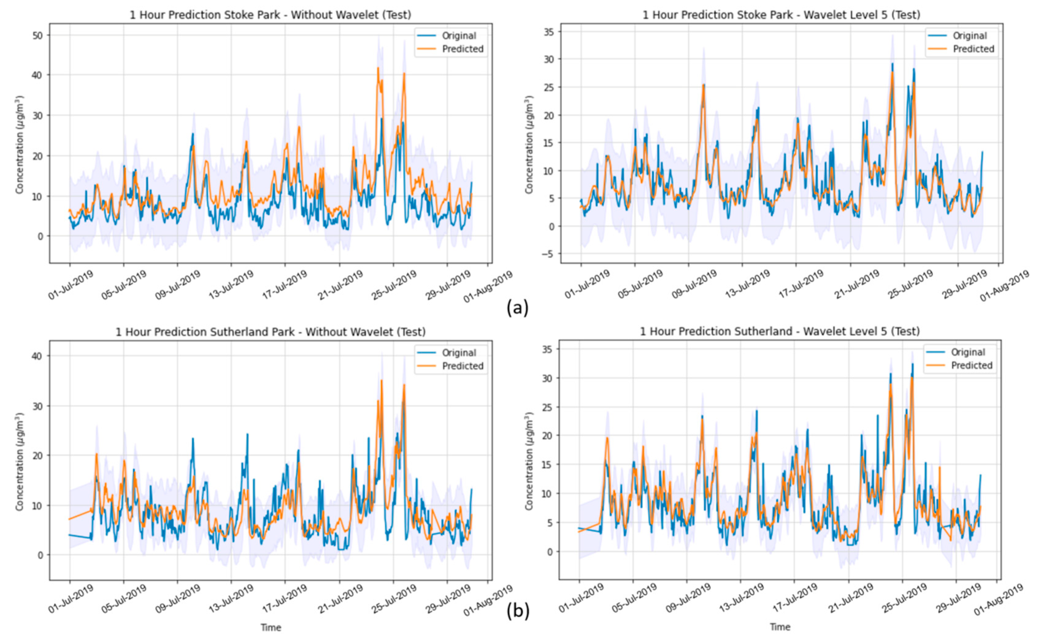
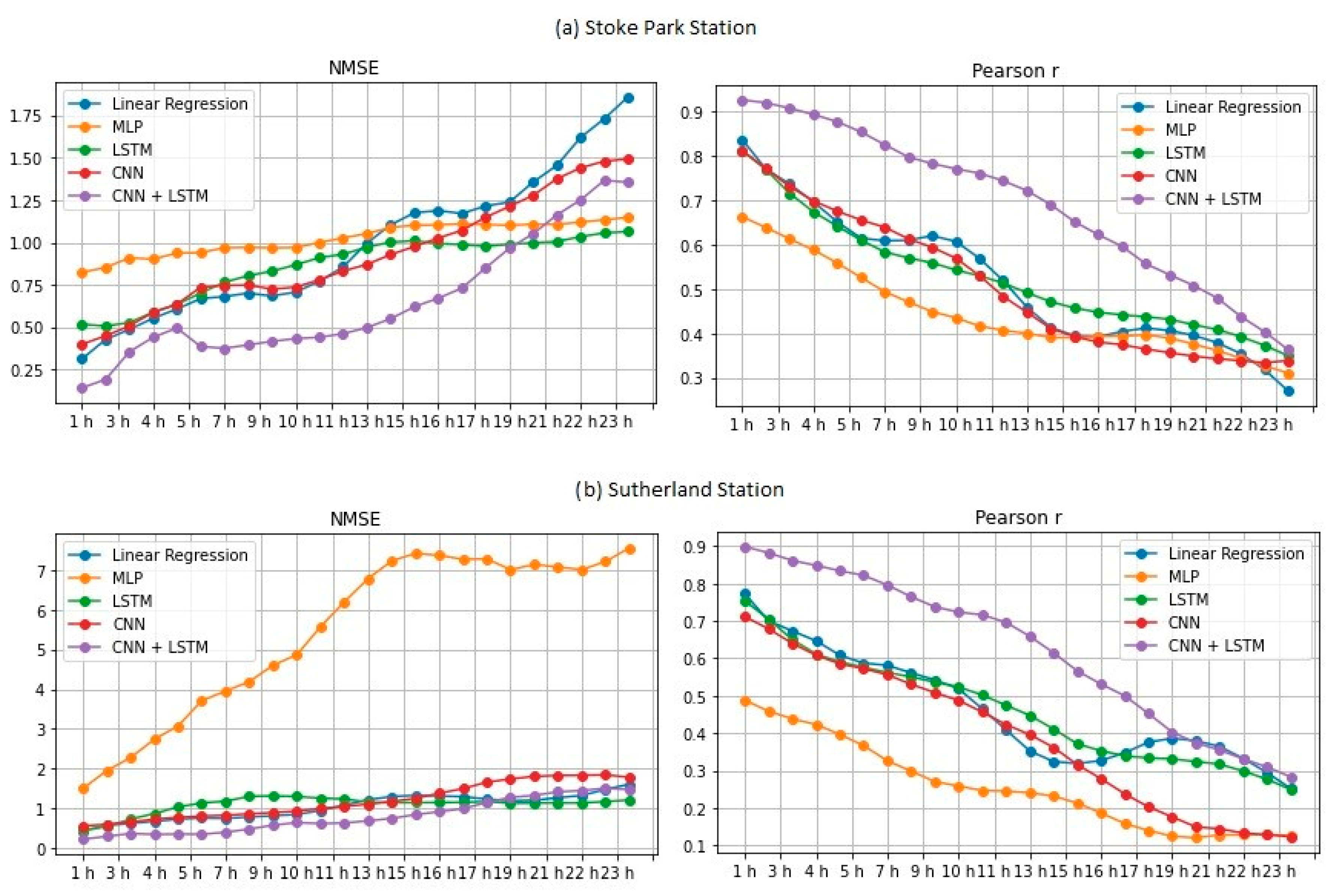
In the present study, we systematically evaluated different deep learning models, along with WT, to predict the concentration of PM2.5 up to 24 h ahead in two open-road regions of Surrey, UK, characterized by the proximity of parks where children and adults perform recreational activities by the high vehicle traffic, which are relevant factors with respect to air pollution monitoring and assessment. The methodology implemented consisted of developing and validating the use of deep learning associated with WT and comparing the results of the tested models with those of simpler methodologies. Different deep neural network topologies were implemented, namely MLP, LSTM, 1D-CNN and 1DCNN-LSTM, with and without WT, along with a linear regressor model as a baseline. The results showed that the best performance was achieved by the 1DCNN-LSTM model among all other DNN architectures, with WT applied on the time series data. The final deep neural network model captured the real data behavior and presented a good generalization of the problem in test data, despite being related to a period of data that was never seen by the model during the training and validation.
WT was implemented with the aim of decomposing the original time-series signals into several low- and high-frequency components, extracting some information from the data that was not yet available. This increased the results of all deep neural networks, which is in line with other previously developed studies [12,13,22]. Our results highlight the positive impact of with respect to improving DNN performance and how this approach is appropriate to deal with complex problems.
Thus, this methodology proved to have a great potential for use in by academics, authorities, industry and society to construct and validate deep learning models to predict hour PM2.5 concentrations in advance for the next 24 h with good performance. This research provides a solid basis for understanding, developing, and evaluating deep learning models for this task, enabling the adoption of preventive or mitigation actions when necessary, such as alerting people to avoid highly polluted areas when the predictions of PM2.5 concentrations reach hazardous levels, avoiding imminent health risks associated with exposure to air pollutants.
In future studies, this methodology can be assessed in other places and scenarios under varying conditions to verify its robustness. Furthermore, other deep neural network approaches and models can be implemented, such as transformers or physics-informed neural networks (PINNs), including feature augmentation methodologies, to assess their capability of predicting long-term PM2.5 concentrations with high fidelity.

Author Contributions

Conceptualization, E.G.S.N. and P.K.; methodology, S.L.J.G. and E.G.S.N.; software, S.L.J.G., J.C.O.M., Y.K.L.K. and F.S.C.; validation, S.L.J.G., E.G.S.N. and D.M.M.; formal analysis, S.L.J.G., J.C.O.M., Y.K.L.K. and E.G.S.N.; investigation, S.L.J.G., D.M.M. and E.G.S.N.; resources, P.K., D.M.M. and E.G.S.N.; data curation, S.L.J.G. and Y.K.L.K.; writing—original draft preparation, S.L.J.G., J.C.O.M., Y.K.L.K. and F.S.C.; writing—review and editing, S.L.J.G., P.K., D.M.M. and E.G.S.N.; visualization, S.L.J.G. and E.G.S.N.; supervision, E.G.S.N.; project administration, E.G.S.N.; funding acquisition, P.K., D.M.M. and E.G.S.N. All authors have read and agreed to the published version of the manuscript.

Funding

This work was partially supported by the Bahia State Research Support Foundation (Fundação de Amparo Pesquisa do Estado da Bahia—FAPESB, Brazil) at SENAI CIMATEC, under project nº CNV 0002/2015. The authors thank the Reference Center on Artificial Intelligence (CRIA) and the Supercomputing Center for Industrial Innovation (CS2i), both from SENAI CIMATEC, as well as the NVIDIA/CIMATEC AI Joint Lab, for infrastructure, technical and scientific support. The authors also thank the iSCAPE (Improving Smart Control of Air Pollution in Europe) project, which was funded by the European Community’s H2020 Programme (H2020-SC5-04-2015) under Grant Agreement No. 689954, as well as the team from the University of Surrey’s Global Centre for Clean Air Research (GCARE), United Kingdom, for providing the data.

Institutional Review Board Statement

Not applicable.

Informed Consent Statement

Not applicable.

Data Availability Statement

The data are publicly available at https://www.iscapeproject.eu/, accessed on 31 August 2022.

Conflicts of Interest

The authors declare no conflict of interest.

References

  1. Doreswamy, K.S.; Harishkumar, K.M.; Gad, I. Forecasting Air Pollution Particulate Matter (PM2.5) Using Machine Learning Regression Models. Procedia Comput. Sci. 2020, 171, 2057–2066. [Google Scholar] [CrossRef]
  2. World Health Organization. Health Effects of Particulate Matter, Policy Implications for Countries in Eastern Europe, Caucasus and Central Asia; World Health Organization. Regional Office for Europe. Available online: https://apps.who.int/iris/handle/10665/344854 (accessed on 31 August 2022).
  3. World Health Organization. Air Pollution, The United Nations. Available online: https://www.who.int/health-topics/air-pollution#tab=tab_2 (accessed on 31 August 2022).
  4. World Health Organization. Occupational and Environmental Health Team, Air Quality Guidelines for Particulate Matter, Ozone, Nitrogen Dioxide, and Sulfur Dioxide: Global Update 2005: Summary of Risk Assessment; World Health Organization: Geneva, Switzerland, 2006. [Google Scholar]
  5. Zhang, L.; Lin, J.; Qiu, R.; Hu, X.; Zhang, H.; Chen, Q.; Tan, H.; Lin, D.; Wang, J. Trend analysis and forecast of PM2.5 in Fuzhou, China using the ARIMA model. Ecol. Indic. 2018, 95, 702–710. [Google Scholar] [CrossRef]
  6. Badicu, A.; Suciu, G.; Balanescu, M.; Dobrea, M.; Birdici, A.; Orza, O.; Pasat, A. PMs concentration forecasting using ARIMA algorithm. In Proceedings of the IEEE 91st Vehicular Technology Conference (VTC2020-Spring), Antwerp, Belgium, 25–28 May 2020. [Google Scholar] [CrossRef]
  7. Reis, A.S., Jr.; Nascimento, E.G.S.; Moreira, D.M. Assessing recurrent and convolutional neural networks for tropospheric ozone forecasting in the region of Vitória, Brazil. WIT Trans. Ecol. Environ. 2020, 244, 101–112. [Google Scholar] [CrossRef]
  8. Alves, L.V.B.; Nascimento, E.G.S.; Moreira, D.M. Hourly tropospheric ozone concentration forecasting using deep learning. WIT Trans. Ecol. Environ. 2019, 236, 129–138. [Google Scholar] [CrossRef]
  9. Ida, K.A.; Majid, S.; Alireza, S. Statistical models for multi-step-ahead forecasting of fine particulate matter in urban areas. Atmos. Pollut. Res. 2019, 10, 689–700. [Google Scholar] [CrossRef]
  10. Yang, G.; Lee, H.; Lee, G. A hybrid deep learning model to forecast particulate matter concentration levels in Seoul, South Korea. Atmosphere 2020, 11, 348. [Google Scholar] [CrossRef]
  11. Wang, P.; Zhang, G.; Chen, F.; He, Y. A hybrid-wavelet model applied for forecasting PM2.5 concentrations in Taiyuan city, China. Atmos. Pollut. Res. 2019, 10, 1884–1894. [Google Scholar] [CrossRef]
  12. Bai, Y.; Li, Y.; Wang, X.; Xie, J.; Li, C. Air pollutants concentrations forecasting using back propagation neural network based on wavelet decomposition with meteorological conditions. Atmos. Pollut. Res. 2016, 7, 557–566. [Google Scholar] [CrossRef]
  13. Qiao, W.; Tian, W.; Tian, Y.; Yang, Q.; Wang, Y.; Zhang, J. The forecasting of PM2.5 using a hybrid model based on wavelet transform and an improved deep learning algorithm. IEEE Access 2019, 7, 142814–142825. [Google Scholar] [CrossRef]
  14. Huang, C.-J.; Kuo, P.-H. A deep cnn-lstm model for particulate matter (PM2.5) forecasting in smart cities. Sensors 2018, 18, 2220. [Google Scholar] [CrossRef]
  15. Li, T.; Hua, M.; Wu, X. A Hybrid CNN-LSTM Model for Forecasting Particulate Matter (PM2.5). IEEE Access 2020, 8, 26933–26940. [Google Scholar] [CrossRef]
  16. Zohre, E.K.; Ruhollah, T.M.; Mohamad, K.; Ali, R.N. Predicting the ground-level pollutants concentrations and identifying the influencing factors using machine learning, wavelet transformation, and remote sensing techniques. Atmos. Pollut. Res. 2021, 12, 101064. [Google Scholar] [CrossRef]
  17. Mirzadeh, S.M.; Nejadkoorki, F.; Mirhoseini, S.A.; Moosavi, V. Developing a wavelet-AI hybrid model for short- and long-term predictions of the pollutant concentration of particulate matter10. Int. J. Environ. Sci. Technol. 2022, 19, 209–222. [Google Scholar] [CrossRef]
  18. Liu, B.; Yu, X.; Chen, J.; Wang, Q. Air pollution concentration forecasting based on wavelet transform and combined weighting forecasting model. Atmos. Pollut. Res. 2021, 12, 101144. [Google Scholar] [CrossRef]
  19. Kim, J.; Wang, X.; Kang, C.; Yu, J.; Li, P. Forecasting air pollutant concentration using a novel spatiotemporal deep learning model based on clustering, feature selection and empirical wavelet transform. Sci. Total Environ. 2021, 801, 149654. [Google Scholar] [CrossRef]
  20. Araujo, M.L.S.; Kitagawa, Y.K.L.; Moreira, D.M.; Nascimento, E.G.S. Forecasting Tropospheric Ozone Using Neural Networks and Wavelets: Case Study of a Tropical Coastal-Urban Area. In Computational Intelligence Methodologies Applied to Sustainable Development Goals; Studies in Computational Intelligence; Verdegay, J.L., Brito, J., Cruz, C., Eds.; Springer: Cham, Switzerland, 2022; Volume 1036. [Google Scholar] [CrossRef]
  21. Abhijith, K.V.; Prashant, K. Field investigations for evaluating green infrastructure effects on air quality in open-road conditions. Atmos. Environ. 2019, 201, 132–147. [Google Scholar] [CrossRef]
  22. Zucatelli, P.J.; Nascimento, E.G.S.; Santos, A.Á.B.; Arce, A.M.G.; Moreira, D.M. An investigation on deep learning and wavelet transform to nowcast wind power and wind power ramp: A case study in Brazil and Uruguay. Energy 2021, 230, 120842. [Google Scholar] [CrossRef]
  23. Le, X.H.; Ho, H.V.; Lee, G.; Jung, S. Application of Long Short-Term Memory (LSTM) neural network for flood forecasting. Water 2019, 11, 1387. [Google Scholar] [CrossRef] [Green Version]
  24. Paolo, A.; Adriano, B.; Maide, B.; Luigi, F. Image processing for medical diagnosis using CNN. Nucl. Instrum. Methods Phys. Res. Sect. A Accel. Spectrometers Detect. Assoc. Equip. 2003, 497, 174–178. [Google Scholar] [CrossRef]
  25. National Instruments. Understanding FFTs and Windowing, Technical Report. Available online: https://www.ni.com/pt-br/innovations/white-papers/06/understanding-ffts-and-windowing.html (accessed on 31 August 2022).
  26. Graps, A. An Introduction to Wavelets. IEEE Comput. Sci. Eng. 1995, 2, 50–61. [Google Scholar] [CrossRef]
  27. Sifuzzaman, M.; Islam, M.R.; Ali, M.Z. Application of Wavelet Transform and its Advantages Compared to Fourier Transform. J. Phys. Sci. 2009, 13, 121–134. [Google Scholar]
  28. Hoshmand, A.R. Business Forecasting: A Practical Approach, 2nd ed.; Routledge: New York, NY, USA, 2010; ISBN 978-1592576128. [Google Scholar]
  29. Corder, G.W.; Foreman, D.I. Nonparametric Statistics for Non-Statisticians: A Step-by-Step Approach, 1st ed.; Wiley: New York, NY, USA, 2009; ISBN 978-0470454619. [Google Scholar]
Figure 1. Location of the monitoring stations, represented as numbers: “1” represents Stoke Park LLS, and “2” represents Sutherland Memorial Park LLS. (Source: https://livinglabs.iscapeproject.eu/, accessed on 31 August 2022).
Atmosphere 13 01451 g001
Figure 2. Schematic diagram representing the basic structure of an MLP architecture. Each circle corresponds to a perceptron.
Atmosphere 13 01451 g002
Figure 3. LSTM cell structure. Arrows, squares and circles represent data flow, pointwise operations and activation functions, respectively.
Atmosphere 13 01451 g003
Figure 4. Typical CNN architecture.
Atmosphere 13 01451 g004
Figure 5. Representation of a CNN-LSTM model considering the inputs, outputs and internal layers.
Atmosphere 13 01451 g005
Figure 6. Illustration of the wavelet decomposition process. LPF, low-pass filter; HPF, high-pass filter. The outputs are downsampled by a factor of two. CA, approximation coefficient; CD, detail coefficient; numbers identify the decomposition level.
Atmosphere 13 01451 g006
Figure 7. Metrics of the hybrid 1DCNN-LSTM model with five-level wavelet decomposition for each forecasting horizon calculated for Stoke Park (a) and Sutherland (b) stations.
Atmosphere 13 01451 g007
Figure 8. Comparison between the predictions of PM2.5 concentrations made with and without wavelets by 1DCNN-LSTM for the 1st hour for (a) Stoke Park Station and (b) Sutherland Memorial Park Station. The shadowed regions represent the prediction intervals of the model.
Atmosphere 13 01451 g008
Figure 9. Comparison between the predictions of PM2.5 concentrations made with and without wavelets by 1DCNN-LSTM for the 12th hour for (a) Stoke Park Station and (b) Sutherland Memorial Park Station. The shadowed regions represent the prediction intervals of the model.
Atmosphere 13 01451 g009
Figure 10. Comparison between the predictions of PM2.5 concentrations made with and without wavelets by 1DCNN-LSTM for the 24th hour for (a) Stoke Park Station and (b) Sutherland Memorial Park Station. The shadowed regions represent the prediction intervals of the model.
Atmosphere 13 01451 g010
Figure 11. Training and validation 1DCNN-LSTM loss graph. “Loss” and “val_loss” represent the evolution of the loss measured at each epoch for the training and validation datasets, respectively.
Atmosphere 13 01451 g011
Table 1. Description of the available measurements in the dataset from both stations.
VariableDescription
TimeTime of the sample, with one-minute frequency
TEMPAir temperature collected at the station
HUMAir humidity collected at the station
PRESSAir pressure collected at the station
PM2.5Concentration of particulate matter with a size ≤2.5 µm
COConcentration of carbon monoxide
NO2Concentration of nitrogen dioxide
O3Concentration of ozone
Table 2. Developed MLP architecture.
LayerLayer TypeNeuronsActivation Function
InputN/A86N/A
First Hidden LayerDense10Sigmoid
Second Hidden LayerDense17ReLu
OutputDense24Sigmoid
Table 3. Developed LSTM architecture.
LayerLayer TypeNeuronsActivation Function
InputN/A86N/A
First Hidden LayerLSTM64Sigmoid
Second Hidden LayerDropout (0.4)N/AN/A
Third Hidden LayerDense12ReLu
OutputDense24Sigmoid
Table 4. Developed 1D-CNN architecture.
LayerLayer TypeNeuronsActivation Function
InputN/A86N/A
First Hidden Layer1D-CNN128Sigmoid
Second Hidden Layer1D-CNN32ReLu
Third Hidden Layer1D-MaxPoolingN/AN/A
Fourth Hidden LayerDropout (0.2)N/AN/A
Fifth Hidden LayerFlattenN/AN/A
Sixth Hidden LayerDense16ReLu
OutputDense24Sigmoid
Table 5. Developed hybrid (1DCNN-LSTM) architecture.
LayerLayer TypeNeuronsActivation Function
InputN/A86N/A
First Hidden Layer1D-CNN128Sigmoid
Second Hidden Layer1D-MaxPoolingN/AN/A
Third Hidden LayerLSTM64Sigmoid
Fourth Hidden LayerDropout (0.2)N/AN/A
Fifth Hidden LayerFlattenN/AN/A
Sixth Hidden LayerDense32ReLu
OutputDense24Sigmoid
Table 6. Hyperparameters used to train each DNN architecture.
LayerMLPLSTM1D-CNN1DCNN-LSTM
OptimizerAdamAdamAdamAdam
Learning Rate0.0010.0010.0010.001
Loss FunctionMSEMSEMSEMSE
Batch Size32323232
Epochs300200200200
Table 7. Average results without wavelets considering both stations in the train dataset.
ModelMSEMAENMSEPearson (r)R2
LR116.307.300.480.740.52
MLP83.855.770.350.800.65
LSTM82.175.740.340.810.66
1D-CNN64.325.530.290.840.71
1DCNN-LSTM12.782.440.080.960.92
Table 8. Average results with five levels of wavelet transform considering both stations in the train dataset.
ModelMSEMAENMSEPearson (r)R2
LR696.5717.951.740.0078−0.74
MLP44.364.480.210.890.79
LSTM35.454.000.320.910.83
1D-CNN27.043.460.130.930.87
1DCNN-LSTM18.642.960.910.960.91
Table 9. Average results without wavelets considering both stations in the test dataset.
ModelMSEMAENMSEPearson (r)R2
LR45.615.381.750.370.47
MLP29.183.931.130.37−0.13
LSTM28.213.861.080.39−0.09
1D-CNN33.274.181.290.37−0.30
1DCNN-LSTM127.277.585.140.40−4.15
Table 10. Average results with five levels of wavelet transform considering both stations in the test dataset.
ModelMSEMAENMSEPearson (r)R2
LR23.753.660.980.52−0.74
MLP84.846.123.150.350.79
LSTM25.103.701.450.490.83
1D-CNN27.193.731.050.450.87
1DCNN-LSTM17.092.970.660.680.91
Table 11. Average prediction intervals for all forecasting horizons for each model in the test dataset without wavelets for both stations.
ModelPrediction Interval (+/−)Mean Prediction Interval Lower BoundMean PredictionMean Prediction Interval Upper Bound
MLP18.23−8.919.3227.55
LSTM18.17−8.779.4027.57
1D-CNN16.23−6.649.5925.82
1DCNN-LSTM9.093.8512.9522.05
Table 12. Average prediction intervals for all forecasting horizons for each model in the test dataset with the five levels of wavelet decomposition for both stations.
ModelPrediction Interval (+/−)Mean Prediction Interval Lower BoundMean PredictionMean Prediction Interval Upper Bound
MLP13.85−2.9110.9424.80
LSTM12.09−3.828.2720.36
1D-CNN10.76−2.658.1118.86
1DCNN-LSTM8.590.218.7917.38
Table 13. Wilcoxon signed-rank test assessment of the predictions of the hybrid 1DCNN-LSTM model against the other models with five-level wavelet transforms. If H0 is rejected, i.e., if pα, α = 0.05, the distributions are different.
ModelStoke
p-Value
Sutherland p-ValueTest Result
MLP0.000.00Different distribution
LSTM0.000.04Different distribution
1D-CNN0.000.00Different distribution
Publisher’s Note: MDPI stays neutral with regard to jurisdictional claims in published maps and institutional affiliations.

