Abstract
The increase in airborne pollution in large cities since the mid-20th century has had a physiologically proven impact on respiratory health, resulting in the irritation and corrosion of the alveolar wall. One of the demographics of the population most affected by this problem is children. This study focuses on the relationship between particulate matter of 2.5 µm (PM2.5) and childhood asthma, which is one of the main respiratory diseases identified in developing countries. The city of Cartagena de Indias, Colombia, is taken as a case study. A relevant correlation between childhood asthma and PM2.5 is found. Incidence series of paediatric asthma on a monthly scale and PM2.5 records in the city of Cartagena are considered. As is common in developing countries, the series was incomplete due to a lack of experts and insufficient economical resources. Therefore, several statistical and analytical processes were applied to provide sufficient quality to the series. An improvement of the time scale of the records was carried out, as well as the completion (statistical imputation) of missing data due to low statistical significance, by applying Rstudio®, PAST® and SPSS®. The last phases consisted of the determination of the main factors that cause childhood asthma incidence, the estimation of the correlation between asthma incidence and PM2.5, as well as the estimation of health impact. A reduction in PM2.5 concentration was simulated using BenMap-CE software to reach safe levels according to the WHO guidelines on air quality to identify preventable cases of childhood asthma, as air pollution has been found to be related to this disease. In addition, a log-linear model was applied to determine the number of hospital visits avoided after reducing the levels of PM2.5 concentration to the maximum levels recommended by WHO. The results showed a good agreement between childhood asthma incidence and PM2.5 pollutants in the spectral analysis (75% coincidence) and Chi2 (85.5% of coincidence) assessments, while visual correlation, mean and linear regression showed lower relations (61.0%, 55.5% and 0.48%, respectively). A reduction to a safe level of 5 µg/m3 would lead to a reduction of 240 annual cases of childhood asthma (95% CI: 137–330).
1. Introduction
Air pollution is one of the factors that most negatively affects human and environmental health in our cities. Among its main causes are vehicle traffic and heating systems among others. Information structuring is an essential process in data collection and sampling of any kind. Regarding the analyses that can be derived after information sampling, the data must contain aspects of descriptive clarity, temporal continuity and statistical confidence [1,2]. Particularly, statistical analyses regarding PM2.5 are the subject of many studies in the literature, especially for regions such as China [3], Romania [4] and India [5]. In these locations, several statistical treatments of meteorological and pollutant records were carried out in order to prepare the data for the development of the full analysis. Pollutant records were also corrected in association with meteorological records or synoptical situations of the climate.
Often in developed countries, extensive monitoring networks allow a capillary control of pollutants and respiratory diseases, even though the maximum levels set by local regulations are often exceeded. When the series are not of sufficient quality due to measurement errors or missing data, they are usually discarded or undervalued [6,7]. Nevertheless, in developing countries, obtaining reliable data with adequate stability is a constant challenge due to maintenance problems in measuring instruments and inconsistencies in sampling techniques [8,9]. Therefore, the quality of records and surveys are often deficient. Statistical treatments, such as missing data imputations, statistical purification of non-significant data or bivariate analysis are very useful to homogenize and increase the registration series and consequently analyse the causes and reliance between different variables [10,11,12].
On the other hand, spectral analysis has been specifically used in the treatment of medical incidence data [13,14] or in the analysis of concentrations of particulate matter (PM; PM2.5 and PM10) [15,16]. Although, generally, data are derived from other studies of a climatic nature [17] or specific medical studies [18]. A lack of studies containing spectral analyses of PM2.5 data series has been highlighted in the Latin American region. The kernel density function in air quality problems has been applied in different studies, mainly in the evaluation of “hotspots” of pollutant concentration. However, this model can also be used to respond to a multitude of approaches [19,20,21].
High levels of PM2.5 concentration in the environment have been associated with excessive hospital admissions for asthma [22] and emergency room visits for asthma [23,24,25]. In addition, asthma is the most common serious disease in children and the root cause of paediatric hospitalization worldwide [26]. In tropical areas, some relevant aspects of childhood asthma need better understanding [27].
The present work focuses on the urban area of Cartagena de Indias, Colombia, and aims to be a pioneer in the implementation of statistical techniques to define the impact of PM2.5 on human health in Latin America. The association between the incidence of childhood asthma and PM2.5 will be studied. The PM pollutant records are based on the EPA-Cartagena stations network, (Figure 1) located in the most populated neighbourhoods of the city. Since its implementation in 2014, the air quality network has not yet been reviewed in terms of geographical distribution and population density. The kernel density function, or “heat” equation is used to study the suitability of the density and distribution of the measurement stations in the city. The asthma incidence data refer to a subdivision of Cartagena at the neighbourhood level.
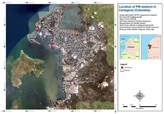
Figure 1.
Spatial distribution of PM2.5 and PM10 stations in Cartagena, Colombia.
The study is conducted in a sequential way considering several steps. In the first step, an assessment of the collection of PM pollutant data is carried out (PM2.5 and PM10) to statistically identify non-significant data. The next step consists of the imputation and completion of PM2.5 record series data. The last step consists of the determination of the main factors that cause asthma incidence, an estimation of the correlation between asthma incidence and PM2.5, as well as an estimation of health impact.
2. Methodology
The study area was the city of Cartagena, located in the Colombian Caribbean, (10°25′20″ N and 75°32′25″ W). Cartagena is a United Nations Educational, Scientific and Cultural Organization site (UNESCO). Cartagena is characterized by a tropical and warm climate, with an average annual temperature of 28 °C.
To deduce the variables of greater or lesser importance in childhood asthma exacerbation in the city of Cartagena, different statistical analyses were carried out on the data of PM2.5 concentrations and on the monthly incidence data for asthma.
In the first instance, an evaluation of the quality of the data was carried out to detect possible irregularities in the pollutant records and in the monthly incidence of childhood asthma (from 0 to 9 years old) cases reported in visits to hospital centres. A process of outlier elimination was performed, as was an evaluation of the quality of the air quality network by a density analysis. Subsequently, an attempt was made to increase the series of pollutant records by statistically imputing the missing data and the eliminated outliers. Once sufficiently long series of pollutants were obtained with data features parallel to the incidence, it was possible to determine the influence of PM2.5 on childhood asthma in Cartagena using bivariate analysis, spectral analysis, and visual and statistical correlations (Figure 2).
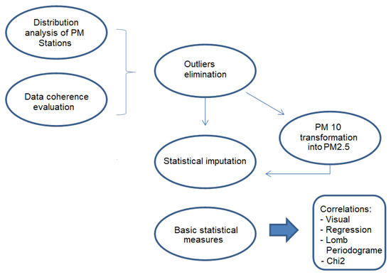
Figure 2.
Workflow in data analysis.
2.1. Data Source

Table 1.
Data source.
The spatial distribution of PM2.5 stations in Cartagena and the description of the location and type of measurement are reported in Figure 2 and Table 2.

Table 2.
Stations selected for data analysis. Source: EPA-Cartagena.
2.2. Feasibility of Recording Stations
The distribution of the PM stations was evaluated by kernel density analysis with the support of a Geographic Information System (ArcGis® 10.2.2). The kernel density tool was used [30]. A cartographic representation was made showing the PM stations together with the result derived from the kernel analysis. In this result, the values were displayed in 6 classes defined by the Natural Breaks function, which divides the classifications according to the distribution of values in a projected histogram. The minimum density value, tending to zero, was eliminated to clarify the cartography, showing it in a transparent way. This tool carries out a point density analysis (which would correspond to the PM stations, in this case) according to the kernel equation (Equations (1)–(4)) [31] calculating the magnitude of a variable times a unit area according to a Gaussian function variable in time (or in space), as follows:
where t is the time variable with value 0 for the case of study, x and y are the spatial coordinates and d is the Euclidean space. This can be used to solve a heat equation such as:
For t > 0 y x, y {\displaystyle x,y} x, y ∈, R d {\displaystyle \mathbb {R} ^{d}} , R d {\displaystyle\mathbb {R} ^{d}} where Δ {\displaystyle\Delta } is the Laplacian operator, with the initial condition:
where δ {\displaystyle\delta} is a Dirac delta distribution and the limit is taken as distribution. This becomes:
where φ is a soft compact support function.
At the time of conducting this study, the location of the measurement stations was conditioned to the knowledge and experience of the environmental authorities of Cartagena. Therefore, through this feasibility assessment, an attempt was made to find out if the selection of the location of the stations was adequate, and then proceed to offer solutions that would suggest a new distribution if necessary.
2.3. Evaluation of the Recorded PM2.5 Data
Another quality analysis of the PM2.5 data was mass balance using the double-mass technique [32], also known as double-mass analysis. This method is used to evaluate the internal coherence of the records by graphing and generating a coefficient of determination R2 by linear regression.
The results face accumulated frequency dispersion graphs of the PM2.5 records of two stations that must necessarily have similar geographic characteristics (altitude, orographic environment, differences in social environment) and that are not separated by more than 50 km. This method deduces that the variations in maximum and minimum, in the records, occur correspondingly, since they would be influenced by the same variations in atmospheric and social characteristics. The better the fit of the data in the theoretical regression line, the better the internal coherence of the data, while the existence of disparity and sudden breaks in the slope line between the records indicates probable errors in data collection.
The mass balance method has proven its usefulness for the records of climatic data measured in meteorological stations on a daily or monthly basis [33] and may be valid for fine particle records also due to the similarity of the recording process. This technique is a widely used method for the evaluation of the data records, which demonstrates a proper coherence and a good internal fit of the measurements [34,35].
2.4. Elimination of Outliers
The process of statistically purifying non-significant data was applied to the series of incidence data and the PM records in Cartagena. The process was developed from the statistical programming software RStudio [36]. Data above or below that 50% and outside a range of 1.5 times of the “whisker” were eliminated from the records of incidence for asthma and PM pollutants.
2.5. Imputation of Missing Records
The PM data series present a monthly scale and correspond to a period of 4 years (2014 to 2017), with some series with incomplete months, especially for 2017. Given that complete pollutant data series are required for the statistical analysis of this study, as well as for other types of analysis (such as air quality modelling), the missing data were completed by using equations of statistical imputation to obtain continuous series. In turn, the data eliminated after filtering statistically insignificant data were also imputed under this methodology. The imputation equations generate synthetic values compared to the mean values of the entire data series in correlation with a reference station whose record values must be complete, but above all, the process offers variability in the completed series. In order to evaluate the imputation analysis, some standard deviation parameters were calculated as an estimation of the error.
The imputation equation used is the one proposed by two specialists of the US Hydrological Service [10,12], is widely used in meteorology and hydrology, and is valid for recording pollutant particles [11] (Equations (5)–(7)).
where the coefficients and are calculated as follows:
where is the mean of the incomplete data series station, is the covariance of both stations, is the variance of both stations, and is the mean of the complete data series station.
These imputation equations were developed with Rstudio software, always in relation to a complete reference station. It should be noted that, in the series where there was no reference station to complete the data, it was necessary to use the arithmetic mean relative only to the month that needed to be completed. In the months of October, November, and December 2016 for the Bocana (GTC1) and Cardique (GTC3) stations, the monthly averages were also used to give some variability to the new data. In addition, the standard deviation of PM2.5 concentration observations at the measuring stations was estimated.
A series of criteria related to the reality of the Cartagena stations were followed to select which records with complete data could be used in the imputation of data from the incomplete stations. Several criteria were adopted. For the root mean square error of the mass balance between the stations (R2 > 0.7), the stations should not have an extreme topographic difference, there should not be different atmospheric characteristics, and finally they should not be located at places with different vehicle traffic volumes and different densities of industries.
Since the Policía Turística Station (GTCI5) only recorded PM10 data, the transformation ratio of the PM10 values into PM2.5 was used, and we defined the PM2.5 value as 50% of the PM10 value according to similar studies found in the literature [37,38].
Once the quality of the data recording process was evaluated through the distribution of stations and the internal coherence of the pollutant data series, these records were correlated and analysed bivariably with the monthly incidences of asthma obtained. The data used in the correlations were the complete series of incidence of asthma in children between 0 and 9 years (2014–2016) and the concentration of the pollutant PM2.5 (2014–2016). Despite the existence of pollutant records for 2017, it was decided not to include them in the correlation analysis in order to be able to compare them in a similar way with the incidence, due to data shortages in 2017. The 2017 time series are included in the rest of analysis.
2.6. Chi2 Analysis
To perform the Pearson Chi-square analysis (ꭓ2), the variables that had a greater influence on the development of asthma were determined, taking into account a cohort of 262 children from Cartagena, to verify the weight of traffic emissions in the diagnosis and evolution of the disease. Traffic emissions should be considered an important source of PM2.5 in Cartagena [39]. The statistical association between the dependent variable and the positive diagnosis of asthma due to the presentation of symptoms in the child, with each one of the independent or predictive variables of the disease, were analysed. In total, more than 200 variables that could be related to childhood asthma were analysed. Data collection for these variables was carried out from social surveys programmed in hospital centres for patients with asthma to study the living conditions and genetics of paediatric patients.
The function used for Pearson’s Chi-square (ꭓ2) bivariate analysis is shown in Equation (8).
where n is the observed frequency and corresponds to the theoretical frequency, while ꭓ2 is the theoretical statistic that is applied to decide whether or not a series of data fits a previously determined theoretical function.
2.7. Correlation
The correlation analysis had three independent processes that are exposed below.
First, a linear regression correlation was carried out to analyse the R2 coefficient, comparing the monthly incidence data and the mean values of PM2.5, also on a monthly scale. This correlation would demonstrate the degree of dependence of the incidence variable compared to the PM2.5 independent variable.
Second, a visual correlation was performed by comparing the graphs of mean PM2.5 concentration with the incidence of asthma in children between 0 and 9 years old in Adobe Illustrator software. The comparison periods were between 2014 and 2016. The analysis was carried out by comparing maximums and minimums in both graphs and joining them only if they corresponded temporarily.
As a third correlation process, the spectral analysis method was used. This analysis would demonstrate the correlation between the incidence of asthma and the PM2.5 concentration, aiming to recognize possible periodic elements in the variability of the study data.
Even though the periods considered for the analysis were quite small (3 full years), it should be noted that they are the best data available, as is usually the case in developing countries. The results derived from the spectral analysis yielded maximums and minimums with a determined periodicity that indicated the cycles not discernible to the naked eye and that corresponded to the usual extreme values.
The two variables (concentration and incidence) were analysed separately, without the need for linear or polynomial adjustments in any of them. If there were common periods in both analyses, the correlation could be demonstrated.
For this purpose, PAST software was used [40], which works with the Lomb–Scargle periodogram algorithm function that allows the obtainment of spectral diagrams with respect to time series with non-equidistant values [41,42]. A minimum significance is given (p value of <0.2) which accounts for lower periodicities, as these values are invalid.
The formula on which this periodogram is based can be observed in Equations (9) and (10). The PAST program returns periods with different powers, breaking up the superimposed cycles in the data series. The power in the results reflects the significance of the peak of each cycle. If the same spectral periods were found in different data series, a possible correlation between the two variables could be considered.
where is:
where mz and s2 are the estimated mean and variance of the data {z(t1), z(t2),…,z(tN)}.
wj is the angular frequency (cycles per radian), while ƒj = wj/(2) is the frequency in cycles per sampling interval. The parameter t makes the estimator I(wj) (Equation (9)) independent to time. I(wj) is the Lomb–Scargle periodogram for the frequency wj.
Subsequently, different basic statistics were calculated throughout the data series, including those that were completed using the imputation equations. Under the analysis with the Rstudio software, arithmetic means, medians, identification of maximums and minimums, means of the five maximum values, and means of the five minimum values were performed.
2.8. Interpolation
Various spatial interpolations of specific PM values of the five stations in Cartagena were carried out to observe how the spatial distribution of PM2.5 (μg/m3) concentration varies throughout the city. The interpolations were performed using the ArcGIS software with the inverse distance weighted method (IDW) tool, where the inverse of the distance is weighted linearly from pixel values for the whole sample [43]. The IDW method was chosen because it is an interpolation tool for location-dependent variables and because it is a preferable method for a network with a low number of information points, as with the case study at hand [44,45,46].
The interpolations included 5 scenarios: (1) interpolation of the arithmetic means for the period 2014–2016; (2) interpolation of the arithmetic means of the five maximum values for the period 2014 to 2016; (3) interpolation of the arithmetic means of the five minimum values for the period 2014 to 2016; (4) interpolation of the arithmetic means of the months corresponding to the favourable season for a higher concentration of PM2.5 (the dry season, from December to April); (5) interpolation of the arithmetic means of the months corresponding to the most propitious time for PM2.5 stagnation (the humid season, from August to November) [47].
The dry season and wet season scenarios were defined from the synoptic situation charts for Cartagena [47], defining the first as the period between the months of December and April and the second as the months of August to November.
2.9. BenMap Analysis
Finally, the health impact function was applied to estimate the number of avoidable cases of prevalence in childhood asthma considering reductions in PM2.5 concentrations to the WHO recommended limit (5 μg/m3 annual mean). In this regard, the Environmental Benefits Mapping and Analysis Program Community Edition (BenMap-CE) software was used. This is used to estimate the health impact resulting from changes in air pollution concentrations [48]. The concept of health impact function (HIF) was applied, the expression of which is deduced from the log-linear model C-R functions [48,49,50]:
where ∆y is the variation in the number of cases of the endpoint under study, ∆x is the variation in the concentration of the pollutant considered (PM2.5 in this case, in μg/m3), β is the epidemiological coefficient (adimensional) that is deduced from the corresponding epidemiological study, y0 corresponds to the base incidence of the disease considered, and Pop is the size of the population exposed to the pollutant (children aged from 0 to 9 years old).
3. Results and Discussion
3.1. Feasibility of Recording Stations
The kernel density analysis for the pollutant measurement stations shows results with different shades of colours meaning a gradual scale from higher density (red colour) to lower density (green colour), with values depending on the number of stations per area in the map. The highest density value occurs at the east of Bocagrande, on the Caribbean Sea, where there is no population, since there are two stations very close to each other in this area (Naval Base—GTC2, and Cardique—GTC3) (Figure 3). However, the second and third density values are in the urban area of the city. These values coincide with the highest concentration of population and, in turn, coincide with most of the neighbourhoods in Cartagena.
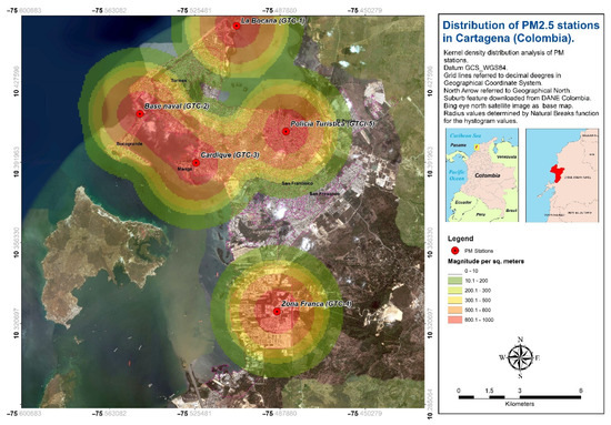
Figure 3.
Density analysis and location of PM measurement stations in Cartagena.
Some areas, such as the neighbourhoods of Sucre and Arroz Barato in the southeast of the city, or El Pozón and José Obrero, to the Northwest, were left with a very low or null density of stations, so they can be considered as areas with a low coverage of measurement.
Therefore, the maximum values coincide with most of the Cartagena population density (except for the highest density value, which occurs in the Caribbean Sea). The PM2.5 station network in the city is adequately distributed and its coverage is acceptable to carry out a data analysis or a possible modelling of air quality. However, there are certain areas with a lack of station coverage, i.e., in the southeast, northeast and northwest of the city, in the urban edge areas. To improve the network stations, it is recommended to locate a station to the northeast of the city (between the neighbourhoods of El Pozón and José Obrero) and another to the north of Mamonal or southeast of Cartagena (between the neighbourhoods of Sucre and Arroz Barato), as places with considerable population density.
3.2. Evaluation of the Recorded PM2.5 data
Mass balances analyses were carried out to demonstrate the internal coherence of the pollutant registration series (Figure 4). All the analyses had a determination coefficient R2 greater than 0.9. It is observed that some graphs present slight changes in slope that could indicate an alteration in the records, but most of them do not show any “break” in the slope. This occurs in the middle section of the mass balances between the Zona Franca and the Naval Base, between the Naval Base and Cardique, and between Cardique and Zona Franca, but it is not observed between the Bocana and the Naval Base.
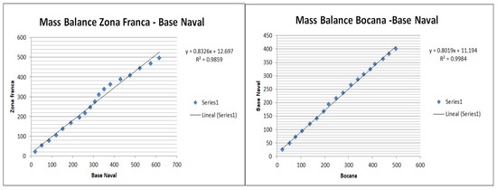
Figure 4.
Mass balances for different combinations of PM2.5 (µg/m3) stations.
The mass balance between stations revealed excellent internal consistency in the data log measurements. Using this method, it is not possible to ensure that the stations are measured correctly. However, it can be affirmed that the registered values are homogeneous and consistent with each other. It is possible to say that the coherence of the data recording between stations is practically optimal. Further research is needed to evaluate the possibility that all stations have the same measurement error. Therefore, the most plausible hypothesis is that the stations register the data correlatively with a similar variability. Changes in slopes could identify an error in the internal coherence of the data, but the fact that they occur in the three stations simultaneously and during a relatively short period of time can lead to the assumption that they are due to a change in the trends of PM pollutants due to abnormal atmospheric situations [32].
3.3. Elimination of Outliers
The clearance analysis for paediatric monthly incidence did not reveal any statistically non-significant or out-of-range data (Figure 5). Therefore, no values were eliminated from the data series. The analysis of outliers of the concentration records (Figure 5) revealed a total of nine non-significant data. These were values such as 42.5 μg/m3 of PM2.5 concentration for the Cardique station, 52.7 and 48 μg/m3 of PM2.5 concentration for the Base Naval station, and the value of 30 μg/m3 for the Policía Turística station. The Zona Franca station and the mean of all stations did not reveal out-of-range values (Table 3). These non-significant values were eliminated from the statistical analysis carried out later.

Figure 5.
Outliers revealed in debug function for PM2.5 pollutant records (A) and monthly incidence (B).

Table 3.
Non-significant values (μg/m3) statistically found in pollutant records, accompanied by standard deviation (Std.).
3.4. Imputation of Missing Data
The data imputation was carried out considering the five stations and obtaining a complete series of data from 2014 to 2017. Assuming 48 months of records and a total of 288 data altogether, the number of imputed data was 86 (29.86% of the total (Table 4)). This could be considered quite a high percentage; nevertheless, most of the imputed data are from some months at the end of the 2017, and were not used in the correlation study. Therefore, excluding the missing data from 2017, 50 values would have been completed out of a total of 216 (23.15%). The statistical imputation gives a series of data that are highly smoothed, without having sufficient variability of maximums and minimums. In other cases, the monthly variability is collected considerably well, as is the case of the imputation for the Naval Base station.

Table 4.
Result of the concentration data record with the statistical imputation of missing data. Statistically non-significant data in red; data completed with statistical imputation in green; data completed through monthly averages in pink.
It is quite accurate to point out that the stations present a good quality in the data record. This fact, added to the acceptable spatial distribution of the monitoring network in the city of Cartagena, validated and justified the imputation process of the data in the correlation analysis carried out. Some eliminated data helped to improve the basic statistics and the quality of the series since they were considered statistically insignificant and could create “noise” in the total set. Although minimal data were removed and overall trends were appreciably unchanged, this is a basic statistical process that should be applied as part of a common workflow [1].
Statistical imputation was performed according to basic data completion equations. Subsequently, it was possible to overcome the statism characteristics of single-year values. Despite the high number of imputed data and the loss of reliability in this regard, the results showed good variability, without being an excessively smoothed completed series. Accordingly, they could properly fit to the seasonal reality of Cartagena.
3.5. Chi2 Analysis
Among the 58 environmental variables analysed, without considering the genetic family variables, the variable “Flow of vehicles per day” occupies the ninth position in importance in the association degree with asthma, presenting an 85% association with symptoms among the children studied (Figure 6 and Table 5) using SPSS v24.0 [51].
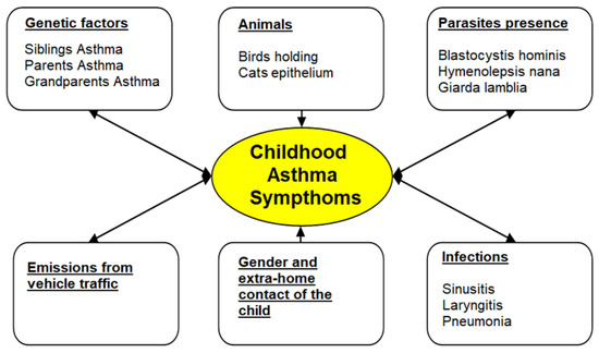
Figure 6.
Statistically significant variables (p < 0.20) in a cohort of children up to 4 years in Cartagena, Colombia.

Table 5.
Results of Pearson’s Chi2 analysis.
The Chi2 techniques applied were adequate for determining the main variables on which childhood asthma in Cartagena is dependent. Genetic factors, the possession of domestic animals and the presence of parasites were the main causes of asthma in Cartagena. However, these variables are difficult to quantify, as they depend on social factors and genetic inheritance.
3.6. Correlations
Linear regression analysis between monthly asthma incidence and PM2.5 concentration records resulted in a low R2 (0.0048). There is a great dispersion in the data analysed, although a slightly positive slope is observed, which leads us to think that increasing the concentration of the pollutant PM2.5 would slightly increase the incidence of paediatric asthma (Figure 7).
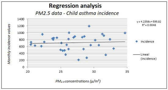
Figure 7.
Results of linear regression of PM2.5 pollutant and monthly incidence of paediatric asthma.
The visual correlation allows us to discover the maximum coincidental points and temporary analogies between the incidence of childhood asthma and the concentration of particles (Figure 8 and Table 6). In total, 13 significant maximums and minimums were observed in the asthma incidence data and 18 maximums and minimums were observed in the pollutant records between 2014 and 2016. The visual analysis showed six corresponding maximums and five minimums in both graphs, nine of them very poignant. Notably, 61% of the maximums and minimums occurred coincidentally in both data series. Most of the positive correlations were found between January 2014 and March 2015 (seven of them), while the rest occurred between December 2015 and August 2016 (the four remaining). Most of the coincidences of the maximum in the concentration of pollutants with the maximum in the incidence of asthma (up to five of them) occurred from December 2014 to April 2015. It is possible to determine a certain lag in time between the pollutant records and the incidence. Apparently, the increase or decrease in the concentration of PM2.5 would occur first, and later the incidence would increase or decrease.
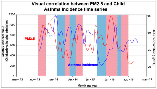
Figure 8.
Visual correlation of the series of PM2.5 (µg/m3) concentration and incidence of asthma. Blue lines represent childhood asthma incidence hospital admissions, red line represents average PM2.5 values, red (blue) rectangles show matching periods of high (low) PM2.5 values and high (low) incidence, and red and blue arrows represent a matching period but with a lag.

Table 6.
Maximum and minimum periods found for asthma incidence and PM2.5 values. Max.—Maximum; Min.—Minimum; Incid.—Incidence; PM.—Particulate Matter.
In the spectral analysis of PM2.5 concentrations (Figure 9), four maximum values are found that reach or exceed the significance line (p value < 0.2 or 6.5). The periods found in this analysis correspond to 0.91, 0.87, 0.12 and 0.09 years. Therefore, it is possible to ensure that every 0.91 and 0.09 years certain maximums in concentration occur with sufficient statistical significance, while the values of 0.87 and 0.12 should not exceed the minimum significance. The spectral analysis (Figure 9) of the monthly incidences of asthma reveals three maximum values. The periods shown are: 1, 0.97, and 0.02 years. Therefore, it is possible to affirm that, every 0.97 and 0.02 years, maximum values occur in the incidence of asthma.
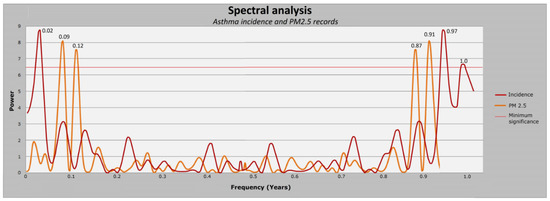
Figure 9.
Spectral analysis for PM2.5 monthly maximum records and for child asthma monthly incidence. Red line indicates minimum statistical significance.
3.7. Basic Statistics
Statistics revealed general mean values between 21.70 and 33.16 μg/m3 of PM2.5. The means of the five maximum values revealed ranges between 25.9 and 48.6 μg/m3, while the mean of the five minimum values showed less variability between stations with a range of between 16.56 and 18.04 μg/m3 of PM2.5 concentration. The difference between the mean of the dry and humid seasons was not significant (less than three points of PM2.5 value) in most of the stations with the exception of Zona Franca and Cardique (between five and sevent points of difference) (Table 7).

Table 7.
Basic statistics of PM2.5 pollutant records (μg/m3) in the city of Cartagena.
Basic statistics consider the mean, median, maximum and minimum values of the incidence of childhood asthma (Table 8) considering both the dry and wet seasons.

Table 8.
Basic asthma incidence statistics in Cartagena.
3.8. Interpolation
Up to five results were obtained from various PM2.5 scenarios. The arithmetic means of the interpolations varied in a range between 21 and 34 μg/m3 of PM2.5. It is possible to see that the station with the lowest PM2.5 mean value was Olaya—Policía Turística, while the one with the highest values was Mamonal—Zona Franca.
The interpolation for the maximum values reflects ranges between 25 and 50 μg/m3 of PM2.5, which is a very remarkable range of variation. The highest values again occur at the Mamonal—Zona Franca station, with the lowest occur at the Olaya—Policía Turística station. There is a range of values that exceed 35 μg/m3 from the north of the city to the east, passing through the historical city centre. It is the strip that covers the largest populated area of the city.
The minimum PM2.5 values are more stable and relatively close to each other, being in a range between 16 and 19 μg/m3 of PM2.5. In this case, it is the Cardique station that presents the lowest values, while the highest values are presented by La Bocana and Olaya (Policía Turística) together with the Mamonal—Zona Franca station. During the wet season, the values vary between 20 and 28 μg/m3 of PM2.5. Again, the highest concentrations are in Mamonal—Zona Franca, next to La Bocana station. In the dry season, the values have a greater disparity, between 20 and 35 μg/m3 of PM2.5. It is the Olaya—Policía Turística station that presents the lowest values and that lowers the range, since the rest of the stations exceed 25 μg/m3 of PM2.5. Again, it is Mamonal—Zona Franca that registers values up to 34 μg/m3 (Figure 10 and Figure 11).
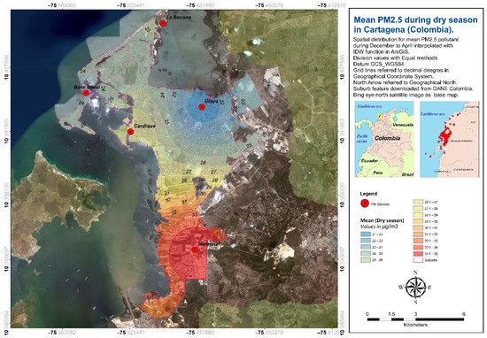
Figure 10.
Mean PM2.5 values during dry season in Cartagena (Colombia).
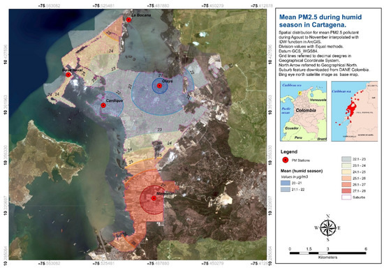
Figure 11.
Mean PM2.5 values during wet season in Cartagena (Colombia).
3.9. Health Impact on Childhood Asthma
Considering the guidelines contemplated by the World Health Organization (WHO), the reduction in anthropogenic PM2.5 concentrations to safe levels (5 µg/m3) would avoid approximately 240 (95% CI: 137–330) annual cases of childhood asthma, taking into account emergency room visits, which would represent an important advance in health in the city (Figure 12).
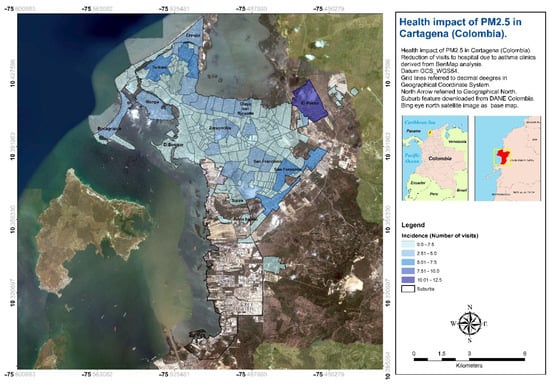
Figure 12.
Number of childhood asthma cases avoided if PM2.5 levels had met the standards recommended by WHO.
Child population exposure to PM2.5 was specified at neighbourhood level by interpolating annual average records using Voronoi interpolation (Voronoi neighbourhood averaging, VNA). VNA is an algorithm used by BenMAP-CE to interpolate air pollution monitoring data to an unknown location [48]. In this way, the spatial distribution of PM2.5 can be known across neighbourhoods (Figure 13).
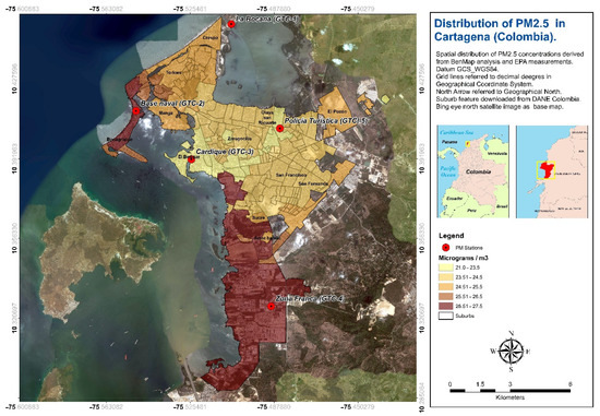
Figure 13.
Airborne distribution of PM2.5 in Cartagena through Voronoi interpolation (Colombia).
The value of the epidemiological coefficient (β) corresponding to asthma visits was deduced from previous epidemiological studies, as is usual in this type of project. In this case, the value of the epidemiological parameter (β) is 0.0147117 (σ = 0.0034923: error follows a normal distribution) [52].
Once the model was applied, it was observed that the neighbourhoods most affected in terms of impact on health were those with the lowest socioeconomic status (El Pozón, Torices, San Fernando). The main limitation of the use of the log-linear model in this case is the constant value of the incidence in the entire city, corresponding to one hospital visit for every 166 children. However, the population was considered from 0 to 9 years old, varied by neighbourhood.
Despite the fact that Zona Franca has the highest levels of PM2.5, the model showed a null value due to the absence of population in this industrial area.
4. Discussion
Considering the bivariate analysis study, it can be concluded that the hereditary genetic component is a relevant variable when trying to explain the development of asthma in Cartagena, taking into account that the association is statistically significant when analysing the relationship between the child under study and brothers and grandparents. This result is assumed at the international level because it is well known that the genetic factor significantly influences the onset of the disease [53,54,55,56].
However, although it is the most important cause, the genetic factor is not the only influence on the appearance of asthma in Cartagena. Other variables are also presented that would explain the symptoms indicative of the disease in childhood, although with a relative weight not equally important. In any case, the analysis here reveals that PM2.5 generated by road traffic would influence the appearance of symptoms of childhood asthma, a situation that is frequently reproduced [57,58,59,60].
The linear regression correlation between the PM2.5 contamination records and the incidence of asthma obtained a low R2 coefficient (0.0048 or 0.48%), probably because PM2.5 contamination is not the only cause in the incidence of paediatric asthma, which is usually explained by a conjunction of more than 200 variables. Linear regression in fine particulate health impact studies usually reveals very low R2 values [61,62].
The visual correlation showed a considerable influence of PM2.5 on the incidence of childhood asthma due to the great correspondence between the maximum and minimum of both variables. Subsequent correlations indicated that the influence in exacerbation of asthma may be seasonal. Spectral analysis gave certain common periods in asthma incidence and pollutant records.
In turn, it is possible to affirm the existence of three maximums and two minimums that would present a correlation with a certain time lag. This lag occurs in the order of a maximum of one month. The increase or decrease in PM2.5 concentrations is prior to the variation in the incidence of asthma in all cases, except in the case of the minimum of PM2.5 in January 2016, which was preceded by a decrease in incidence in December 2015. This last coincident minimum may be due to a minimum incidence of PM2.5 as a result of unrelated causes, since PM2.5 does not seem to be related to the incidence in this case.
In the case of the rest of the minimums and maximums found to coincide with a time lag, it can be observed how PM2.5 concentrations precede the increase or decrease in the incidence. This fact could be explained by the airway inflammation process caused by the air pollutant during a long time of exposure [63]. The time from the moment the child breathes PM2.5 until airway inflammation and hospital visit occurrence could take several days, since normally the patient does not go to the emergency room immediately after inhalation of the pollutant, but when the symptomatology and the clinical process evolve [64].
In many cases, the alveolus will not corrode by the action of PM2.5 if the atmospheric situation and, therefore, the accumulation of polluting particles, is not maintained for several weeks. Some studies in China [65] and the U.S. [66] have observed that the time lag between the increase in PM2.5 and the hospital visit can be up to 14 days. Therefore, the lag could come from the time elapsed until the appearance of symptoms or the exposure time necessary for the affection to occur at the lung level.
Another possibility that would explain the lag between these minimums and maximums would come from the time scale of the analyses. Both the asthma incidence data source and PM2.5 data have been offered to the public in a format with a monthly scale; therefore, it is not possible to assign a specific time lag, as could be performed if the data had a daily scale. While certain studies did not find a lag between the incidence of asthma and PM2.5, such as the one carried out in Taiwan [67], other studies for Reno [68] and Phoenix [69], U.S.A., previously assumed a lag of 2 to 3 days between the increase in air pollutants and the incidence of asthma.
It is possible to confirm that with a greater temporal resolution of asthma incidence and PM2.5 data, the existence of the time lag could be observed, and we could assign a specific time period for it. For this, it would be necessary to carry out new collections of hospital data and PM2.5 measurements.
There were two maximum values that could be considered contemporary and common between the variables of pollutants and asthma incidence. These periods given by the program can be translated into an occurrence of a maximum every year (0.95 years) and another every 25 days (0.07 years).
The fact that there are maximum values in two similar periods of the two variables analysed is an indication of a probable influence of PM2.5 on the incidence of childhood asthma. Consequently, the correlation between both variables would be demonstrated at least seasonally. Each year, there would be a maximum in the influence of pollutants on childhood asthma which could correspond to any of the summer situations of the so-called “dry season”, between the months of December and April [47], in which normal atmospheric situations correspond to a stable atmosphere, without low pressures that favour precipitation and, therefore, the removal of particles in suspension in the atmosphere, or convective situations that create mixing in the atmospheric air layers.
The above statement can be determined by analysing the correspondence between the results of the spectral analysis, but it can also be confirmed through the visual correlation analysis. In this correlation, it is highlighted that most of the coincidences of the maximum in the concentration of pollutants with the maximum in the incidence of asthma (up to five of them) occur during the months of the dry season (December to April). Meanwhile, most of the minimums coinciding between the incidence and the concentration of pollutants occur in a scattered way between the wet season (April–June), and the so-called transition times. Two of the coincident maximums also occur outside the periodic range of the dry season, perhaps correlated with other atmospheric or social situations that have not been determined. Meteorological variables in Cartagena de Indias have already been established as leading factors for increasing and decreasing PM2.5 values [70]; therefore, dry and wet seasons must have a noticeable influence in air quality levels and childhood asthma incidence. In other world regions, relationships between PM2.5 and meteorological dynamics have also been found in Hong Kong [71] in a positive correlation for pressure and a negative correlation for temperature. For 68 major cities in China, it was found a negative correlation between temperatures and PM2.5 in autumn but the opposite during winter, as relative humidity was positively related to this pollutant [72].
The secondary maximums that coincided every 25 days could not be attributed to a summer synoptic situation. However, it could be thought that since the period was close to representing the range of days of a month in the calendar (30 days), it could be more associated with a social situation where road traffic or industrial activity increases.
In any case, the data analysed with the correlation techniques and Chi2 lead us to think that PM2.5 has an important influence on childhood asthma.
The level of the correlations and the bivariate analysis carried out are reported in Table 9 by weighting the analysis and the obtained results.

Table 9.
Weighting of the probability of the demonstration of the influence of PM on the monthly incidence of asthma in children between 0 and 9 years old.
The bivariate analysis was divided into 58 main variables, assigning a percentage value in descending order to each of them based on position, with the first variable with the highest coincidence (asthma for siblings) having a value of 100% and decreasing according to the importance in an order of 1.8% (result of the weighted division of 100% between 58 variables). Consequently, the variable “Vehicle flow per day” obtained a coincidence assessment of 85.5%.
In the analysis of the basic statistical values, it can be seen how during the dry seasons the average monthly incidence of asthma tends to rise, while in the wet season it tends to decrease. These facts are coincident with the mean values of PM2.5, which rise in the dry seasons while they decrease in the wet ones. Nevertheless, some stations present a very low range of change between the means during both seasons. This could be because the maximums and minimums in the values may be hidden by specific atmospheric or social situations since the average is carried out considering all the data.
The visual correlation showed 11 coincident maximums and minimums out of a total of 13 for the incidence and another 18 for the PM2.5 records, which was quantified with a percentage (minimum) coincidence of 61.1%. While the correlation by spectral analysis showed agreement in three of four maximums with sufficient significance (75% of agreement). Spectral analysis has proven to be an effective tool for deducing the influence of different factors into climate [17,73] and air quality [15].
The total mean of the coincidence that can be taken as the probability of influence of PM2.5 in the monthly incidence of asthma turned out to be 55.50%, so it can be stated that PM2.5 exerts a significant influence on asthmatic incidence at least for the first age group of children in Cartagena. Statistical assessments of the relationships between childhood asthma and PM exposure within one or two weeks have been carried out in the Chinese regions of Taiwan [74] and Xiamen [65]. Both analyses were in agreement with the present study by showing a relationship between episodes of high PM2.5 and PM10 values and an exacerbation of childhood asthma. This was also the case for other regions in the world such as Seoul in South Korea [7], and Seattle in the U.S.A. [52], where an increase of 11 µg/m3 in PM had an associated OR of 1.15 (95% CI: 1.08 to 1.23).
Mathematical correlations and influence analysis not only supply simple visual or graphical correspondence, but also support scientific evidence of a physiological nature [63], for example, whereby PM2.5 particles penetrate deep into the lung, irritating and corroding the alveolar wall, and other types of analytical evidence [69]. The correlations of this study could reinforce theories of physiological influence when empirically verified with statistical data.
PM2.5 sources in Cartagena de Indias have been established to have a mainly road traffic origin and to be distributed near the main roads. Higher values are concentrated in the northwestern and southeastern city areas [39]. This concentration distribution matches the estimations made in the present study through interpolation models in GIS, where northwestern and southern areas have higher PM2.5 values.
Comparisons in BenMap regional results are difficult due to the different social patterns that could be present. Davidson et al. [75] found that reducing PM2.5 to 12 µg/m3 would lead to a reduction of 2000 premature deaths in the state of California (U.S.A.), meaning nearly 10 times the reduction in Cartagena, but for a population 39 times greater.
Some shortcomings were taken into consideration when analysing the data. First of all, imputed data from missing and eliminated values represent an estimation and, therefore, caution in the statistical analysis was applied. To solve this issue, only average values of all the PM stations were used in correlations, instead of using single values.
Estimations were also used for the transformation of PM10 into PM2.5 values. These estimations are supported by published works in similar regions for the mathematical analysis of Cartagena city. Discarding the PM10 time series would have made it impossible to conduct this research due to the scarce data.
Mass balances are a widely used and outstanding technique for meteorological data assessment. However, some issues could be found when the accumulated values are very low or near 0, because too many “breaks” are visualized. The opposite occurs when high values are included in data series. Fortunately, intermediate values were recorded in the PM measurement stations.
5. Conclusions
The aim of this study was to provide a comprehensive spatial–temporal data analysis of PM2.5 and the incidence of childhood asthma through different correlations in a developing country in which a lack of data prevents the proper inference and monitoring of public health. The interpolations and the basic statistics calculated for the PM2.5 values show three relevant results. This study has proven to be an effective workflow for the treatment and standardization of data prior to any possible use, for example, for air quality modelling studies.
The correlation analysis performed in this study showed a good agreement between childhood asthma incidence and PM2.5 values. Chi2 had the best fit between both variables with 85.5% of coincidence, followed by spectral analysis with 75% similarity. Visual correlation, averages and linear regression analysis showed lower coincidences with 61.1%, 55.5% and 0.48%, respectively, but this may have been due to multiple variables (not only PM2.5) that could have caused greater influence together. As childhood asthma could be related to PM2.5, a BenMAP analysis was carried out to estimate the health benefits of the reduction in that pollutant in Cartagena de Indias. If PM2.5 is reduced to safe values (5 µg/m3), nearly 240 annual cases of childhood asthma could be prevented.
Performing these statistical analyses served, to a great extent, to increase the amount of data available, filter out invalid data, and justify the dependence of childhood asthma variables on vehicle emissions in Cartagena. The analysis and pre-processing of air quality data series is a very important phase in developing countries, as the lack of technical resources results in considerable data loss. Therefore, this study could be considered a benchmark for studies focused on the health impact of air pollutants at urban scales in developing countries.
Author Contributions
Conceptualization, J.A.Á.A., A.F.S. and M.S.; methodology, J.A.Á.A. and A.F.S.; software, J.A.Á.A. and A.F.S.; validation, M.S., E.Q.B. and L.R.C.; formal analysis, J.A.Á.A., A.F.S. and M.S.; investigation, J.A.Á.A., A.F.S. and M.S.; resources, M.S., J.A.Á.A., E.Q.B. and L.R.C.; data curation, J.A.Á.A. and A.F.S.; writing—original draft preparation, J.A.Á.A., A.F.S. and M.S.; writing—review and editing, All authors.; funding acquisition, M.S. All authors have read and agreed to the published version of the manuscript.
Funding
This research herein presented is granted by the ELARCH scholarship and mobility, a project funded under the Erasmus Mundus Action 2 Partnership (EMA 2) by the European Commission and coordinated by the University of Basilicata. ELARCH Project: Reference number 552129-EM-1-2014-1-IT-ERAMUNDUS-EMA21 funded with the support of the European Commission.
Institutional Review Board Statement
The study was conducted in accordance with the Declaration of Helsinki and was approved by The Ethics Committee of the “Fundación Santa Fe de Bogotá”, Bogotá-Colombia (CCEI-282-206).
Informed Consent Statement
All families received an explanation about the investigation and signed a written informed consent to participate.
Data Availability Statement
The dataset used and/or analysed during the current study is available from the corresponding author on reasonable request.
Acknowledgments
This research has been made possible thanks to the Immunological Research Institute dependent of the Cartagena University Medicine School. In addition, the authors also want to thank the Health and Social Protection Ministry of the Colombian Republic for the provided data in the realization of the present study.
Conflicts of Interest
The authors declare no conflict of interest.
References
- OCDE. Recomendación del Consejo de la OCDE Sobre Buenas Prácticas Estadísticas; 2015. [Google Scholar]
- Heads of the National Statistical Institutes. European Statistics For the National Statistical Authorities; Luxembourg, 2017. [Google Scholar] [CrossRef]
- Martini, F.M.S.; Hasenkopf, C.A.; Roberts, D.C. Statistical analysis of PM2.5 observations from diplomatic facilities in China. Atmos. Environ. 2015, 110, 174–185. [Google Scholar] [CrossRef]
- Iordache, Ş.; Dunea, D. Cross-spectrum analysis applied to air pollution time series from several urban areas of Romania. Environ. Eng. Manag. J. 2013, 12, 677–684. [Google Scholar] [CrossRef]
- Bathmanabhan, S.; Madanayak, S.N.S. Analysis and interpretation of particulate matter—PM10, PM2.5 and PM1 emissions from the heterogeneous traffic near an urban roadway. Atmos. Pollut. Res. 2010, 1, 184–194. [Google Scholar] [CrossRef]
- Broome, R.A.; Fann, N.; Navin, T.J.; Fulcher, C.; Duc, H.; Morgan, G.G. The health benefits of reducing air pollution in Sydney, Australia. Environ. Res. 2015, 143, 19–25. [Google Scholar] [CrossRef]
- Kim, H.; Kim, H.; Park, Y.; Lee, J. Assessment of temporal variation for the risk of particulate matters on asthma hospitalization. Environ. Res. 2017, 156, 542–550. [Google Scholar] [CrossRef]
- Ritchie, H.; Roser, M. Outdoor Air Pollution. Our World in Data 2019. Available online: https://ourworldindata.org/outdoor-air-pollution (accessed on 14 May 2022).
- World Health Organization for the Western Pacific. Improving Data Quality: A Guide for Developing Countries; World Health Organization for the Western Pacific: Manila, Philippines, 2003; Volume 6, p. 74. ISBN 9290610506. [Google Scholar]
- Enders, C.K. Applied Missing Data Analysis; The Guilford Press: New York, NY, USA, 2015. [Google Scholar] [CrossRef]
- Yunus, R.M.; Zubairi, Y.Z. A probability distribution-based approach to impute missing values in hourly PM10 concentration. Integr. Catchment Assess. Manag. (iCAM) 2019, 10, 6. [Google Scholar]
- Paulhus, J.L.H.; Köhler, M.A. Interpolation of missing precipitation records. Mon. Weather Rev. 1952, 80, 129–133. [Google Scholar] [CrossRef]
- Iancu, I.; Canureci, G.; Iancu, E.; Vinatoru, M.; Street, P.R.; Street, D. Spectral Analysis of the Heart Sounds for Medical Diagnosis. In Proceedings of the 4th WSEAS/IASME International Conference on DYNAMICAL SYSTEMS and CONTROL, Corfu, Greece, 26–28 October 2008; Volume 1, pp. 61–65. [Google Scholar]
- Wolff, H. Spectral analysis of clinical signals: An interface between medical statisticians and medical engineers. Stat. Methods Med. Res. 1996, 5, 51–66. [Google Scholar]
- Tchepel, O.; Borrego, C. Frequency analysis of air quality time series for traffic related pollutants. J. Environ. Monit. 2010, 12, 544–550. [Google Scholar] [CrossRef]
- Dutton, S.J.; Rajagopalan, B.; Vedal, S.; Hannigan, M.P. Temporal patterns in daily measurements of inorganic and organic speciated PM2.5 in Denver. Atmos. Environ. 2010, 44, 987–998. [Google Scholar] [CrossRef]
- Fernández-Sánchez, A.; Martín-Chivelet, J. Revisión de la estratigrafía del δ 18 O en sondeos de hielo de glaciares de los Andes Centrales: Implicaciones para la variabilidad climática del Holoceno. Geotemas 2016, 16, 565–568. [Google Scholar]
- Niklasson, U. Spectral Analysis of the Heart Rate Variability A Methodological Study av. Umea Univ. Med. Diss. 1993, 371, 59. [Google Scholar]
- Hou, F.H.; Ye, J.Q.; Chen, Z.G.; Cheng, Z.Y. Advances on enzymes and enzyme inhibitors research based on microfluidic devices. Yaoxue Xuebao 2010, 45, 694–698. [Google Scholar] [CrossRef]
- Lin, Y.; Chu, H.; Wu, C.; Chang, T. Hotspot Analysis of Spatial Environmental Pollutants Using Kernel Density Estimation and Geostatistical Techniques. Int. J. Environ. Res. Public Health 2011, 8, 75–88. [Google Scholar] [CrossRef] [PubMed]
- López-Aparicio, S.; Vogt, M.; Schneider, P.; Kahila-Tani, M.; Broberg, A. Public participation GIS for improving wood burning emissions from residential heating and urban environmental management. J. Environ. Manag. 2017, 191, 179–188. [Google Scholar] [CrossRef]
- Silverman, R.A.; Ito, K. Age-related association of fine particles and ozone with severe acute asthma in New York City. J. Allergy Clin. Immunol. 2010, 125, 367–373.e5. [Google Scholar] [CrossRef] [PubMed]
- Ding, L.; Zhu, D.; Peng, D.; Zhao, Y. Air pollution and asthma attacks in children: A case–crossover analysis in the city of Chongqing, China. Environ. Pollut. 2017, 220, 348–353. [Google Scholar] [CrossRef] [PubMed]
- Malig, B.J.; Green, S.; Basu, R.; Broadwin, R. Coarse particles and respiratory emergency department visits in California. Am. J. Epidemiol. 2013, 178, 58–69. [Google Scholar] [CrossRef] [PubMed]
- Tian, Y.; Xiang, X.; Juan, J.; Sun, K.; Song, J.; Cao, Y.; Hu, Y. Fine particulate air pollution and hospital visits for asthma in Beijing, China. Environ. Pollut. 2017, 230, 227–233. [Google Scholar] [CrossRef]
- Barnett, S.B.L.; Nurmagambetov, T.A. Costs of asthma in the United States: 2002-2007. J. Allergy Clin. Immunol. 2011, 127, 145–152. [Google Scholar] [CrossRef]
- Caraballo, L.; Zakzuk, J.; Lee, B.W.; Acevedo, N.; Soh, J.Y.; Sánchez-Borges, M.; Hossny, E.; García, E.; Rosario, N.; Ansotegui, I.; et al. Particularities of allergy in the Tropics. World Allergy Organ. J. 2016, 9, 20. [Google Scholar] [CrossRef] [PubMed]
- Luis, S.; Hoyos, M.; Navarro, J.O. Informe Consolidado Año 2016; EPA-Cartagena: Cartagena de Indias, Colombia, 2016.
- Hoyos, S.L.M.; Pájaro, N.C.; Navarro, J.O.; López, E.L. Calidad del Aire de Cartagena 2016; EPA-Cartagena: Cartagena de Indias, Colombia, 2016.
- ArcMap. How Kernel Density model works? ArcGis Desktop 2019. Available online: https://desktop.arcgis.com/es/arcmap/latest/tools/spatial-analyst-toolbox/how-kernel-density-works.htm (accessed on 14 May 2022).
- Vergne, M.; Berline, S.N.; Getzler, E. Heat Kernel and Dirac Operators; Springer: Berlin/Heidelberg, Germany, 1996; Volume 58, ISBN 978-3-540-53340-5. [Google Scholar]
- Searcy, J.K.; Hardison, C.H. Double-Mass Curves. WaterSupply Pap. 1960, 1541B, 31–66. Available online: http://udspace.udel.edu/handle/19716/1592 (accessed on 14 May 2022).
- World Meteorological Organization. Guide to Climatological Practices, Second Edition, 100th ed.; WMO: Geneva, Switzerland, 1983. [Google Scholar]
- Urrutia, J.A.; Palomino, R.; Salazar, H.D. Metodología para la imputación de datos faltantes en metereología. Sci. Tech. 2010, 17, 44–49. [Google Scholar]
- Gao, P.; Li, P.; Zhao, B.; Xu, R.; Zhao, G.; Sun, W.; Mu, X. Use of double mass curves in hydrologic benefit evaluations. Hydrol. Process. 2017, 31, 4639–4646. [Google Scholar] [CrossRef]
- RStudio Team. RStudio: Integrated Development for R; RStudio, Inc.: Boston, MA, USA, 2015; p. 10. Available online: http://www.rstudio.com/ (accessed on 14 May 2022).
- Medina, G.V. Determinación de la Correlación Entre PM2.5 y PM10 en el Distrito de San Isidro en Lima—Perú, 2016; Universidad Científica del Sur: Villa el Salvador, Peru, 2017. [Google Scholar]
- D’innocenzio, L.E.; Difilippo, F.; Lepore, P. PM10 and PM2.5 concentrations in Urban Air Size Fraction Distribution of Toxic Metals. Ann. Chim. 1998, 88, 281–289. [Google Scholar]
- Aldegunde, J.A.Á.; Álvarez, V.; Bolaños, E.Q.; Saba, M.; Atencio, C.H. Estimation of the Vehicle Emission Factor in Different Areas of Cartagena de Indias. Rev. Cienc. 2020, 23, 53–73. [Google Scholar] [CrossRef]
- Hammer, P.D.R.Ø.; David, A.T. Harper, Past: Paleontological Statistics Software Package For Education and Data Analysis. Paleaeontologia Electron. 2001, 4, 9. [Google Scholar]
- Polanco-Martínez, J.M. Estimación espectral de datos ambientales no equispaciados vía el periodograma suavizado de Lomb-Scargle. Una breve revisión. Analítika 2014, 8, 7–23. [Google Scholar]
- Lomb, N.R. Least-squares frequency analysis of unequally spaced data. Astrophys. Space Sci. 1976, 39, 447–462. [Google Scholar] [CrossRef]
- Esri. ArcMap 10.5. ESRI; ESRI: Redlands, CA, USA, 2017. [Google Scholar]
- de Mesnard, L. Pollution models and inverse distance weighting: Some critical remarks. Comput. Geosci. 2013, 52, 459–469. [Google Scholar] [CrossRef]
- Li, J.; Heap, A.D. A review of comparative studies of spatial interpolation methods in environmental sciences: Performance and impact factors. Ecol. Inform. 2011, 6, 228–241. [Google Scholar] [CrossRef]
- Li, L.; Zhou, X.; Kalo, M.; Piltner, R. Spatiotemporal Interpolation Methods for the Application of Estimating Population Exposure to Fine Particulate Matter in the Contiguous U.S. and a Real-Time Web Application. Int. J. Environ. Res. Public Health 2016, 13, 749. [Google Scholar] [CrossRef] [PubMed]
- CIOH. Climatología Y Situaciones Sinópticas en Cartagena de Indias, Colombia; CIOH: Cartagena de Indias, Colombia, 2008. [Google Scholar]
- EPA. Benefits Mapping and Analysis Program (BenMAP). User Manual. 2022, 1, 545. [Google Scholar]
- Martenies, S.E.; Wilkins, D.; Batterman, S.A. Health impact metrics for air pollution management strategies. Environ. Int. 2015, 85, 84–95. [Google Scholar] [CrossRef] [PubMed]
- Sacks, J.D.; Lloyd, J.M.; Zhu, Y.; Anderton, J.; Jang, C.J.; Hubbell, B.; Fann, N. The Environmental Benefits Mapping and Analysis Program—Community Edition (BenMAP–CE): A tool to estimate the health and economic benefits of reducing air pollution. Environ. Model. Softw. 2018, 104, 118–129. [Google Scholar] [CrossRef] [PubMed]
- IBM. IBM SPSS Advanced Statistics 24. Ibm 2016, 4, 118. [Google Scholar] [CrossRef]
- Norris, G.; Young Pong, S.N.; Koenig, J.Q.; Larson, T.v.; Sheppard, L.; Stout, J.W. An association between fine particles and asthma emergency department visits for children in Seattle. Environ. Health Perspect. 1999, 107, 489–493. [Google Scholar] [CrossRef]
- Meyers, A.D.; Bleecker, E.R.; Holloway, J.W.; Holgate, S.T. Asthma genetics and personalised medicine. Lancet Respir. Med. 2014, 2, 405–415. [Google Scholar] [CrossRef]
- Willis-Owen, S.A.; Cookson, W.O.; Moffatt, M.F. The Genetics and Genomics of Asthma. Annu. Rev. Genom. Hum. Genet. 2018, 19, 223–246. [Google Scholar] [CrossRef]
- Ullemar, V.; Magnusson, P.; Lundholm, C.; Zettergren, A.; Melen, E.; Lichtenstein, P.; Almqvist, C. Heritability and confirmation of genetic association studies for childhood asthma in twins. Allergy 2015, 71, 230–238. [Google Scholar] [CrossRef] [PubMed]
- Ober, C.; Yao, T.-C. The genetics of asthma and allergic disease: A 21st century perspective. Immunol. Rev. 2011, 242, 10–30. [Google Scholar] [CrossRef] [PubMed]
- Ferguson, E.C.; Maheswaran, R.; Daly, M. Road-traffic pollution and asthma—using modelled exposure assessment for routine public health surveillance. Int. J. Health Geogr. 2004, 3, 24. [Google Scholar] [CrossRef] [PubMed][Green Version]
- Ciccone, G.; Forastiere, F.; Agabiti, N.; Biggeri, A.; Bisanti, L.; Chellini, E.; Corbo, G.; Dell’Orco, V.; Dalmasso, P.; Volante, T.F.; et al. Road traffic and adverse respiratory effects in children. SIDRIA Collaborative Group. Occup. Environ. Med. 1998, 55, 771–778. [Google Scholar] [CrossRef] [PubMed]
- Khalili, R.; Bartell, S.M.; Hu, X.; Liu, Y.; Chang, H.H.; Belanoff, C.; Strickland, M.J.; Vieira, V.M. Early-life exposure to PM2.5 and risk of acute asthma clinical encounters among children in Massachusetts: A case-crossover analysis. Environ. Health 2018, 17, 20. [Google Scholar] [CrossRef] [PubMed]
- Edwards, J.; Walters, S.; Griffiths, R.K. Hospital Admissions for Asthma in Preschool Children: Relationship to Major Roads in Birmingham, United Kingdom. Arch. Environ. Health Int. J. 1994, 49, 223–227. [Google Scholar] [CrossRef]
- Ostro, B.D.; Lipsett, M.J.; Wiener, M.B.; Selner, J.C. Asthmatic responses to airborne acid aerosols. Am. J. Public Health 1991, 81, 694–702. [Google Scholar] [CrossRef]
- Pope, C.A. Epidemiology of Fine Particulate Air Pollution and Human Health: Biologic Mechanisms and Who’s at Risk? Environ. Health Perspect. 2000, 108, 713. [Google Scholar] [CrossRef]
- Xing, Y.-F.; Xu, Y.-H.; Shi, M.-H.; Lian, Y.-X. The impact of PM2.5 on the human respiratory system. J. Thorac. Dis. 2016, 8, E69–E74. [Google Scholar] [CrossRef]
- Hsu, S.-C.; Chang, J.-H.; Lee, C.-L.; Huang, W.-C.; Hsu, Y.-P.; Liu, C.-T.; Jean, S.-S.; Huang, S.-K.; Hsu, C.-W. Differential time-lag effects of ambient PM2.5 and PM2.5-bound PAHs on asthma emergency department visits. Environ. Sci. Pollut. Res. 2020, 27, 43117–43124. [Google Scholar] [CrossRef]
- Wu, J.; Zhong, T.; Zhu, Y.; Ge, D.; Lin, X.; Li, Q. Effects of particulate matter (PM) on childhood asthma exacerbation and control in Xiamen, China. BMC Pediatr. 2019, 19, 194. [Google Scholar] [CrossRef] [PubMed]
- Mirabelli, M.C.; Vaidyanathan, A.; Flanders, W.D.; Qin, X.; Garbe, P. Outdoor PM2.5, Ambient Air Temperature, and Asthma Symptoms in the Past 14 Days among Adults with Active Asthma. Environ. Health Perspect. 2016, 124, 1882–1890. [Google Scholar] [CrossRef] [PubMed]
- Jung, C.-R.; Young, L.-H.; Hsu, H.-T.; Lin, M.-Y.; Chen, Y.-C.; Hwang, B.-F.; Tsai, P.-J. PM2.5 components and outpatient visits for asthma: A time-stratified case-crossover study in a suburban area. Environ. Pollut. 2017, 231, 1085–1092. [Google Scholar] [CrossRef]
- Rosenquist, N.A.; Metcalf, W.J.; Ryu, S.Y.; Rutledge, A.; Coppes, M.J.; Grzymski, J.J.; Strickland, M.J.; Darrow, L.A. Acute associations between PM2.5 and ozone concentrations and asthma exacerbations among patients with and without allergic comorbidities. J. Expo. Sci. Environ. Epidemiol. 2020, 30, 795–804. [Google Scholar] [CrossRef] [PubMed]
- Pope, R.; Stanley, K.M.; Domsky, I.; Yip, F.; Nohre, L.; Mirabelli, M. The relationship of high PM2.5 days and subsequent asthma-related hospital encounters during the fireplace season in Phoenix, AZ, 2008–2012. Air Qual. Atmos. Health 2016, 10, 161–169. [Google Scholar] [CrossRef]
- Aldegunde, J.A.Á.; Fernández-Sánchez, A.; Saba, M.; Bolaños, E.Q.; Palenque, J.Ú. Analysis of PM 2.5 and Meteorological Variables Using Enhanced Geospatial Techniques in Developing Countries: A Case Study of Cartagena de Indias City (Colombia). Atmosphere 2022, 13, 506. [Google Scholar] [CrossRef]
- Li, X.; Feng, Y.J.; Liang, H.Y. The Impact of Meteorological Factors on PM2.5 Variations in Hong Kong. IOP Conf. Ser. Earth Environ. Sci. 2017, 78, 012003. [Google Scholar] [CrossRef]
- Yang, Q.; Yuan, Q.; Li, T.; Shen, H.; Zhang, L. The Relationships between PM2.5 and Meteorological Factors in China: Seasonal and Regional Variations. Int. J. Environ. Res. Public Health 2017, 14, 1510. [Google Scholar] [CrossRef]
- Fernández-Sánchez, A.; Úbeda, J.; Tanarro, L.M.; Naranjo, N.; Álvarez, J.A.; Chancafé, J. Climate forcings and their influence in the Cordillera Blanca, Perú, deduced from spectral analysis techniques. In Proceedings of the 5th International Electronic Conference on Atmospheric Sciences, Online, 16–31 July 2022. [Google Scholar] [CrossRef]
- Kuo, C.-Y.; Pan, R.-H.; Chan, C.-K.; Wu, C.-Y.; Phan, D.-V.; Chan, C.-L. Application of a Time-Stratified Case-Crossover Design to Explore the Effects of Air Pollution and Season on Childhood Asthma Hospitalization in Cities of Differing Urban Patterns: Big Data Analytics of Government Open Data. Int. J. Environ. Res. Public Health 2018, 15, 647. [Google Scholar] [CrossRef]
- Davidson, K.; Hallberg, A.; McCubbin, D.; Hubbell, B. Analysis of PM2.5 Using the Environmental Benefits Mapping and Analysis Program (BenMAP). J. Toxicol. Environ. Health Part A 2007, 70, 332–346. [Google Scholar] [CrossRef]
Publisher’s Note: MDPI stays neutral with regard to jurisdictional claims in published maps and institutional affiliations. |
© 2022 by the authors. Licensee MDPI, Basel, Switzerland. This article is an open access article distributed under the terms and conditions of the Creative Commons Attribution (CC BY) license (https://creativecommons.org/licenses/by/4.0/).