Echo-Signal De-Noising of CO₂-DIAL Based on the Ensemble Empirical Mode Decomposition

Abstract

The carbon dioxide (CO₂) differential absorption lidar echo signal is susceptible to noise and must satisfy the high demand for signal-retrieval precision. Thus, a proper de-noising method should be selected to improve the inversion result. In this paper, we simultaneously decompose three signal pairs into different intrinsic mode functions (IMFs) using the method of ensemble empirical mode decomposition (EEMD). Further, the correlation coefficients of the IMFs with the same temporal scale are regarded as the criterion to determine the components that need removal. This method not only retains the useful information effectively but also removes the noise component. A significant improvement in the R² of the differential absorption optical depth (DAOD) of the de-noised signals is obtained. The results of the simulated and observed analysis signal demonstrated improvement both in the SNR and in the retrieval precision.

1. Introduction

Since the Industrial Revolution, the concentration of atmospheric carbon dioxide (CO₂) has continued to rise due to the massive combustion of fossil fuels [1,2]. Research has shown that part of the CO₂ generated by human activities has inexplicably disappeared, which indicates that some unknown carbon sinks may exist [3]. To determine the distribution of carbon sources and sinks, many CO₂ observation methods have been presented [4,5,6,7,8,9]. Differential absorption lidar (DIAL) is considered the most promising method for observing CO₂ concentration [10]. In contrast to passive remote sensing, DIAL can provide better precision to retrieve atmospheric CO₂ concentration [11]. Moreover, a ground-based DIAL can provide vertical profiles of CO₂, which can be of great significance to the research of the carbon cycle [12,13,14].

The echo signal of a ground-based CO₂-DIAL mainly relies on the scattering of aerosol and atmospheric molecules [15]. Therefore, the signal intensity is relatively weak. Because a lidar signal is susceptible to noise such as background light, dark current, and thermal noise, any small perturbation will result in poor signal inversion [16]. Moreover, because the signal-to-noise ratio (SNR) rapidly decreases with the increase in range, useful information will be overwhelmed by the noise over long distances [17]. Signal de-noising of the CO₂ -DIAL will inevitably improve the effective detection range and will play an important role in the signal inversion precision. Therefore, a proper de-noising method must be selected for an important performance.

Until now, several methods have been developed, and some are in the development process for application in lidar signal de-noising [18,19,20,21]. The multi-pulse average method has been widely used in signal de-noising by calculating the mean of the multiple sets of profiles. However, multiple averages smoothen the fast-changing components of aerosols. The wavelet transform (WT) has been proven quite useful in extracting signals from data generated in noisy, nonlinear, and nonstationary processes. Zhou et al. applied it to reduce lidar echo signal noise and improve the system SNR [22]. WTs are founded on basis functions, which inevitably have poor adaptability. Mao et al. put forward an alternative approach to obtain a de-noised signal as a by-product of combining the ensemble Kalman filter and the Fernald method [23].

Wu et al. and Tian et al. applied the empirical mode decomposition (EMD) to lidar signal de-noising [24,25]. The EMD developed by Huang et al. decomposed the signal on the basis of the local characteristic time scale of the signal itself and dispensed with any basis functions [26]. As discussed by Huang et al., a major drawback in the original EMD is the frequent appearance of mode mixing, which makes the physical meaning of the individual intrinsic mode functions (IMFs) unclear. To overcome this problem, a new noise-assisted data analysis (NADA) method is proposed, namely the ensemble EMD (EEMD), which adds a white noise with finite amplitude into the signal and performs EMD [27,28].

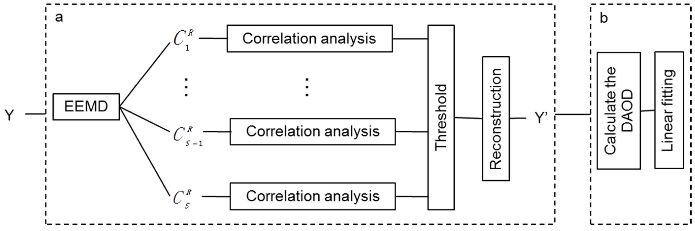
In the present study, we assume that the signals in a short time have the same useful information and that their differences are only caused by noise in stable atmospheric conditions. We apply the EEMD method to decompose the signals into different IMFs with frequencies ranging from high to low. Generally, we consider the noise existing in the high-frequency parts and implement signal de-noising by removing them. The correlation coefficients of the IMFs with the same temporal scale are regarded as the criterion to determine the components that need removal. Finally, we regard the linear fitting parameters of the differential absorption optical depth (DAOD) as the criterion for evaluating the de-noising effect.

In the next section, the system and theoretical foundation of the CO₂-DIAL and the EEMD method are presented in detail. Further, we study the feasibility of the method by processing simulated signals. Two parts were selected for the analysis, and an obvious improvement in the result was obtained. Moreover, we apply the above-mentioned method to the observed signal, and the r-square increased from 0.444 to 0.755, which is doubtless beneficial to the inversion precision. In conclusion, the method turns out to be applicable to simulated and observed signals.

2. Data and Methods

2.1. System and Theoretical Foundation of CO₂-DIAL

Our group is devoted to the development of a ground-based CO₂-DIAL system. The system located in Wuhan University involves four parts, namely, laser-emitting, frequency-stabilization, optical-receiving, and signal-acquisition systems. The system was designed to work at ~1.57 µm with a pulse repetition frequency of 20 Hz. Two close wavelengths were selected, and they were at the peak and wing of the absorption line, namely, on-wavelength (λ_on) and off-wavelength (λ_off), respectively. The sampling frequency is 20 MHz with a vertical range resolution of 7.5 m. The configuration of the lidar system is shown in the Figure 1.

The foundation of the CO₂-DIAL is the backscatter Lidar equation, as expressed in the following:

$$P_{on,off}(R)=\frac{P_{0}A\beta (R)\eta c\tau }{2R^2}·\exp (-2{\displaystyle \underset{0}{\overset{R}{\int }}(\alpha (R)+N{\sigma }_{on,off}(R))dr})$$

(1)

where R is the detection range, P is the received power of range R, P₀ is the transmitted power, A is the effective receiver area, c is the speed of light, τ is the laser pulse width, $\eta$ is the receiver efficiency, β(R) is the atmospheric backscatter coefficient, α(R) is the atmospheric extinction coefficient, N is the number density of CO₂, and σ is the absorption cross-section of CO₂. Because the on-line and off-line wavelengths are very close, β(R) and α(R) can be considered equivalent at two similar wavelengths. From Han et al., we can ignore the effect of water vapor through strict wavelength selection [15]. Given that the inversion of the CO₂ concentration is mainly based on the absorption difference of the on-line and off-line wavelength, a slight noise may cause a poor result. The signal intensity exponentially attenuates with range. Therefore, the amplitude of the signal affected by noise considerably varies at different ranges.

2.2. EEMD

The EMD proposed by Huang et al. is a non-linear, non-stationary, and self-adaptive decomposition technology that, unlike the traditional methods (Fourier transform, WT, etc.), dispenses with any basis functions and can decompose the signal into a series of IMFs.

$$y={\displaystyle \sum _{i=1}^n{c}_i}+r$$

(2)

where y is the signal, c_i represents the IMFs that include different frequency bands ranging from high to low, and r is the final residue that indicates the trend of the signal. Compared with previous methods, EMD requires no preliminary knowledge and possesses better adaptation. However, the method still suffers from the drawback of mode mixing, which makes the physical meaning of the IMFs unclear. To solve this problem, Wu and Huang [28] proposed a new NADA method named EEMD, which adds a white noise series with finite amplitude to the targeted data and then decomposes the data into IMFs. By repeating the above-mentioned process with different white noise series every time, we can obtain multiple IMFs with the same temporal scale. Ultimately, we treat the mean of the corresponding IMFs as the final result.

The EEMD algorithm can be directly defined by the following steps:

(1) Add random white noise n_i (t) with magnitude ε to the original signal s(t) to generate a new signal y_i(t) as

$$y_i(t)=s(t)+\epsilon n_i(t)$$

(3)

(2) Use the EMD method to decompose the new generated signal y_i(t) as

$$y_i(t)={\displaystyle \sum _{j=1}^m{c}_{i,j}}+r_{i,m}$$

(4)

(3) Calculate the mean of the corresponding IMFs and the residues as the final result as

$$c_j=\frac{1}{n}{\displaystyle \sum _{i=1}^n{c}_{i,j}}$$

(5)

and

$$r_m=\frac{1}{n}{\displaystyle \sum _{i=1}^n{r}_{i,m}}$$

(6)

where y_i(t) is the new generated signal, s(t) is the original signal, n_i(t) stands for different white noise series, c_i,j represents the IMFs, c_j is the mean of the corresponding IMFs of the decompositions, n is the ensemble number, r_i,m is the residue after n-times of decomposition, and r_m is the mean of the residues. By calculating the means of the IMFs and the residues, the added white noise series will finally cancel each other, and the problem of mode mixing can very well be solved.

As explained above, a series of IMFs with frequency ranging from high to low can be obtained. We generally consider the noise to exist in the high-frequency component. By removing the first few IMFs, we can achieve signal de-noising. Then, the key problem is how many IMFs should be removed.

In this work, we consider that the signals within a short time are similar to one another. In other words, the useful information in these signals is the same. Therefore, we simultaneously select several echo signals to decompose by EEMD and calculate the correlation coefficient of the IMFs with the same temporal scale. In the absence of the noise effect, the IMFs with the same temporal scale will have a strong correlation; otherwise, they have lesser relativity. According to the correlation coefficient, we can determine the number of removed IMFs.

The methodology shown in Figure 2 consists of two parts: signal de-noising and performance evaluation. The input matrix Y represents the original data, which includes three signal pairs. The first part starts by decomposing each segment into different time scales, $c_S^R$ (s = 1, 2, …, S), through EEMD and then calculating the correlation coefficient,$c_S^R$. Finally, the signal is reconstructed on the basis of the threshold. The second part mainly evaluates the de-noising performance by calculating the DAOD.

3. Simulated Signal Analysis

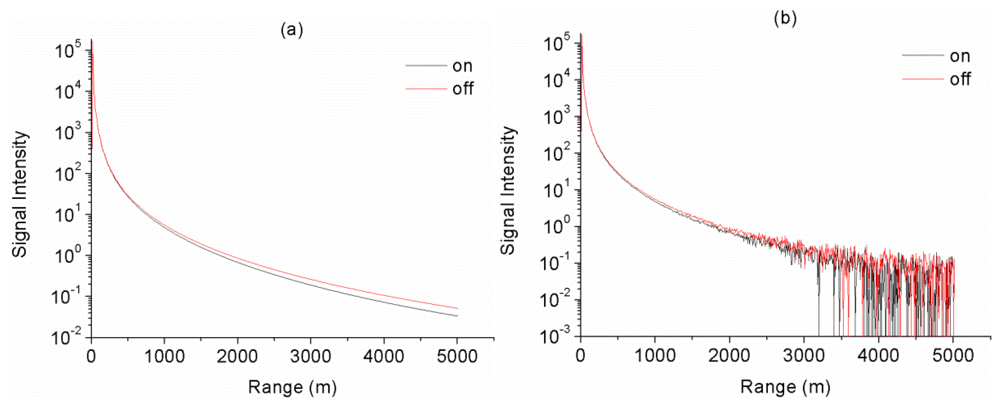
To verify the feasibility of the method, we analyzed the simulated CO₂-DIAL signal. Figure 3a shows the pure signal of the on-line and off-line wavelengths. The initial CO₂ concentration was assumed to be 400 parts per million, and the temperature and pressure profiles were obtained by interpolating the sounding data of the temperature and pressure at Wuhan in March 2015. Compared with the off-line wavelength, the on-line wavelength fell even more rapidly due to CO₂ absorption. We introduced a white noise into the simulated pure signal and considered their combination as the observed signal [Figure 3b]. Because of the influence of noise, the intensity of on-line wavelength echo signal may be stronger than off-line wavelength and can impair the absorption phenomenon. Thus, this problem can influence CO₂ retrieval precision. Hence, we introduced the above-mentioned method to process the echo signal.

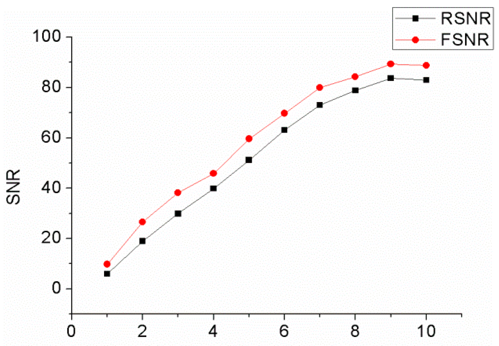
We proposed false SNR (FSNR) to approximately estimate the real SNR (RSNR) of the signal.

$$FSNR=10*\log \frac{{\displaystyle \sum _{t=1}^n{r}^2}}{{\displaystyle \sum _{T=1}^N{\left(C_1\right)}^2}}$$

(7)

and

$$RSNR=10*\log \frac{{\displaystyle \sum _{t=1}^n{S^2}_p}}{{\displaystyle \sum _{T=1}^N{\left(S_n-S_p\right)}^2}}$$

(8)

where r is final residue and can be viewed as useful information of the signal, C₁ is the first IMF and can approximately represent the noise of the signal, S_p and S_n represent the pure signal and noise of a signal, respectively. As Figure 4 shows, we have calculated the FSNRs and RSNRs of ten simulated signals. The difference between FSNR and RSNR is smaller, so we can substitute FSNR for RSNR.

FSNRs of ten measured signals have been calculated and they have minor difference between any two adjacent signals (

Table 1. The differences of FSNRs of measured signals.

Number	1	2	3	4	5	6	7	8
FSNR	97.198	96.637	98.711	96.151	97.165	98.817	99.130	99.419
Differences of FSNRs		0.561	2.074	2.560	1.014	1.653	0.313	0.289
Mean of the differences		1.209

). Therefore, three similar simulated signal groups with different SNRs, (99,100,101), were selected as our research objects (Figure 5). They can be considered as observed signals collected within a short time in stable atmospheric conditions. We segmented the signals into two parts to verify the performance of the method under different signal intensities. One part was approximately from 300 to 1500 m, and the other was from 1500 to 3000 m.

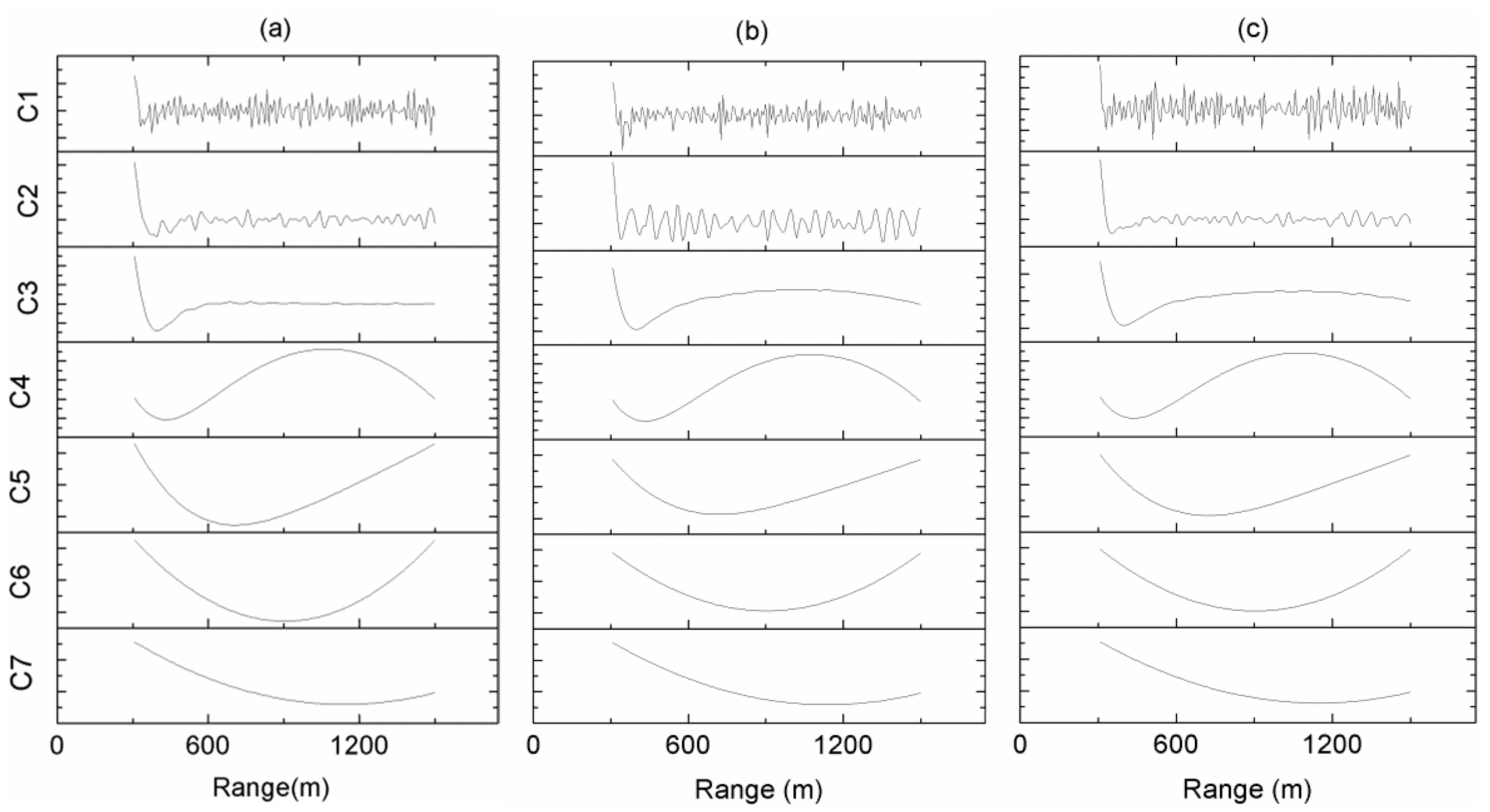
Figure 6 shows the IMFs of the selected simulated signals of the on-line wavelength from 300 to 1500 m decomposed by EEMD. The frequency of the IMF systematically decreased. We generally consider that IMFs with high frequency contain little useful information, and most of them are occupied by noise. Therefore, we assumed the IMFs with high frequency to be completely submerged in noise. We adopted the method of removing high-frequency IMFs to realize CO₂-DIAL signal de-noising. Therefore, the key to the problem was how to determine the IMFs that need to be removed. To solve this problem, the correlation coefficients of the IMFs with the same temporal scale were calculated.

We determined the IMFs that need to be removed and reconstructed the signal according to the following equations:

$$y_j={\displaystyle \sum _{s=1}^S{K}_s(t)C_{js}(t)}$$

(9)

and

$$K_s(t)=\{\begin{array}{ll}1& CR\ge 0.5\\ 0& CR<0.5\end{array}$$

(10)

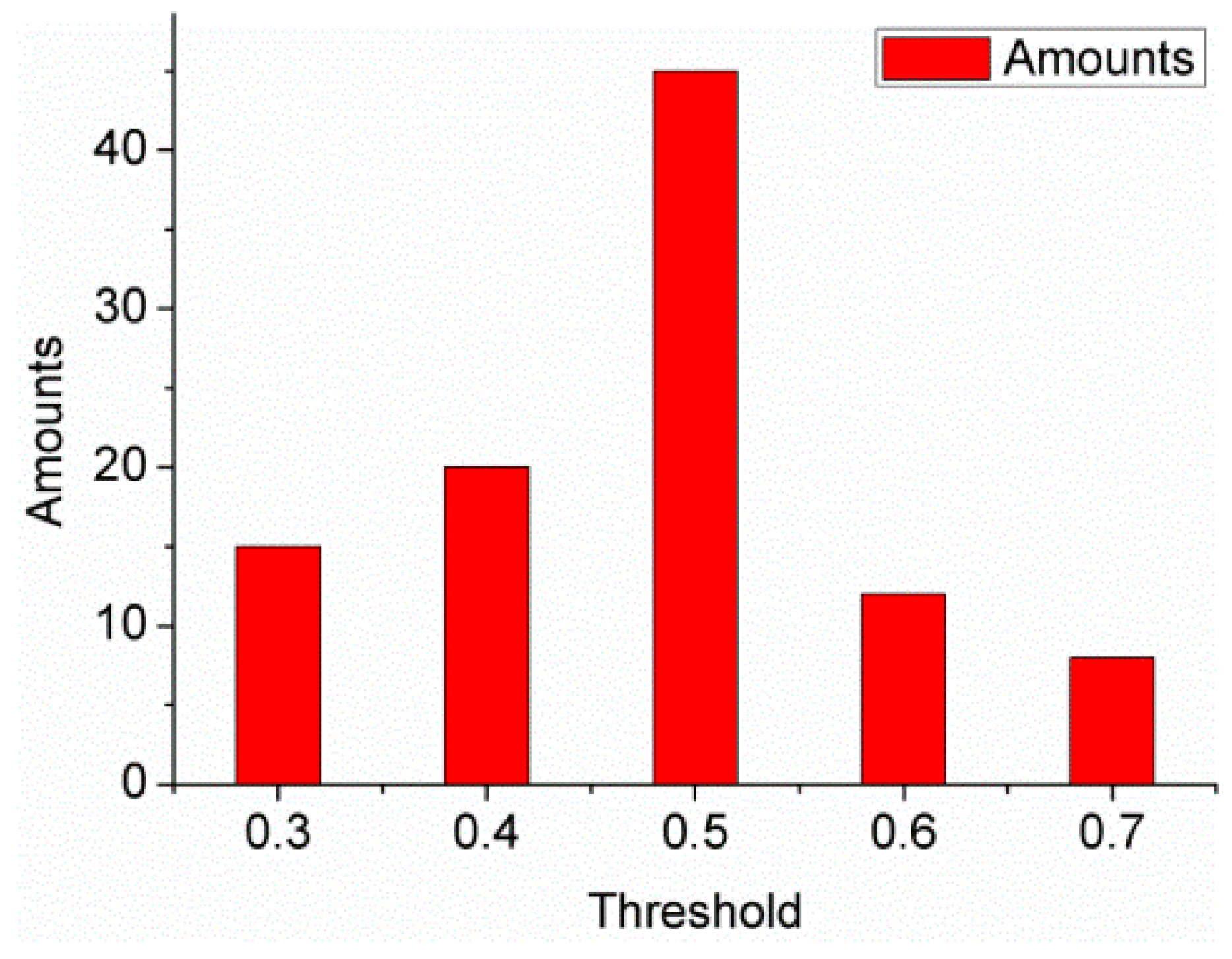
Signal y_j is reconstructed by several IMFs on individual scale C_js(t) (s = 1, 2, …, S) with a relevance factor K_s(t), where CR represents the correlation coefficients of the IMFs with the same temporal scale. We considered that the IMF contains more noise than useful information on the condition that half of all correlation coefficients are less than 0.5. The 0.5 correlation threshold is determined by a statistical experiment. The main idea of the experiment is to determine the threshold when the signal gets the maximum SNR and conduct a count in various thresholds. In order to verify the selection of threshold in various signal quality, we have simulated 50 signals with various SNR (51, 52, …, 100). We use the method proposed in this paper to analyze the signals in the sets of three and it totals 48 groups. The result showed that the signals obtained the maximum SNR when 0.3, 0.4, 0.6, 0.7 were selected as the criterion in some cases (Figure 7). Although sometimes several thresholds can also get the highest SNR, only the 0.5 correlation threshold can apply to almost all of the cases (45 groups in whole 48 groups). Therefore, a 0.5 correlation threshold is optimal.

The following table (

Table 2. Correlation coefficients of the IMFs with same temporal scale. (Left) On-line wavelength. (Right) Off-line wavelength.

C1				C1
λon	a	b	c	λoff	a	b	c
a	1.0000	−0.0595	−0.0254	a	1.0000	0.0235	0.0029
b	−0.0595	1.0000	−0.0443	b	0.0235	1.0000	−0.0579
c	−0.0254	−0.0443	1.0000	c	0.0029	−0.0579	1.0000
C2				C2
λon	a	b	c	λoff	a	b	c
a	1.0000	0.5718	0.5765	a	1.0000	0.6571	0.6984
b	0.5718	1.0000	0.7691	b	0.6571	1.0000	0.7428
c	0.5765	0.7691	1.0000	c	0.6984	0.7428	1.0000
C3				C3
λon	a	b	c	λoff	a	b	c
a	1.0000	0.9123	0.9709	a	1.0000	0.9206	0.9902
b	0.9123	1.0000	0.9710	b	0.9206	1.0000	0.9067
c	0.9709	0.9710	1.0000	c	0.9902	0.9067	1.0000
C4				C4
λon	a	b	c	λoff	a	b	c
a	1.0000	1.0000	0.9998	a	1.0000	0.9998	0.9998
b	1.0000	1.0000	0.9997	b	0.9998	1.0000	0.9992
c	0.9998	0.9997	1.0000	c	0.9998	0.9992	1.0000
C5				C5
λon	a	b	c	λoff	a	b	c
a	1.0000	0.9852	0.4979	a	1.0000	0.9609	0.4460
b	0.9852	1.0000	0.6376	b	0.9609	1.0000	0.6764
c	0.4979	0.6376	1.0000	c	0.4460	0.6764	1.0000
C6				C6
λon	a	b	c	λoff	a	b	c
a	1.0000	1.0000	1.0000	a	1.0000	1.0000	1.0000
b	1.0000	1.0000	1.0000	b	1.0000	1.0000	1.0000
c	1.0000	1.0000	1.0000	c	1.0000	1.0000	1.0000
C7				C7
λon	a	b	c	λoff	a	b	c
a	1.0000	0.9999	0.9997	a	1.0000	0.9998	1.0000
b	0.9999	1.0000	0.9993	b	0.9998	1.0000	0.9999
c	0.9997	0.9993	1.0000	c	1.0000	0.9999	1.0000

) lists the correlation coefficients of the IMFs with the same temporal scale of the on-line and off-line wavelengths. The correlation coefficients of the first IMF were comparatively low (i.e., below 0.5), whereas those of IMFs 2–7 reached more than 0.5. Therefore, we removed the first IMF and reconstructed the remaining components.

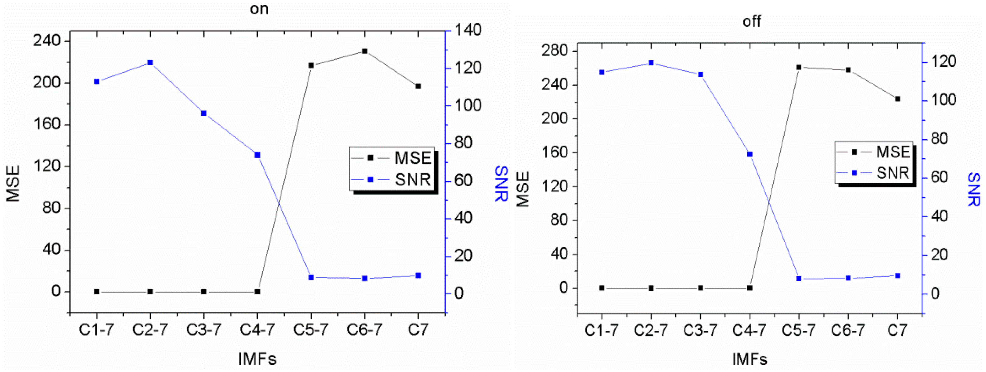
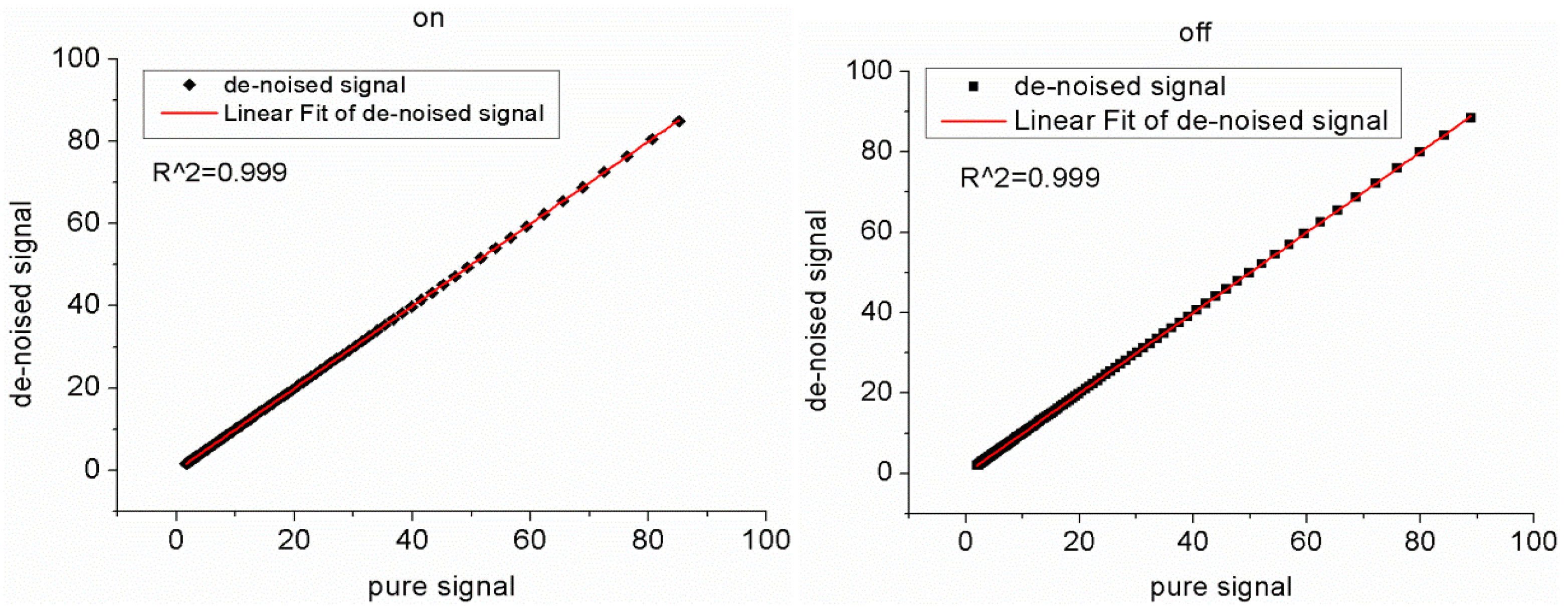
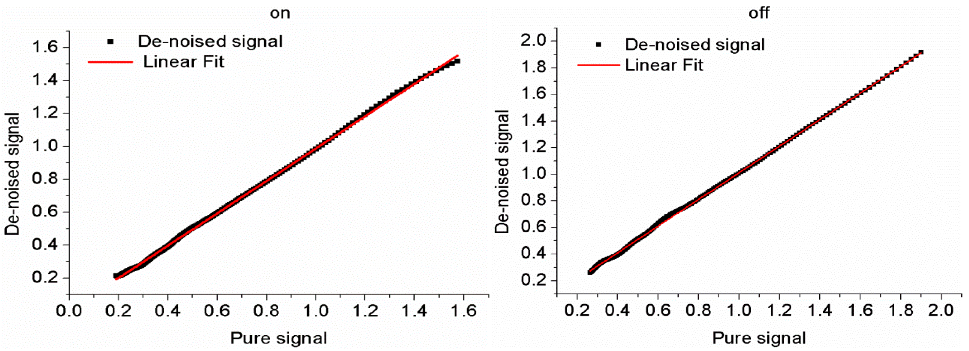
The ultimate purpose of de-noising is to improve the inversion accuracy; thus, we simultaneously analyzed the off-line wavelength.

Figure 8 shows the linear regression of the de-noised signal as a function of the pure signal. The good linear relationship demonstrates that the signals have a high degree of similarity. Meanwhile, the SNR and mean square error (MSE) were calculated (Figure 9). A better result was obtained after removing the first IMF.

From the above discussion, we can conclude that the method works well for on-line or off-line wavelength echo signals. However, evaluating the log ratio of two de-noised signals is more significant, which is crucial to the inversion precision. The following equation is the inversion formula for the CO₂ concentration [29,30]:

$$N_{CO2}=\frac{1}{2\left({\sigma }_{on}-{\sigma }_{off}\right)\Delta R}\ln \frac{P\left({\lambda }_{on},R_{bottom}\right)P\left({\lambda }_{off},R_{top}\right)}{P({\lambda }_{off},R_{bottom})P({\lambda }_{on},R_{top})}$$

(11)

where N_CO2 represents the concentration of CO₂, σ is the absorption cross-section of CO₂, and ΔR is the range resolution.

In this paper, DAOD refers to the difference between on-line and off-line wavelength in the CO₂-DIAL system, which is used to represent the difference between the two laser echo signals caused by CO₂ absorption. Then, Equation (11) can also be expressed as the following equation by DAOD:

$$N_{CO2}=\frac{DAOD}{2\left({\sigma }_{on}-{\sigma }_{off}\right)\Delta R}$$

(12)

Figure 10 shows the DAOD of the pure, original, and de-noised signal and directly shows that the data quality significantly improves and has a better fitting effect. The r-square listed in

Table 3. Linear fitting parameters of the DAOD for simulated signal from 300 to 1500 m.

	Pure	Original	De-Noised
R2	0.998	0.751	0.841
Slope	1.21 × 10−4	1.16 × 10−4	1.23 × 10−4

is consistent with this. According to Equation (12), the slope of the DAOD is the ratio of the DAOD and ΔR, which is important for the inversion of the CO₂ concentration. By comparing the slopes of the three data types, the slope of the de-noised signal is closer to the expected value, which demonstrates the validity of the de-noising method.

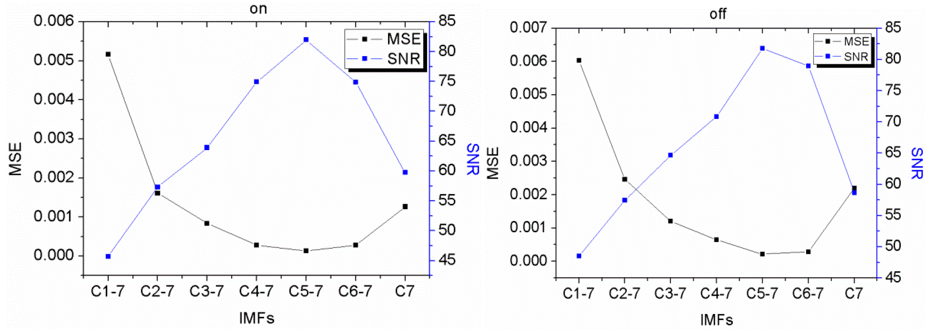
The above simulation results indicate that the method performed well in the range from 300 to 1500 m, which can be considered to have little noise influence. Further analysis should be implemented to assess the capability of the de-noising method. We performed the same steps specified above to analyze the range from 1500 to 3000 m, which is more readily affected by noise. Seven IMFs were obtained after EEMD, and we carried out signal reconstruction by removing the first four IMFs that did not meet the criteria (

Table 4. Linear fitting parameters of the DAOD for simulated signal from 1500 to 3000 m.

	Pure	Original	De-Noised
R2	0.997	0.027	0.835
Slope	8.88 × 10−5	1.11 × 10−4	9.25 × 10−5

). Compared with the pure signal, the de-noised signal had good consistency (Figure 11). Therefore, we can deduce that the de-noising process destroys little useful information from the original signal. The highest SNR and the lowest MSE were obtained when the first four IMFs were removed (Figure 12). These results suggest that the de-noising method works well for single signals.

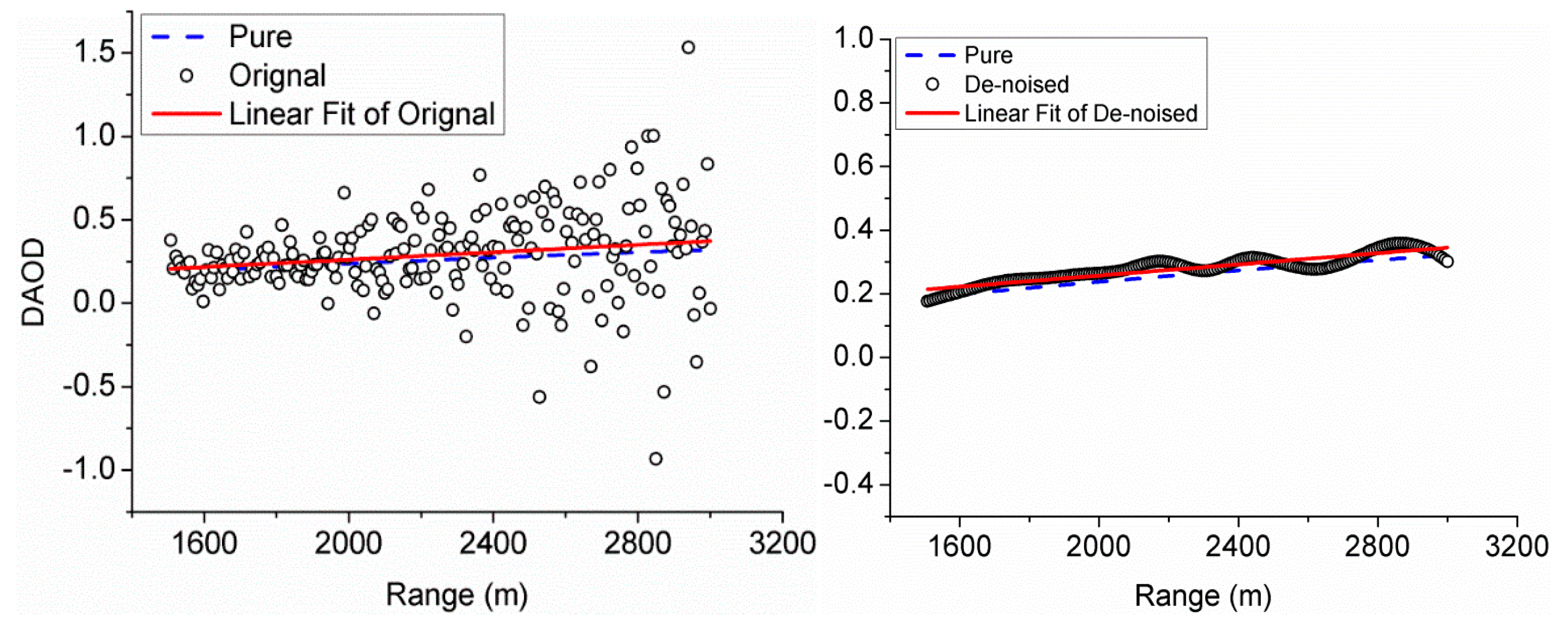
Because of the influence of noise, the signal intensity of the on-line and off-line wavelength signals was manifested; thus, the large changes in the log ratio of the two signals produced many negative values (Figure 13, left). These values impaired the validity and credibility of the linear fitting and led to a poor result. Nevertheless, a good result was obtained after implementing the de-noising method (Figure 13, right). The figure shows that no negative value was obtained, which fully illustrates that the errors of the two echo signals were greatly corrected. Because the DAOD represents the log ratio of two signals significantly smoothened after de-noising, some smooth fluctuations in the DAOD are acceptable. Moreover, the slope of the de-noised data was closer to the slope of the pure signal than that of the original signal (Table 4), which improved the inversion precision.

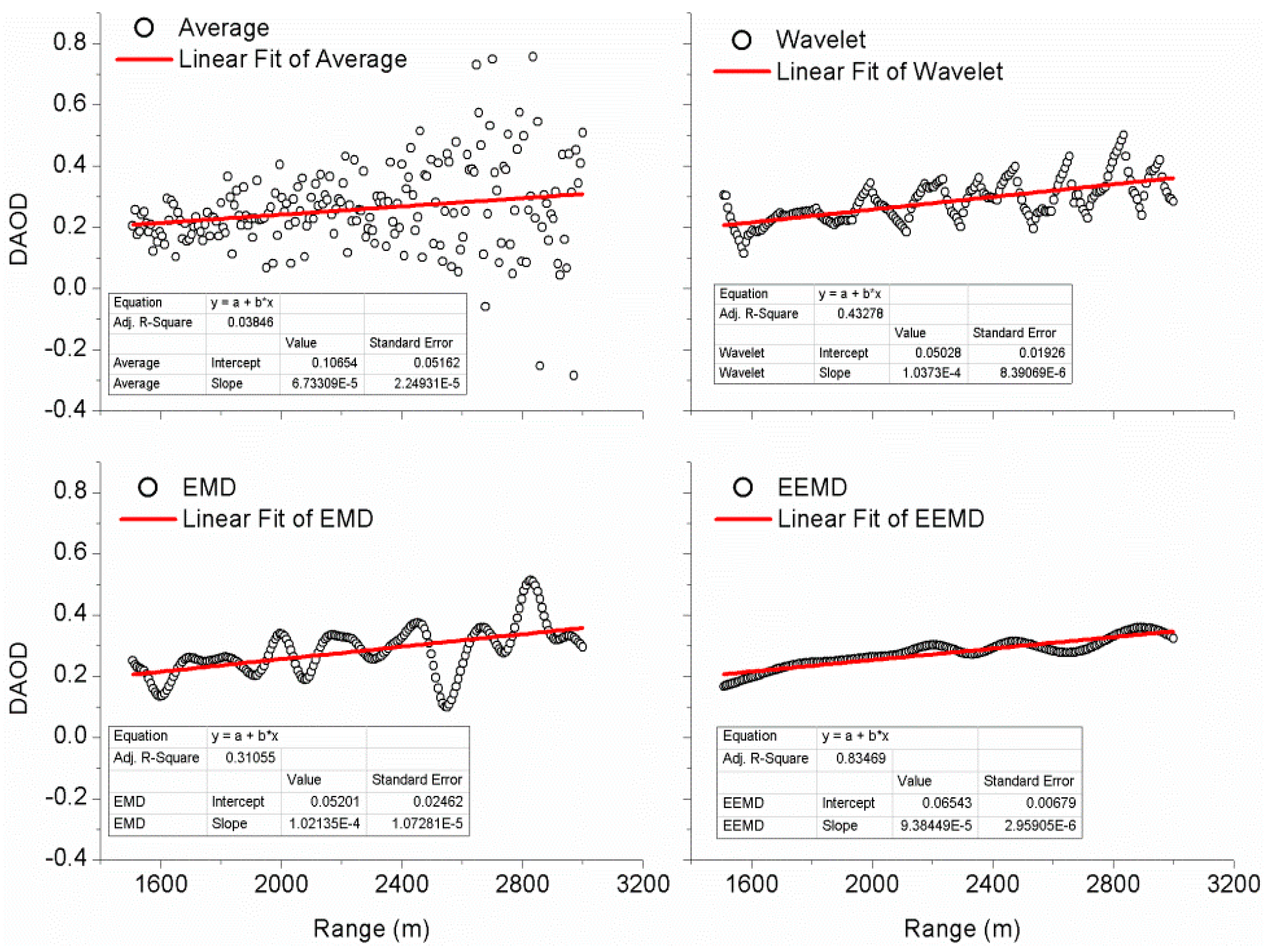
In order to further prove the superiority of the method in this paper, we compared the proposed method with several de-noising methods (Figure 14). The multi-pulse average method contributed little to the result. Compared with the EEMD method, the EMD and WT methods did not sufficiently improve the performance. From the data listed in

Table 5. Linear fitting parameters of the DAOD on the four de-noising methods.

	Average	Wavelet	EMD	EEMD
R2	0.028	0.433	0.311	0.835
Slope	6.01 × 10−5	1.04 × 10−4	1.02 × 10−4	9.25 × 10−5

, the EEMD method is more representative of the other methods.

4. Observed Signal Analysis

The CO₂-DIAL echo signal for analysis was collected in relatively stable atmospheric conditions and without acute changes on 29 December 2015. Thus, we assumed that the useful information of the signals is the same as one another; any difference could be due to the noise with a 30 s duration. Three signal pairs sequentially collected within 30 s were selected as our research objects; each pair includes on-line and off-line wavelength echo signals.

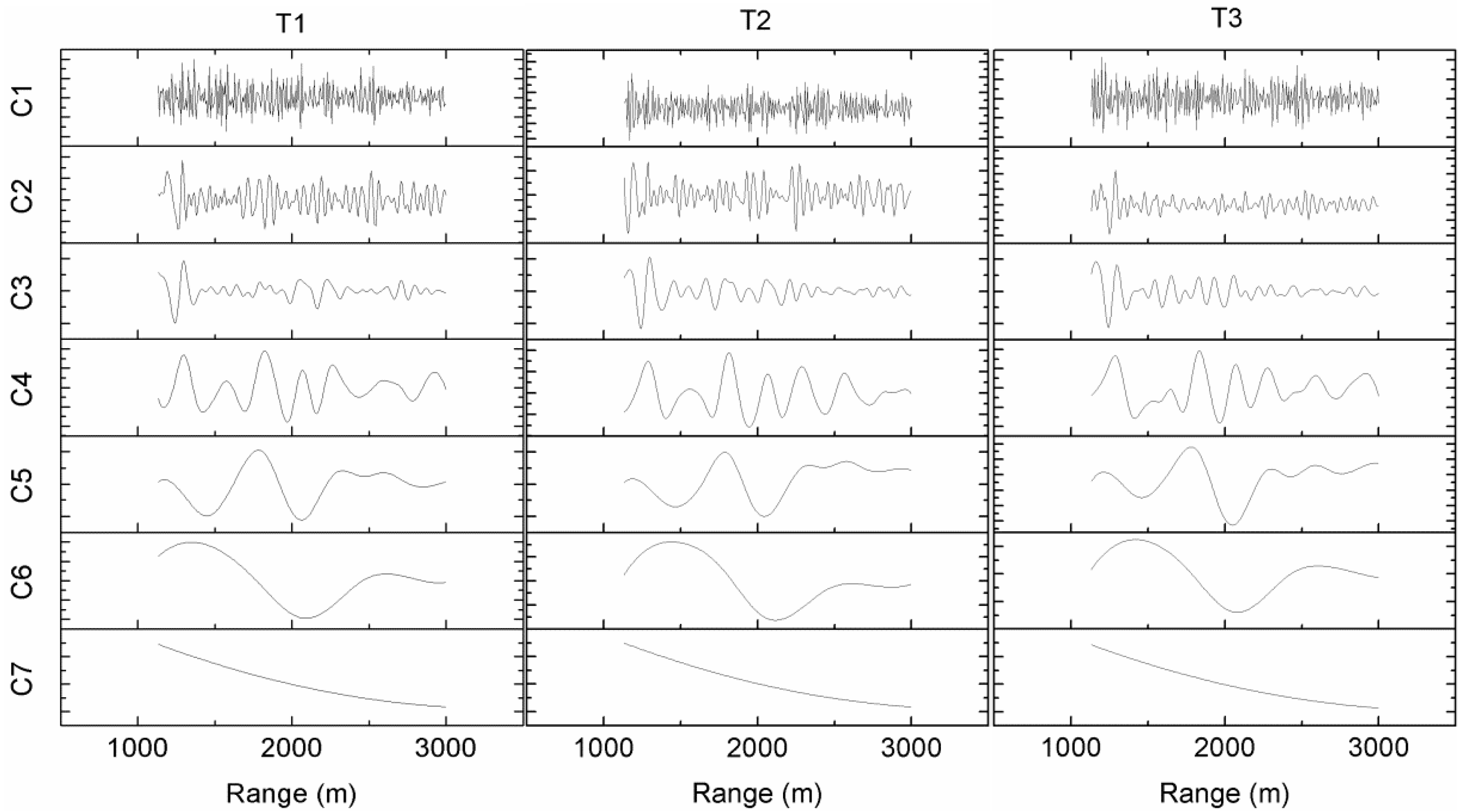
In our CO₂-DIAL system, two acquisition modes were used, namely, photon-counting and analog modes. The former has a better SNR, and the latter can compensate for the limitation in collecting the near-range echo signal of the former. Then, we chose the photonic signals of three signal pairs ranging from 1100 to 3000 m for presentation and named them as T1, T2, and T3. In particular, we only implemented signal de-noising on T2, and T1 and T3 served as reference signals. Figure 15 shows the IMFs of the off-wavelength echo signals of T1, T2, and T3. We calculated the correlation coefficients of the IMFs with the same temporal scale. From

Table 6. Correlation coefficients of the IMFs with the same temporal scale. (Left) On-line wavelength. (Right). Off-line wavelength.

C1				C1
λon	T1	T2	T3	λoff	T1	T2	T3
T1	1.0000	0.0634	0.1116	T1	1.0000	−0.0057	0.0464
T2	0.0634	1.0000	0.1003	T2	−0.0057	1.0000	−0.1694
T3	0.1116	0.1003	1.0000	T3	0.0464	−0.1694	1.0000
C2				C2
λon	T1	T2	T3	λoff	T1	T2	T3
T1	1.0000	0.2929	0.5217	T1	1.0000	0.2398	0.3347
T2	0.2929	1.0000	0.4128	T2	0.2398	1.0000	0.0155
T3	0.5217	0.4128	1.0000	T3	0.3347	0.0155	1.0000
C3				C3
λon	T1	T2	T3	λoff	T1	T2	T3
T1	1.0000	0.7089	0.7245	T1	1.0000	0.7922	0.7482
T2	0.7089	1.0000	0.7821	T2	0.7922	1.0000	0.8087
T3	0.7245	0.7821	1.0000	T3	0.7482	0.8087	1.0000

, we can find that the correlation coefficients of the first two IMFs are lower than 0.5. Those of the remaining IMFs that are not listed are higher than 0.5. Thus, we deleted the two IMFs and reconstructed the residue components.

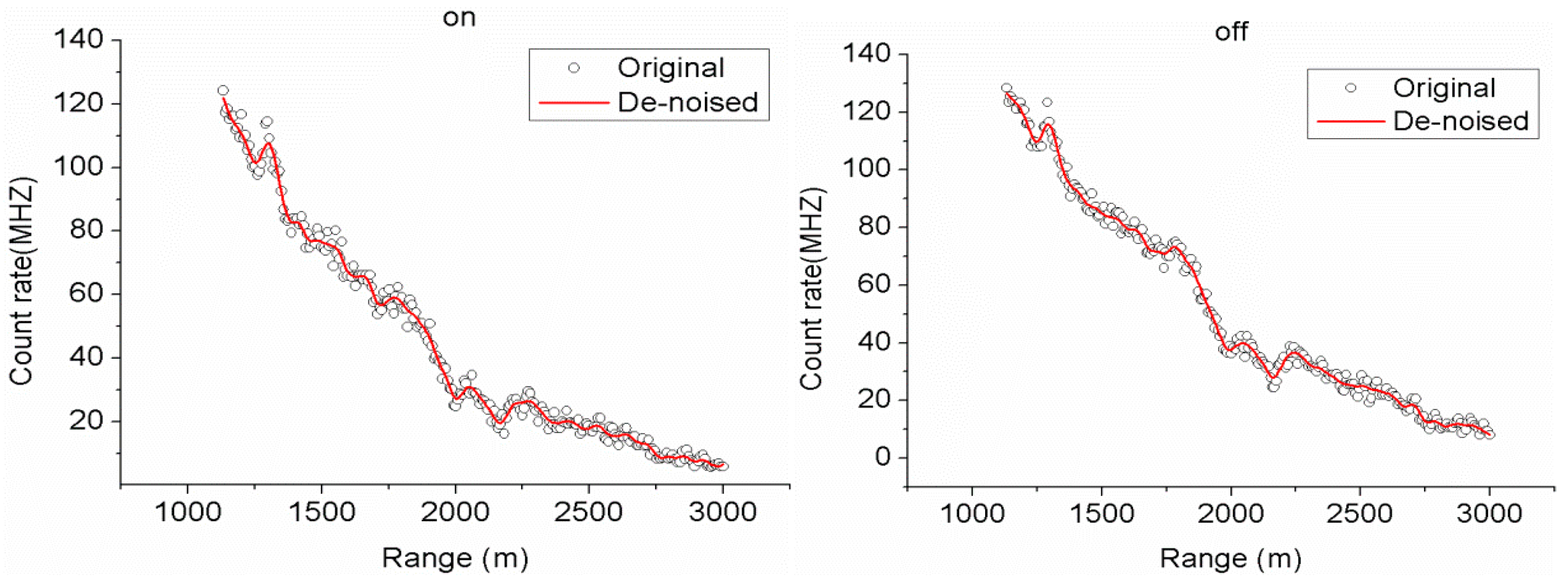
A good de-noising result is shown in the following (Figure 16). We see that the de-noising signal became smoother as well as retained the characteristics of the original signal. To validate the effect of the de-noising method for the investigated signal, we calculated the DAOD of the original and the de-noised signals. A significant improvement was obtained. The DAOD of the original signal showed negative values and had large discreteness (Figure 17). In contrast to the original signal, the de-noised signal had good linearity, and the r-square after linear fitting was 0.31 higher than that of the original signal (

Table 7. Linear fitting parameters of the DAOD for observed signal.

	Original	De-Noised
R2	0.444	0.755
Slope	1.83 × 10−4	1.77 × 10−4

). Moreover, the interference of the negative values was eliminated, which undoubtedly enhances the data reliability. Meanwhile, the slope of the DAOD improved to some extent.

5. Conclusions

For the CO₂-DIAL, CO₂ inversion is an important process. However, the existence of noise severely hinders the improvement of inversion precision. In this paper, we used the EEMD algorithm to de-noise the echo signals of the ground-based CO₂-DIAL system and set the threshold by calculating the correlation coefficients of the same scale components of multiple groups of adjacent signals decomposed by EEMD so as to determine the number of basic mode components to be removed. This method not only retains the useful information effectively but also removes the noise component. We decomposed three adjacent signal pairs into different IMFs using EEMD and removed the IMFs according to their correlation coefficients with the same temporal scale. Then, we reconstructed the residual components to complete the signal de-noising.

To verify the feasibility of the method, we analyzed the simulated CO₂-DIAL signal. Three similar simulated signal groups with different SNRs were selected as our research objects. They can be considered as observed signals collected within a short time in stable atmospheric conditions. We segmented the signals into two parts to verify the performance of the method under different signal intensities. First, the de-noised signal and the pure signal were compared in this paper. The good linear relationship between the de-noised signal and the pure signal demonstrates that the signals have a high degree of similarity. Meanwhile, the SNR and MSE were calculated to prove the effectiveness of the method proposed in this paper. Then, the DAOD of the de-noised signal is calculated. The R² of the DAOD reaches 0.841 and 0.835 for the detected range of 300–1500 m and 1500–3000 m, indicating that the quality is high, which is conducive to the high-precision inversion of CO₂. In order to further prove the superiority of the method in this paper, we also compared the proposed method with several de-noising methods. The results show that our method is more representative of the other methods in CO₂-DIAL de-noising. Finally, the method was used to observe CO₂-DIAL signal de-noising. The de-noised signal became smoother as well as retained the characteristics of the original signal. In contrast to the original signal, the de-noised signal had good linearity, and the R² of the DAOD was improved from 0.444 of the original signal to 0.735 of the de-noised signal, which is beneficial to the enhancement of the inversion precision. Certainly, this work may have some shortcomings. For example, the threshold for selecting the correlation coefficients was determined by many experiments but lacked theoretical foundations. We simply discussed the effect of the method under stable atmospheric conditions, and other cases were not considered. The above-mentioned deficiencies still require further research, and the proposed method requires continuous improvement in the future.

References

1. Stocker, T.F. Climate Change 2013: The Physical Science Basis: Working Group I Contribution to the Fifth Assessment Report of the Intergovernmental Panel on Climate Change; Cambridge University Press: Cambridge, UK, 2014. [Google Scholar]
2. Qiu, R.; Li, X.; Han, G.; Xiao, J.; Ma, X.; Gong, W. Monitoring drought impacts on crop productivity of the US Midwest with solar-induced fluorescence: GOSIF outperforms GOME-2 SIF and MODIS NDVI, EVI, and NIRv. Agric. For. Meteorol. 2022, 323, 109038. [Google Scholar] [CrossRef]
3. Rayner, P.; O’Brien, D. The utility of remotely sensed CO2 concentration data in surface source inversions. Geophys. Res. Lett. 2001, 28, 175–178. [Google Scholar] [CrossRef]
4. Gerbig, C.; Lin, J.; Wofsy, S.; Daube, B.; Andrews, A.; Stephens, B.; Bakwin, P.; Grainger, C. Toward constraining regional-scale fluxes of CO2 with atmospheric observations over a continent: 1. Observed spatial variability from airborne platforms. J. Geophys. Res. Atmos. 2003, 108, 4756. [Google Scholar]
5. Sawa, Y.; Matsueda, H.; Makino, Y.; Inoue, H.; Murayama, S.; Hirota, M.; Tsutsumi, Y.; Zaizen, Y.; Ikegami, M.; Okada, K. Aircraft Observation of CO2, CO, O3 and H2 over the North Pacific during the PACE-7 Campaign. Tellus B 2004, 56, 2–20. [Google Scholar] [CrossRef]
6. Stephens, B.B.; Gurney, K.R.; Tans, P.P.; Sweeney, C.; Peters, W.; Bruhwiler, L.; Ciais, P.; Ramonet, M.; Bousquet, P.; Nakazawa, T. Weak northern and strong tropical land carbon uptake from vertical profiles of atmospheric CO2. Science 2007, 316, 1732–1735. [Google Scholar] [CrossRef]
7. Abshire, B.; Riris, H.; Allan, G.R.; Weaver, C.; Mao, J.; Sun, X.; Hasselbrack, W.E.; Kawa, S.R.; Biraud, S. Pulsed airborne lidar measurements of atmospheric CO2 column absorption. Tellus B 2010, 62, 770–783. [Google Scholar] [CrossRef]
8. Abshire, B.; Riris, H.; Allan, G.R.; Weaver, C.; Mao, J.; Sun, X.; Hasselbrack, W.E.; Yu, A.; Amediek, A.; Choi, Y. A lidar approach to measure CO2 concentrations from space for the ASCENDS Mission. Proc. Spie. 2010, 7832, 289–301. [Google Scholar]
9. Pei, Z.; Han, G.; Ma, X.; Shi, T.; Gong, W. A Method for Estimating the Background Column Concentration of CO2 Using the Lagrangian Approach. IEEE Trans. Geosci. Remote Sens. 2022, 60, 1–12. [Google Scholar] [CrossRef]
10. Amediek, A.; Fix, A.; Ehret, G.; Caron, J.; Durand, Y. Airborne lidar reflectance measurements at 1.57 μm in support of the A-SCOPE mission for atmospheric CO2. Atmos. Meas. Techn. 2009, 2, 755–772. [Google Scholar] [CrossRef]
11. Ehret, G.; Kiemle, C.; Wirth, M.; Amediek, A.; Fix, A.; Houweling, S. Space-borne remote sensing of CO2, CH4, and N2O by integrated path differential absorption lidar: A sensitivity analysis. Appl. Phys. B 2008, 90, 593–608. [Google Scholar] [CrossRef]
12. Sakaizawa, D.; Nagasawa, C.; Nagai, T.; Abo, M.; Shibata, Y.; Nakazato, M.; Sakai, T. Development of a 1.6 μm differential absorption lidar with a quasi-phase-matching optical parametric oscillator and photon-counting detector for the vertical CO2 profile. Appl. Opt. 2009, 48, 748–757. [Google Scholar] [CrossRef] [PubMed]
13. Kameyama, S.; Imaki, M.; Hirano, Y.; Ueno, S.; Kawakami, S.; Nakajima, M. Development of 1.6 micron CW modulation ground-based DIAL system for CO2 monitoring. Asia-Pac. Remote Sens. Int. Soc. Opt. Photonics 2008, 7153, 71530L. [Google Scholar]
14. Riris, H.; Burris, J.; Krainak, M.; Sun, X.; Abshire, J. A 1.57 µm DIAL Lidar System for Range Resolved Measurements of Atmospheric CO2. In Proceedings of the Conference on Lasers and Electro-Optics, (Optical Society of America 2006), Long Beach, CA, USA, 21–26 May 2006; p. ThC82. [Google Scholar]
15. Han, G.; Gong, W.; Lin, H.; Ma, X.; Xiang, Z. Study on Influences of Atmospheric Factors on Vertical Profile Retrieving from Ground-Based DIAL at 1.6 μm. Geosci. Remote Sens. IEEE Trans. 2015, 53, 3221–3234. [Google Scholar] [CrossRef]
16. Reba, M.N.M.; Rocadenbosch, F.; Sicard, M. A straightforward signal-to-noise ratio estimator for elastic/Raman lidar signals. Remote Sens. Int. Soc. Opt. Photonics 2006, 6362, 636223.1–636223.12. [Google Scholar]
17. Rocadenbosch, F.; Comerón, A.; Pineda, D. Assessment of lidar inversion errors for homogeneous atmospheres. Appl. Opt. 1998, 37, 2199–2206. [Google Scholar] [CrossRef]
18. Dragomiretskiy, K.; Zosso, D. Variational Mode Decomposition. IEEE Trans. Signal Process. 2014, 62, 531–544. [Google Scholar] [CrossRef]
19. Li, M.; Jiang, L.H.; Xiong, X.L. A novel EMD selecting thresholding method based on multiple iteration for denoising LIDAR signal. Opt. Rev. 2015, 22, 477–482. [Google Scholar] [CrossRef]
20. Li, H.; Chang, J.; Xu, F.; Liu, Z.; Yang, Z.; Zhang, L.; Zhang, S.; Mao, R.; Dou, X.; Liu, B. Efficient Lidar Signal Denoising Algorithm Using Variational Mode Decomposition Combined with a Whale Optimization Algorithm. Remote Sens. 2019, 11, 126. [Google Scholar] [CrossRef]
21. Dai, H.; Gao, C.; Lin, Z.; Wang, K.; Zhang, X. Wind lidar signal denoising method based on singular value decomposition and variational mode decomposition. Appl. Opt. 2021, 60, 10721–10726. [Google Scholar] [CrossRef]
22. Zhou, Z.; Hua, D.; Wang, Y.; Yan, Q.; Li, S.; Li, Y.; Wang, H. Improvement of the signal to noise ratio of Lidar echo signal based on wavelet de-noising technique. Opt. Lasers Eng. 2013, 51, 961–966. [Google Scholar] [CrossRef]
23. Mao, F.; Gong, W.; Li, C. Anti-noise algorithm of lidar data retrieval by combining the ensemble Kalman filter and the Fernald method. Opt. Express 2013, 21, 8286–8297. [Google Scholar] [CrossRef] [PubMed]
24. Wu, S.; Liu, Z.; Liu, B. Enhancement of lidar backscatters signal-to-noise ratio using empirical mode decomposition method. Opt. Commun. 2006, 267, 137–144. [Google Scholar] [CrossRef]
25. Tian, P.; Cao, X.; Liang, J.; Zhang, L.; Yi, N.; Wang, L.; Cheng, X. Improved empirical mode decomposition based denoising method for lidar signals. Opt. Commun. 2014, 325, 54–59. [Google Scholar] [CrossRef]
26. Huang, N.E.; Shen, Z.; Long, S.R.; Wu, M.C.; Shih, H.H.; Zheng, Q.; Yen, N.-C.; Tung, C.C.; Liu, H.H. The empirical mode decomposition and the Hilbert spectrum for nonlinear and non-stationary time series analysis. Proc. R. Soc. Lond. A Math. Phys. Eng. Sci. 1998, 454, 903–995. [Google Scholar] [CrossRef]
27. Wu, Z.; Huang, N.E. A study of the characteristics of white noise using the empirical mode decomposition method. Proc. R. Soc. Lond. A Math. Phys. Eng. Sci. 2004, 460, 1597–1611. [Google Scholar] [CrossRef]
28. Wu, Z.; Huang, N.E. Ensemble empirical mode decomposition: A noise-assisted data analysis method. Adv. Adapt. Data Anal. 2009, 1, 1–41. [Google Scholar] [CrossRef]
29. Shi, T.; Han, G.; Ma, X.; Gong, W.; Chen, W.; Liu, J.; Zhang, X.; Pei, Z.; Gou, H.; Bu, L. Quantifying CO2 uptakes over oceans using LIDAR: A tentative experiment in Bohai bay. Geophys. Res. Lett. 2021, 48, e2020GL091160. [Google Scholar] [CrossRef]
30. Shi, T.; Han, G.; Ma, X.; Zhang, M.; Pei, Z.; Xu, H.; Qiu, R.; Zhang, H.; Gong, W. An inversion method for estimating strong point carbon dioxide emissions using a differential absorption Lidar. J. Clean. Prod. 2020, 271, 122434. [Google Scholar] [CrossRef]
Figure 1. Configurations of ground-based CO2-DIAL system.
Atmosphere 13 01361 g001
Figure 2. Methodology of the CO2-DIAL signal de-noising: (a) shows the signal de-noising by EEMD, and (b) shows the performance evaluation.
Atmosphere 13 01361 g002
Figure 3. Simulated CO2−DIAL signal. (a) Pure signal of the on−line and off−line wavelengths. (b) Signal with white noise.
Atmosphere 13 01361 g003
Figure 4. FSNR and RSNR of simulated signals.
Atmosphere 13 01361 g004
Figure 5. Similar simulated signals, which can be considered as measured signal collected within a short time: (a) previous time of the signal that needs de−noising; (b) signal that needs de−noising, and (c) following time of signal that needs de−noising.
Atmosphere 13 01361 g005
Figure 6. IMFs of the three selected simulated signals of the on-line wavelength. (a) IMFs of the signal at previous time; (b) IMFs of the signal at a certain time, and (c) IMFs of the signal at following time.
Atmosphere 13 01361 g006
Figure 7. Number of groups getting the highest SNR at different thresholds.
Atmosphere 13 01361 g007
Figure 8. Comparison between the de-noised and pure signals. (Left) On-line wavelength. (Right) Off-line wavelength (the de-noised signal is reconstructed by IMFs 2–7).
Atmosphere 13 01361 g008
Figure 9. SNR and MSE of the de-noised signal. (Left) On–line wavelength. (Right) Off-line wavelength. The x-axis label indicates the sum of the IMFs and C represents IMF. For example, the first is the sum of IMFs 1–7, the second is the sum of IMFs 2–7, and the last is IMF 7.
Atmosphere 13 01361 g009
Figure 10. Comparison of the DAOD from 300 to 1500 m. (Left) Pure and original signal. (Right) Pure and de-noised signal.
Atmosphere 13 01361 g010
Figure 11. Comparison between the de-noised and pure signals. (Left) On-line wavelength. (Right) Off-line wavelength. The de-noised signal is reconstructed by IMFs 5–7.
Atmosphere 13 01361 g011
Figure 12. (Right axis) SNR and (left axis) MSE of the de-noised signals. (Left) On-line wavelength. (Right) Off-line wavelength.
Atmosphere 13 01361 g012
Figure 13. Comparison of the DAOD from 1500 to 3000 m. (Left) Pure and original signal. (Right) Pure and de−noised signal.
Atmosphere 13 01361 g013
Figure 14. Comparison of the four de-noising methods. (Upper left) Multi−pulse average method. (Top right) Wavelet de−noising method. (Left bottom) EMD. (Lower right) Proposed method (EEMD) in this paper.
Atmosphere 13 01361 g014
Figure 15. IMFs of the off-wavelength echo signals of T1, T2, and T3 (C1, C2, …, C7 represent various temporal scales).
Atmosphere 13 01361 g015
Figure 16. Comparison of the original and de-noised signals. (Left) On-line wavelength. (Right) Off-line wavelength.
Atmosphere 13 01361 g016
Figure 17. Comparison of the DAOD of the original and de−noised signals from 1100 to 3000 m. (Left) Original signal. (Right) De−noised signal.
Atmosphere 13 01361 g017