Preliminary Application of a Multi-Physical Ensemble Transform Kalman Filter in Cloud and Precipitation Forecasts

Abstract

In this study, based on the retrieval data from the Fengyun geostationary meteorological satellite and the Tropical Rainfall Measuring Mission satellite, a large-scale precipitation case in eastern China is selected to address the systematic deviations of deterministic forecasts for clouds and precipitation. A multi-physical ensemble transform Kalman filter (ETKF) is constructed in this research based on the Weather Research and Forecast model version 3.6, and its forecasting ability in terms of cloud-top height and temperature, hydrometeors, and precipitation is evaluated by quantitatively comparing three microphysical parameterization schemes (Lin, Morrison, and CAM5.1 schemes) and their corresponding multi-physical ensemble mean. The results show that the Lin, Morrison, and CAM5.1 schemes all underestimate the range of cloud systems and have different advantages and disadvantages in forecasting different elements, while the forecasting improvement of the multi-physical ensemble mean is limited. However, the multi-physical ETKF can effectively improve the forecast accuracy of the cloud system range. In addition, the multi-physical ETKF has the advantages of different physical parameterization schemes, which can dramatically improve the forecast accuracy of cloud hydrometeors, reduce precipitation forecast errors, and improve threat scores.

1. Introduction

Weather modification in China has become an essential basic public welfare undertaking for the coordinated development of state and local governments after years of development [1,2,3]. Many studies have shown that a successful weather modification operation is inseparable from a comprehensive understanding of the cloud features [4,5,6,7]. Therefore, the accurate forecast of cloud features in the atmosphere is the key to the efficient development of cloud water resources and artificial rainfall.

As an open-source advanced mesoscale numerical model, the WRF model provides many physical parameterization schemes and can accurately simulate mesoscale weather processes [8,9]. Therefore, the WRF model is feasible for simulating cloud features [10,11,12]. However, there are some deviations in the simulation results [13,14]. Numerous studies have shown that microphysical parameterization schemes in the WRF model can greatly influence the simulation’s performance [15,16,17]. Cintineo et al. [18] compared four double-moment microphysics schemes and found that the forecast performances of the schemes are quite different for different cloud particles; for example, the Thompson scheme can accurately forecast the upper-level clouds, and the Morrison scheme performs well in the forecast of low-level clouds. Pu et al. [19] found that in the southern plain areas of the US, the Morrison scheme performs well in forecasting convective precipitation, but Huang et al. [20] pointed out that this conclusion does not apply in the coastal areas of China. Therefore, the selection of microphysical parameterization schemes is complex and has many uncertainties.

In order to solve the above simulation bias, this study attempts to construct a multi-physical ensemble transform Kalman filter (ETKF), which considers not only the uncertainty of the initial values [21,22,23,24,25,26,27] but also the effect of different microphysical parameterization schemes on simulations. The ensemble transform Kalman filter (ETKF) is a widely used initial perturbation method at present, which was first proposed by Bishop et al. [28] in adaptive observation and can directly estimate the prediction error covariance matrix associated with a particular deployment of observational resources. Further, Peffers [29] pointed out that the multi-physical ETKF can effectively conduct initial perturbation and obtain a more reasonable ensemble spread and Taylor distribution than a single-physics process. Zhang et al. [30] also verified that introducing multi-physical parameterization and multi-boundary perturbation schemes could greatly improve the quality of ensemble members and the precipitation forecasts. Huang et al. [31] conducted a similar study and demonstrated the advantages of the multi-physical ETKF, especially in improving rainstorm forecasts. The above studies show that multi-physical and multi-initial values can greatly improve the ensemble dispersion and thus improve the forecast performance. It is also necessary to discuss whether the multi-physical ETKF can also improve cloud water forecasts. Therefore, taking a large-scale precipitation process in the summer of 2014 as a study case, we first evaluate different microphysical parameterization schemes and then compare the improvement of the multi-physical ensemble mean (hereinafter referred to as Multi-Physical) and multi-physical ETKF (hereinafter referred to as ETKF) in cloud water forecasts.

2. Data and Methods

2.1. Model and Observations

The WRF (Advanced Research WRF) version 3.6 is used in this study to simulate a large-scale precipitation case in eastern China during the summer of 2014. The National Centers for Environmental Prediction-Final Operational Global Analysis (NCEP/FNL) data with a resolution of 1° × 1° is chosen as the initial and boundary conditions [32]. The starting time of this forecast is 0000 UTC on August 12, 2014, the forecast lead time is 48 hours, and the output interval is 3 hours. Thus, a total of 16 sets of sample data are outputted. The integration time step is 60 s, and the horizontal resolution is 15 km. The model adopts a single domain without a nest, with 45 vertical layers. The simulated area is the range of 25° N–40° N, 105° E–125° E (Figure 1). In this study, three microphysical parameterization schemes, i.e., Lin [33], Morrison [34], and Community Atmosphere Model (CAM5.1) [35], are selected for comparative tests. Other parameterization schemes used in the experiments are the Monin–Obukhov surface layer scheme [36], rapid radiative transfer model long-wave radiation scheme [37], Dudhia short-wave radiation scheme [38], Noah land surface process scheme [39], and Yonsei University planetary boundary layer scheme [40].

In this study, the cloud-top height, cloud-top temperature, and hydrometeors are not directly outputted by the WRF, which needs to be calculated according to the outputs. The specific calculation methods are as follows: the maximum height where the SUM (Equation (1)) is greater than the threshold value (the selection of the threshold value is discussed in detail below) is defined as the cloud-top height, and the temperature corresponding to the cloud-top height is defined as the cloud-top temperature. The hydrometeors are obtained by Equations (2)–(4).

$$\mathrm{SUM}=qc+qr+qi+qs+qg+qh$$

(1)

$$\mathrm{CWP}=\frac{1}{g}{{\displaystyle \int }}_{pbot}^{ptop}qc\left(p\right)dp$$

(2)

$$\mathrm{RWP}=\frac{1}{g}{{\displaystyle \int }}_{pbot}^{ptop}qr\left(p\right)dp$$

(3)

$$\mathrm{IWP}=\frac{1}{g}{{\displaystyle \int }}_{pbot}^{ptop}\left(qi\left(p\right)+qs\left(p\right)+qg\left(p\right)+qh\left(p\right)\right)dp$$

(4)

qc, qr, qi, qs, qg and qh indicate the mass concentration ratios (kg∙kg⁻¹) of cloud water, rainwater, ice crystals, snow crystals, graupel, and hail, respectively, and pbot and ptop represent the bottom and top air pressure (hPa), g the acceleration of gravity (m∙s⁻²).

The retrieval product from Fengyun geostationary meteorological satellite is used as the observation data of the cloud macrophysical variables. This data is obtained from the joint retrieval of detection data from the Fengyun geostationary meteorological satellite and L-band second-level sounding data, with a resolution of 0.05° × 0.05°. In this study, the cloud-top height and temperature retrieved based on this data are selected as the observation data for the quantitative verification.

The hydrometeor retrieval data from the Tropical Rainfall Measuring Mission version 7 (TRMM 2A12 product) is also used as the observation data of the hydrometeors. Compared with the TRMM version 6, the number of vertical layers in TRMM version 7 is increased from 14 to 28. Moreover, the layer depth is 0.5 km for the height below 10 km and 1 km for the height above 10 km, making the description of vertical features more accurate. Since the TRMM satellite orbits the earth about 16 times every day, the on-orbit data obtained as the TRMM satellite passes through the study area are selected in this study. The retrieved CWP, RWP, and IWP are used as the observation data for the quantitative verification.

The precipitation retrieval data adopt the fusion product of the automatic weather station network observations of the China Meteorological Administration and the Climate Prediction Center morphing technique (CMORPH) data [41] with a spatio-temporal resolution of 1 hour and 0.1° × 0.1°. Among them, the automatic weather station observations are the hourly precipitation from 30,000–40,000 automatic weather stations in China with quality control, and the CMORPH satellite precipitation product is from the Climate Prediction Center of the National Oceanic and Atmospheric Administration, with a spatio-temporal resolution of 30 minutes and 8 km × 8 km.

2.2. The Microphysical Parameterization Schemes

Lin’s scheme [33] is a relatively mature single-moment microphysics scheme in the WRF model relating to various cloud particles. This scheme provides the specific water contents of cloud water, rainwater, ice crystal, snow, and graupel. Moreover, physical processes, such as the mutual transformation of ice crystals and cloud water and the collision and phase change of different particles, are considered. It is suitable for high-resolution simulations.

The Morrison 2-mom scheme [34] is a double-moment microphysics scheme relating to many types of particles, such as cloud water, rainwater, ice crystals, snow, graupel, and water vapor. In addition to cloud particles, mixing ratios and number concentrations of other particles are predicted. This scheme contains more than 40 kinds of cloud physical processes, which can describe the cloud physical processes accurately and comprehensively.

The CAM5.1 scheme [35] is a double-moment microphysics scheme relating to several particles of cloud water, rainwater, ice crystals, and snow, which can simulate the mixing ratios and number concentrations of all particles. The scheme was ported from the CAM5 model into the WRF model in 2013, with relatively complex physical processes.

2.3. The Multi-Physical and the Multi-Physical ETKF Schemes

This study mainly performs multi-physical ensemble mean on three microphysical schemes, i.e., Lin’s, Morrison’s, and CAM5.1 schemes. The calculation formula of the Multi-Physical is as follows (Equation (5)). The experimental design is shown in

Table 1. Experiment design for two ensemble methods.

Experiment	Number of Ensemble Members	Initial Perturbations	Microphysical Schemes
Multi-Physical	3	NO	Member 1 adopts Lin’s, Member 2 adopts Morrison’s, Member 3 adopts CAM5.1
multi-physical ETKF	15	Generate 15 perturbations	Member 1–5 adopt Lin’s, Member 6–10 adopt Morrison’s Member 11–15 adopt CAM5.1

.

$$\mathrm{EMN}=\frac{1}{N}{\displaystyle \sum }_{i=1}^N{F}_i$$

(5)

where $F_i$ represents the predicted value of the ith microphysical parameterization scheme, and N denotes the total number of schemes.

In this study, the ETKF method is used to construct initial perturbations of the ensemble. This method assumes that the forecast perturbation covariance is the same as the forecast error covariance. Therefore, the Kalman filter is expressed as follows (Equations (6) and (7)).

$$P^a=Z^a\left(Z^a\right){}^T$$

(6)

$$P^f=Z^f\left(Z^f\right){}^T$$

(7)

where $P^a$ indicates the analysis error covariance, $Z^a$ the analysis perturbation, $P^f$ the forecast error covariance, and $Z^f$ the predicted perturbation. When the data assimilation system performs better, the forecast error covariance ($P^f$) and the analysis error covariance ($P^a$) satisfy the update equation of Kalman filter error covariance (Equation (8)).

$$P^a=P^f-P^f{H}^T(H{P}^f{H}^T+R){}^{-1}H{P}^f$$

(8)

where R denotes the observation error covariance matrix, R for this experiment is the default one in WRFDA, and H represents the linearized observation operator that converts the predicted value from the grid point to the observation station. Subsequently, a transformation matrix T is introduced, which can be calculated by converting the predicted perturbation into an analysis perturbation. In this way, based on the ETKF method, the analysis perturbation is obtained by multiplying the predicted perturbation by a transformation matrix T. In this study, the perturbations of different parameterization schemes are considered based on the ETKF, and the specific steps are as follows.

First, the NCEP/FNL data at 0000 UTC on 8 August 2014, is selected as the initial field of the model. A set of small perturbations (15) is randomly generated by the Monte Carlo method and superimposed on the analysis field of zonal wind, meridional wind, potential temperature, water vapor, and geopotential height to obtain 15 random initial perturbation fields of the WRF model at that moment.

Then, the generated 15 initial perturbations are divided into 3 groups, and each group (5 random perturbations) corresponds to different microphysical parameterization schemes of the CAM5.1, Morrison 2-mom, and Lin.

Subsequently, the above 15 initial perturbations are input into the WRF model for 12-hour integration to obtain the forecast field at 1200 UTC on August 8. The forecast perturbations at that moment are obtained by subtracting the forecast results of the 15 ensemble members from the mean of these forecast results. The transformation matrix and amplification factor are calculated by the Kalman filter formula, and then the new analysis perturbations at 1200 UTC on August 8 can be obtained by the ETKF method. Superimposing these 15 analysis perturbations onto the WRF analysis field at 1200 UTC on August 8, we obtain 15 initial perturbation fields at that moment and use the lateral boundary update in the WRF data assimilation system to update the boundary field. Repeat the above steps. After a 4-day cycle, the amplification factor changes less and tends to be stable at 0000 UTC on August 12. Next, the forecast results obtained by a 48-hour integration are verified.

2.4. Quantitative Evaluations

In order to facilitate quantitative verification, the resolutions of the model data and the observation data should be consistent. Therefore, the model data are interpolated by the bilinear interpolation method. The quantitative evaluations of the Multi-Physical and multi-physical ETKF are based on the ensemble mean of their respective ensemble members. The calculation of the ensemble mean at a specific grid point obeys the following rule: the results can be calculated only when more than half of the members simulate the presence of clouds; otherwise, it is regarded as no cloud at this point. Due to the inconsistent forecast capabilities of different schemes in different regions, the region of 25° N–35° N, 107° E–123° E is selected as the area of evaluation. Anomaly correlation coefficient (ACC) and root mean square error (RMSE) are two commonly used statistics (Equations (9) and (10)), which can directly reflect the forecast effect and errors of the model. The ACC indicates the correspondence between the forecast results and the observations and reflects the deviation of the forecast. The closer the ACC is to 1, the closer the forecast results are to the observations. Threat score (TS) is a commonly used and effective index for meteorological research to evaluate precipitation forecasts. The TS has a variety of expressions, while this study uses a grid-to-grid method to evaluate the simulated precipitation (Equation (11)).

$$\mathrm{ACC}=\frac{{{\displaystyle \sum }}_{i=1}^n\left(F_i-\overline{F}\right)\left(O_i-\overline{O}\right)}{\sqrt{{{\displaystyle \sum }}_{i=1}^n{\left(F_i-\overline{F}\right)}^2}\sqrt{{{\displaystyle \sum }}_{i=1}^n{\left(O_i-\overline{O}\right)}^2}}$$

(9)

$$\mathrm{RMSE}=\sqrt{\frac{1}{n}{\displaystyle \sum }_{i=1}^n{(F_i-O_i)}^2}$$

(10)

where n denotes the number of grid points, $F_i$ and $O_i$ indicate the predictions and observations at ith grid point, respectively, and $\overline{F}$ and $\overline{O}$ are the average values of predictions and observations at all grid points with clouds or precipitation, respectively.

$$\mathrm{TS}=\frac{\mathrm{NA}}{\mathrm{NA}+\mathrm{NB}+\mathrm{NC}}$$

(11)

where NA represents the number of grid points with accurate predictions, NB the number of grid points with false alarms, and NC the number of grid points with missing reports. The closer the TS value is to 1, the more accurate the simulation is.

3. Results

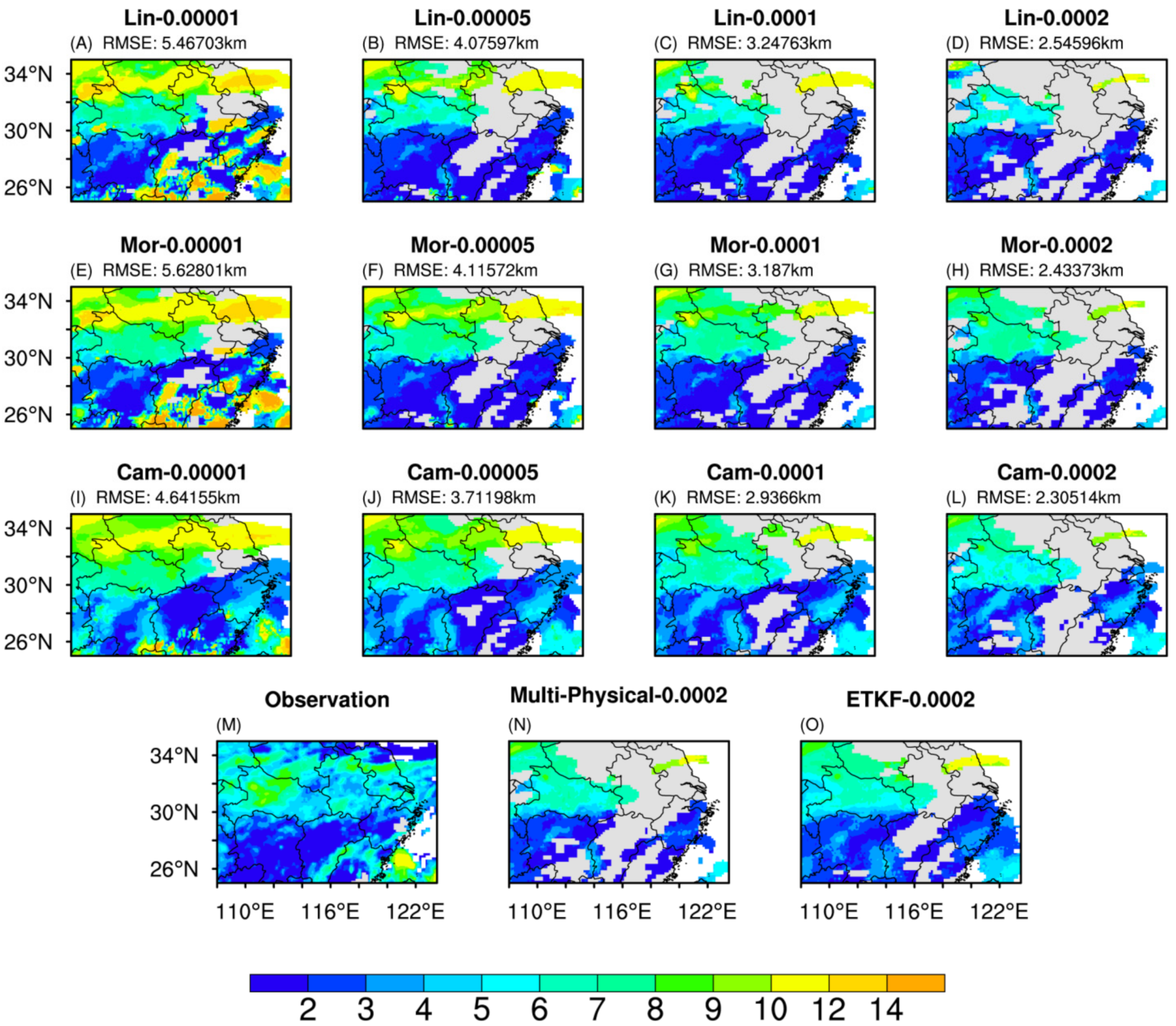
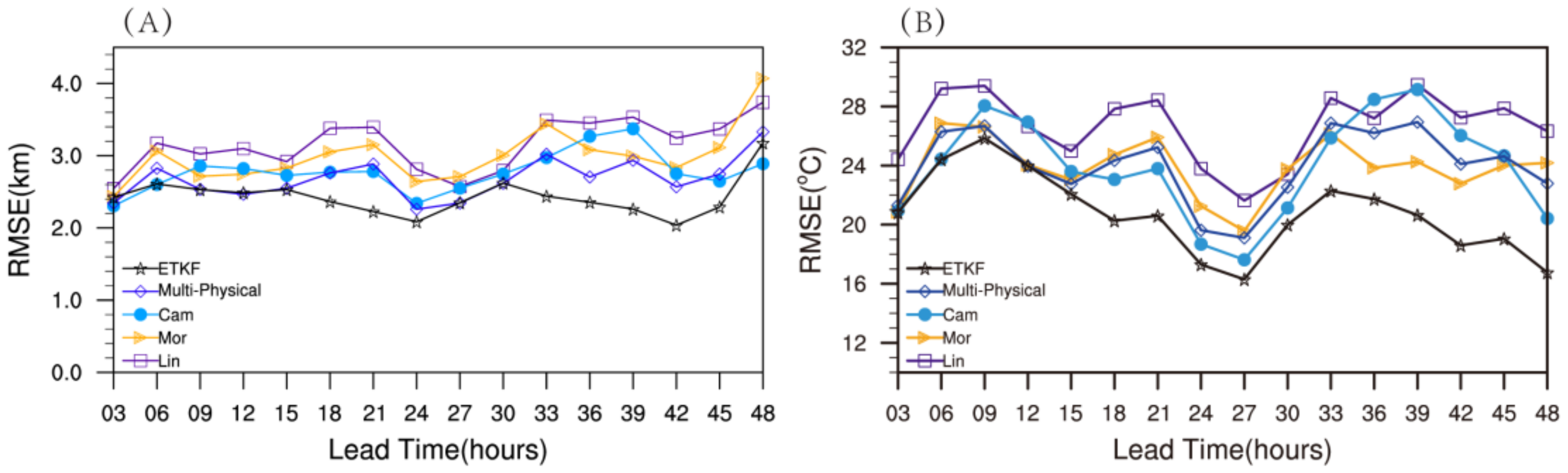
3.1. Cloud-Top Height and Temperature

Considering that different microphysical parameterization schemes may be suitable for different thresholds, several schemes are selected to test the sensitivity of four commonly used thresholds in eastern China. Figure 2 shows the evaluation results simulated by the Lin, Morrison 2-mom, and CAM5.1 microphysical parameterization schemes (hereinafter referred to as Lin, Mor, and Cam schemes) when the thresholds are taken as 10⁻⁵ kg∙kg⁻¹, 5 × 10⁻⁵ kg∙kg⁻¹, 10⁻⁴ kg∙kg⁻¹ and 2 × 10⁻⁴ kg∙kg⁻¹ [42]. In terms of the RMSE, it can be found that when the threshold is 10⁻⁵ kg∙kg⁻¹, the errors of the cloud-top height simulated by three different microphysical parameterization schemes are about 5 km, which is relatively large. When the threshold is 2 × 10⁻⁴ kg∙kg⁻¹, the RMSE is around 2.3–2.5 km, which is smaller than that of other thresholds. This result is consistent with Yang et al. [43], and in their study, the RMSE of the simulated cloud top height is around 2–3 km. Figure 2 shows the geographical distributions of cloud-top height simulated by the three schemes with different thresholds. Obviously, when the threshold is 10⁻⁵ kg∙kg⁻¹, the range of the simulated cloud system is wide close to the observation. However, the simulated cloud-top height errors are large in the north of 30° N, i.e., the cloud-top height of the observation is mainly around 5–8 km, while that of the simulation is about 9–12 km. When the threshold is 5 × 10⁻⁵ kg∙kg⁻¹, the range of the simulated cloud system is slightly smaller than that of the smaller threshold values, but the simulations in the north of 30° N are closer to the observation. When the threshold is 2 × 10⁻⁴ kg∙kg⁻¹, the prediction is more accurate than that of the threshold of 5 × 10⁻⁵ kg∙kg⁻¹. Therefore, it can be found that as the threshold value increases, the range of the simulated cloud system is smaller, and the forecast accuracy of the cloud-top height is improved. The same conclusions can be drawn from the geographical distribution map of cloud-top temperature (figure omitted). Zhao et al. [44] found that the GRAPES_Meso (the mesoscale version of the Global/Regional Assimilation and Prediction System) model has some deficiencies in simulating middle- and low-level clouds, such as underestimating cloud amount and cloud-top temperature and overestimating cloud-top height, which is similar to the results in this study based on the WRF.

Since the accurate prediction of cloud-top height and temperature is more important than that of the cloud system range during weather modification, the threshold value is set to 2 × 10⁻⁴ kg∙kg⁻¹ for the following ensemble prediction test. Figure 2 also shows the comparisons of the forecast results from two ensemble methods with the observation. The results indicate that the forecast accuracy of the cloud system range improved by the Multi-Physical is not obvious, but the ETKF has some improvements. In order to intuitively reflect the improvement of the Multi-Physical and ETKF, Figure 3 shows the RMSE sequence for 16 times of the research case. The results indicate that both methods reduce the errors to a certain extent, and the improvement of the ETKF is noticeable. From Figure 3A, it can be found that the RMSE values of the cloud-top height simulated by the Lin scheme are relatively large, while results from the CAM5.1 scheme are smaller, which can be more than 0.5 km smaller than those of Lin’s scheme at several moments. Compared with the optimal scheme (CAM5.1), the simulation results from the Multi-Physical are slightly improved, while the improvement of the ETKF is relatively greater, and the reduction in its RMSE can be up to about 1 km compared with the Lin scheme. As the forecast lead time increases, the RMSE of the cloud-top height simulated increases, and the improvement of the ETKF on the simulation is more remarkable. Figure 3B presents the RMSE sequence of cloud-top temperature simulated by three schemes and two ensemble methods. It can also be found that the CAM5.1 scheme has the smallest RMSE for most of the forecast lead time, up to 33 hours. The Multi-Physical is not effective in reducing the errors of cloud-top temperature, but the multi-physical ETKF with initial perturbation performs well, especially when the forecast lead time exceeds 33 hours. Therefore, it can be concluded that the multi-physical ETKF with initial perturbation has a remarkable effect on the correction of the cloud macro characteristic variables in this study.

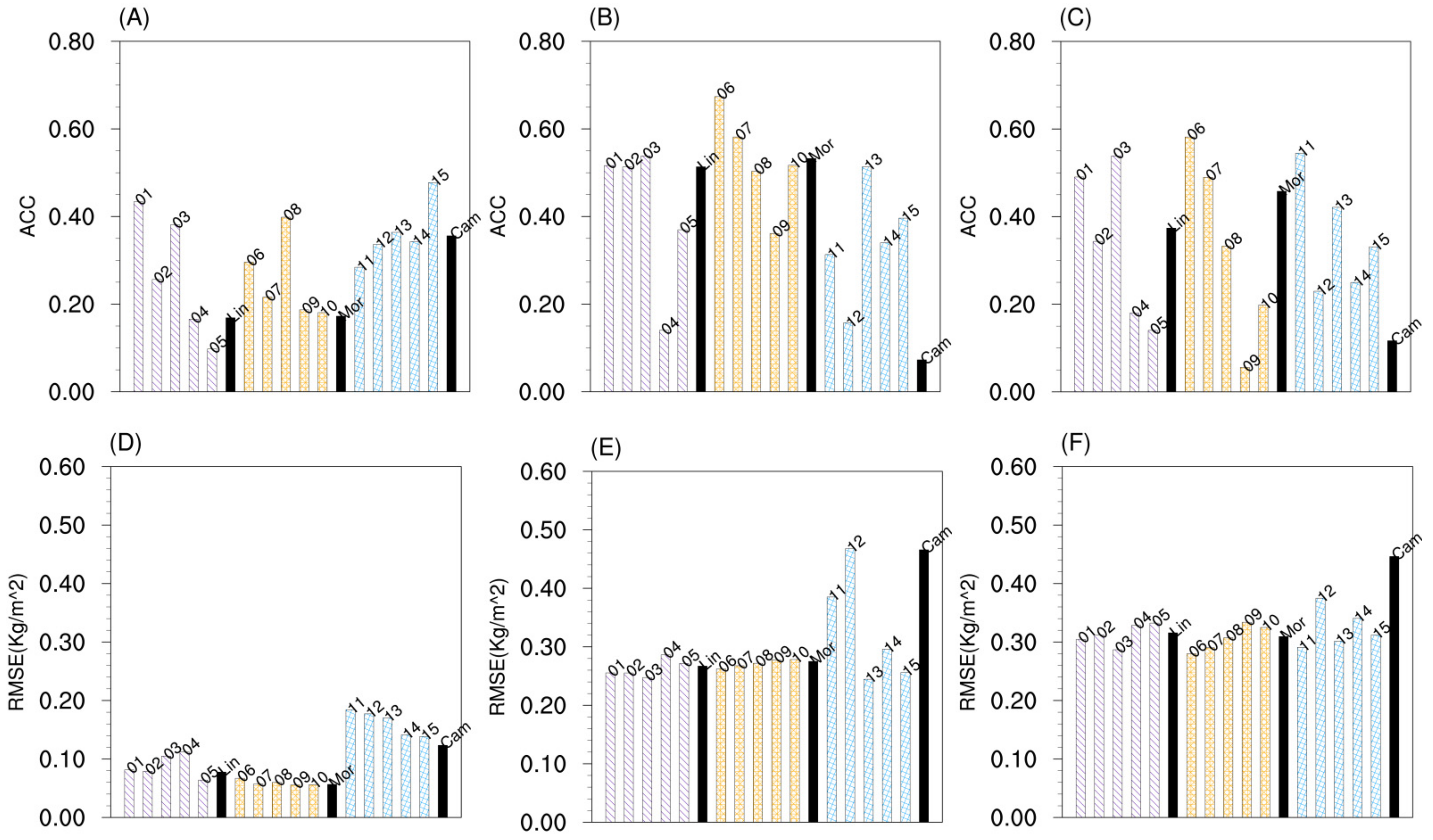
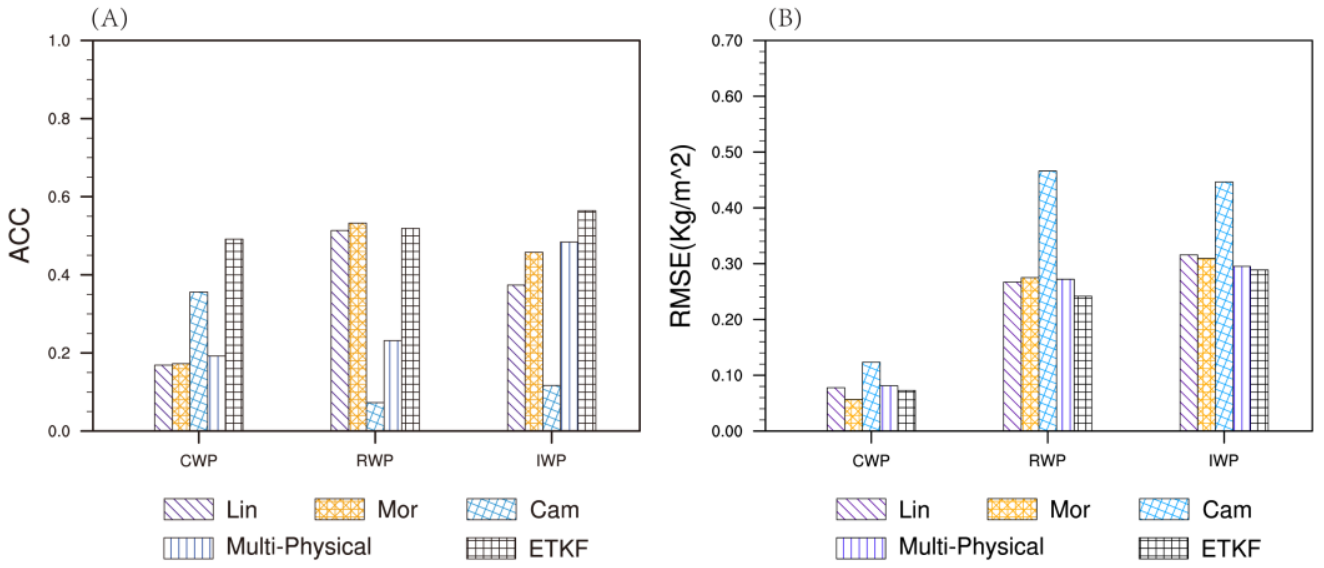
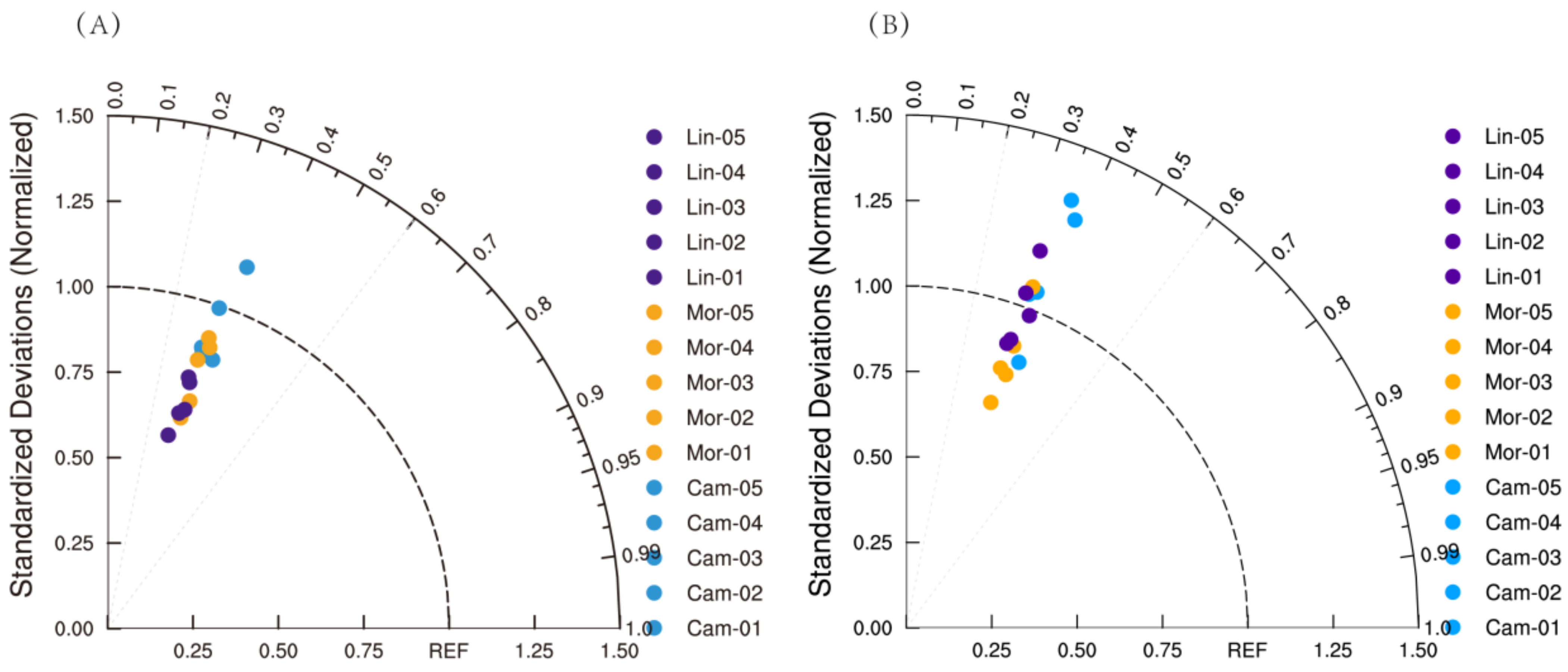
3.2. Cloud Hydrometeors

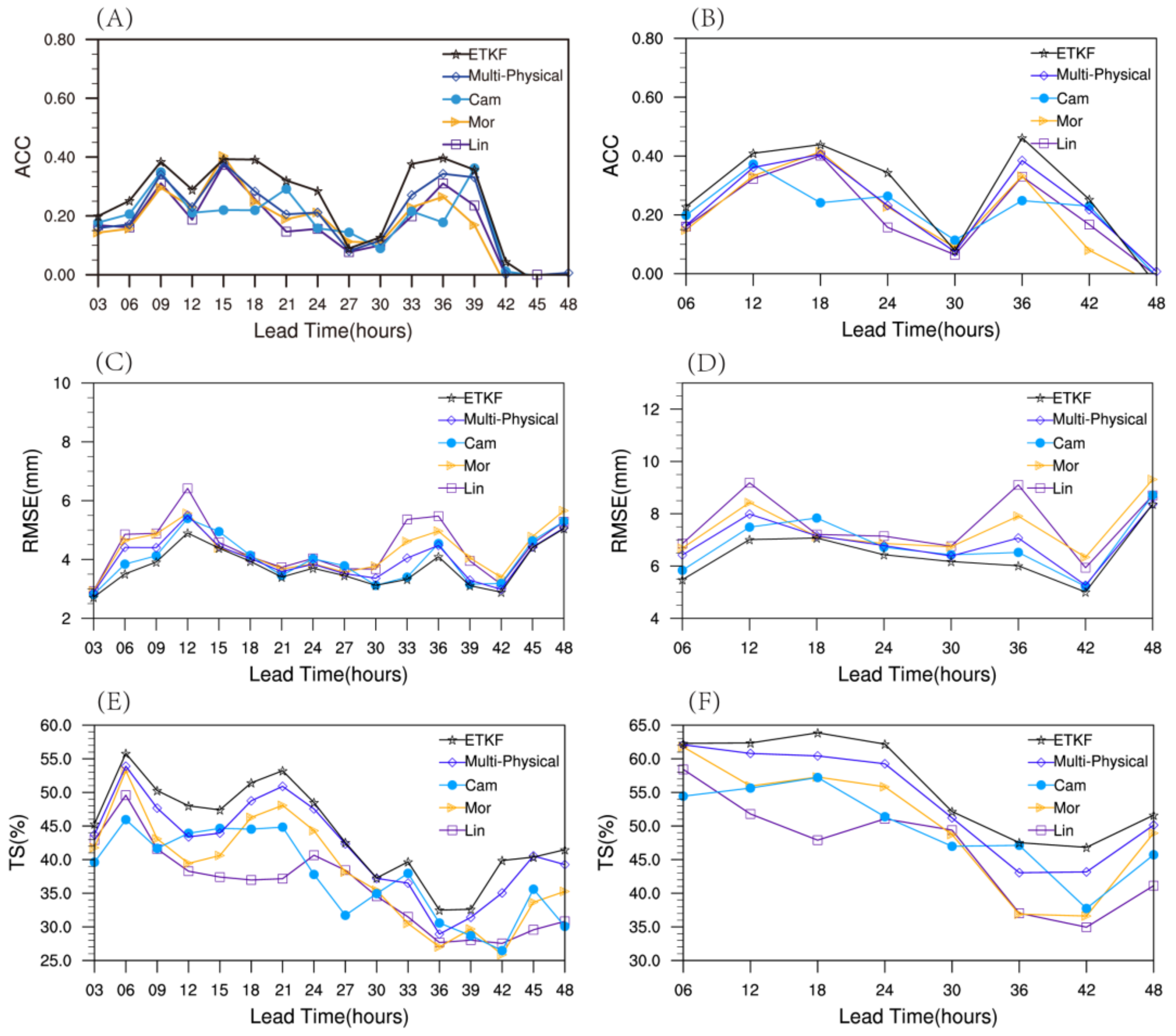
In addition to verifying that the ETKF can improve cloud-top height and temperature simulation, we conduct an ensemble forecast test for the hydrometeors in clouds. First, in this study, we analyze the simulations of all perturbed members of the ETKF, and Figure 4 displays the evaluation results of the cloud water, rainwater, and ice water obtained by the three schemes (Lin, Morrison 2-mom, and CAM5.1 schemes) without initial perturbation and the 15 perturbed members of the ETKF. The results suggest that under random initial perturbations, the evaluation results of each ensemble member of the ETKF are quite different, i.e., some ensemble members outperform the schemes without initial perturbation, while others do not. Moreover, the differences among ensemble members with different microphysical schemes are obvious.

Then, Figure 5A shows that the CAM5.1 scheme outperforms other schemes in simulating CWP, and the Morrison 2-mom scheme performs better in simulating RWP and IWP. However, Figure 5B indicates that the RMSE value of the CWP predicted by the CAM5.1 is worse than those of other schemes, and the RWP predicted by the Morrison 2-mom scheme is not optimal. In addition, the results of different evaluation methods are different, which also suggests that the three schemes have their own advantages and disadvantages. The comparison of the ETKF and Multi-Physical reveals that the Multi-Physical has limited improvements in the simulation of hydrometeors, while the improvements of the ETKF are noticeable. Specifically, The ACC values of the ETKF for the three hydrometeors are larger than the Multi-Physical, and the RMSE of the ETKF is 0.02–0.04 kg∙m⁻², lower than that of the Multi-Physical.

3.3. Precipitation

We explore the application of the ETKF in precipitation forecast based on the above methods. Figure 6 shows the Taylor diagrams of the 3-hour and 6-hour cumulative precipitation predicted by the 15 ensemble members of ETKF at 0600 UTC on August 12, 2014. The REF in the figure means the observations, the distance between a given forecast element and the origin point represents the standard deviation of the forecast element from the REF, the cosine of the azimuth of a given forecast field indicates its correlation with the REF, and the distance between the value of a given forecast element and the REF represents the root mean square error. It can be found that the standard deviations of the forecast results among the 15 ensemble members are quite different, indicating that different initial values and different microphysical schemes have a certain impact on the precipitation forecast. Comparing the evaluation results from the three schemes without initial perturbations (Lin, Morrison 2-mom, and CAM5.1 schemes), Multi-Physical and ETKF (Figure 7), we also find that the multi-physical ETKF with initial perturbations performs better than the Multi-Physical in the precipitation forecast. Overall, the RMSE, ACC, and threat score (TS) all show that the ETKF improves the precipitation simulation, and the improvement is larger than that of the Multi-Physical. For example, in terms of the 3-hour cumulative precipitation, the ETKF has up to 8% higher ACC, 5% higher TS, and 0.5 mm smaller RMSE than the Multi-Physical at some moments. The above analysis demonstrates that the different initial perturbations greatly impact the results of model precipitation forecast, and considering multiple initial perturbations in the Multi-Physical can improve the precipitation forecast of the heavy rainfall cases in this study.

4. Conclusions and Discussion

In this study, a large-scale precipitation case in summer is selected arbitrarily to investigate the simulations of cloud-top height and temperature, hydrometeors, and precipitation with different microphysical parameterization schemes in the WRF model. Subsequently, we perform a comparative experiment of simulations between the Multi-Physical and the ETKF. The conclusions are as follows.

When the threshold for calculating cloud-top height and temperature is 10⁻⁵ kg∙kg⁻¹, the simulated cloud system range is close to the observation, but the RMSE (5 km) of cloud-top height is large. When the threshold is 2 × 10⁻⁴ kg∙kg⁻¹, the simulated cloud system range is smaller than the observation, but the RMSE of cloud-top height is about 2.3–2.5 km. The ETKF can improve the forecast skills of cloud-top height and cloud-top temperature and outperforms the Multi-Physical in this study. Moreover, with the increase in forecast lead time, the improvement of the ETKF is more remarkable.

In terms of the hydrometeors forecast, the three parameterization schemes have their own advantages and disadvantages, and there is no obvious optimal scheme. The comparison between the ETKF and Multi-Physical suggests that the Multi-Physical offers limited improvements in the simulation of hydrometeors, while the improvements of the ETKF are noticeable. Specifically, The ACC values of the ETKF for the three hydrometeors are larger than that of the Multi-Physical, and the RMSE values of the ETKF are 0.02–0.04 kg∙m⁻², lower than those of the Multi-Physical. The ETKF combines the advantages of each parameterization scheme and makes up for the forecast instability of the schemes.

The ACC, RMSE, and TS suggest that the ETKF performs better than the Multi-Physical in the precipitation forecast. Specifically, the ETKF has up to 8% higher ACC, 5% higher TS, and 0.5 mm smaller RMSE than the Multi-Physical.

In this research, we obtain good results in the ETKF experiment of cloud simulation based on the WRF model. It is verified that the ETKF can effectively reduce the errors of model forecasts and provide more accurate guidance for weather modification operations. However, this experiment has a challenge in that it has a large number of calculations, and this method used in daily operations requires large computing resources. Due to the limitation of article length and calculation amount, the current work only explores the influence of different microphysical parameterization schemes on forecasts. In the following work, the influences of cumulus convection parameterization schemes and other schemes may be considered to further reduce forecast errors.

References

1. Guo, X.; Fu, D.; Li, X.; Hu, Z.; Lei, H.; Xiao, H.; Hong, Y. Advances in cloud physics and weather modification in China. Adv. Atmos. Sci. 2015, 32, 230–249. [Google Scholar] [CrossRef]
2. Flossmann, A.I.; Manton, M.; Abshaev, A.; Bruintjes, R.; Yao, Z. Review of advances in precipitation enhancement research. Bull. Am. Meteorol. Soc. 2019, 100, 1465–1480. [Google Scholar] [CrossRef]
3. Akdi, Y.; Ünlü, K.D. Periodicity in precipitation and temperature for monthly data of Turkey. Theor. Appl. Climatol. 2021, 143, 957–968. [Google Scholar] [CrossRef]
4. Wang, Z.M.; Letu, H.; Shang, H.Z.; Zhao, C.F.; Li, J.M.; Ma, R. A supercooled water cloud detection algorithm using Himawari-8 satellite measurements. J. Geophys. Res. Atmos. 2019, 124, 2724–2738. [Google Scholar] [CrossRef]
5. Xu, X.H.; Yin, J.F.; Zhang, X.T.; Xue, H.L.; Gu, H.D.; Fan, H.Y. Airborne measurements of cloud condensation nuclei (CCN) vertical structures over Southern China. Atmos. Res. 2022, 268, 106012. [Google Scholar] [CrossRef]
6. Qin, Y.S.; Cai, M.; Liu, S.X.; Cai, Z.X.; Hu, X.F.; Lue, F. A study on macro and micro physical structures of convective-stratiform mixed clouds associated with a cold front in autumn and their catalytic responses in North China. Acta Meteorol. Sin. 2017, 75, 835–849. [Google Scholar] [CrossRef]
7. Zheng, W.; Ma, H.; Zhang, M.; Xue, F.; Yu, K.; Yang, Y.; Ma, S.; Wang, C.; Pan, Y.; Shu, Z.; et al. Evaluation of the First Negative Ion-Based Cloud Seeding and Rain Enhancement Trial in China. Water 2021, 13, 2473. [Google Scholar] [CrossRef]
8. Rajeevan, M.; Kesarkar, A.; Thampi, S.B.; Rao, T.N.; Radhakrishna, B.; Rajasekhar, M. Sensitivity of WRF cloud microphysics to simulations of a severe thunderstorm event over Southeast India. Ann. Geophys. 2010, 28, 603–619. [Google Scholar] [CrossRef]
9. Dong, F.; Zhi, X.F.; Zhang, L.; Ye, C.Z. Diurnal variations of coastal boundary layer jets over the northern South China Sea and their impacts on diurnal cycle of rainfall over southern China during the early-summer rainy season. Mon. Weather Rev. 2021, 149, 3341–3363. [Google Scholar] [CrossRef]
10. Chung, K.-S.; Chiu, H.-J.; Liu, C.-Y.; Lin, M.-Y. Satellite Observation for Evaluating Cloud Properties of the Microphysical Schemes in Weather Research and Forecasting Simulation: A Case Study of the Mei-Yu Front Precipitation System. Remote Sens. 2020, 12, 3060. [Google Scholar] [CrossRef]
11. Yao, B.; Liu, C.; Yin, Y.; Zhang, P.; Min, M.; Han, W. Radiance-based evaluation of WRF cloud properties over East Asia: Direct comparison with FY-2E observations. J. Geophys. Res. Atmos. 2018, 123, 4613–4629. [Google Scholar] [CrossRef]
12. Cutraro, F.; Galligani, V.S.; Skabar, Y.G. Evaluation of synthetic satellite images computed from radiative transfer models over a region of South America using WRF and goes/16 observations. Q. J. R. Meteorol. Soc. 2021, 147, 2988–3003. [Google Scholar] [CrossRef]
13. Griffin, S.M.; Otkin, J.A. Evaluating the Impact of Planetary Boundary Layer, Land Surface Model, and Microphysics Parameterization Schemes on Simulated GOES-16 Water Vapor Brightness Temperatures. Atmosphere 2022, 13, 366. [Google Scholar] [CrossRef]
14. Griffin, S.M.; Otkin, J.A.; Nebuda, S.E.; Jensen, T.L.; Skinner, P.S.; Gilleland, E.; Supinie, T.A.; Xue, M. Evaluating the impact of planetary boundary layer, land surface model, and microphysics parameterization schemes on cold cloud objects in simulated GOES-16 brightness temperatures. J. Geophys. Res. Atmos. 2021, 126, e2021JD034709. [Google Scholar] [CrossRef]
15. Zhang, D.L. Roles of Various Diabatic Physical Processes in Mesoscale Models. Chin. J. Atmos. Sci. 1998, 22, 548–561. [Google Scholar] [CrossRef]
16. Dawn, S.; Satyanarayana, A.N.V. Sensitivity studies of cloud microphysical schemes of WRF-ARW model in the simulation of trailing stratiform squall lines over the Gangetic West Bengal region. J. Atmos. Sol.-Terr. Phys. 2020, 209, 396–420. [Google Scholar] [CrossRef]
17. Venkata, R.G.; Venkata, R.K.; Sridhar, V. Sensitivity of Microphysical Schemes on the Simulation of Post-Monsoon Tropical Cyclones over the North Indian Ocean. Atmosphere 2020, 11, 1297–1313. [Google Scholar] [CrossRef]
18. Cintineo, R.; Otkin, J.A.; Xue, M.; Kong, F. Evaluating the performance of planetary boundary layer and cloud microphysical parameterization schemes in convection-permitting ensemble forecasts using synthetic goes-13 satellite observations. Mon. Weather Rev. 2014, 142, 163–182. [Google Scholar] [CrossRef]
19. Pu, Z.X.; Lin, C.; Dong, X.Q.; Krueger, S.K. Sensitivity of Numerical Simulations of a Mesoscale Convective System to Ice Hydrometeors in Bulk Microphysical Parameterization. Pure Appl. Geophys. 2019, 176, 2097–2120. [Google Scholar] [CrossRef]
20. Huang, Y.J.; Wang, Y.P.; Xue, L.L.; Wei, X.L.; Zhang, L.N.; Li, H.Y. Comparison of three microphysics parameterization schemes in the WRF model for an extreme rainfall event in the coastal metropolitan City of Guangzhou, China. Atmos. Res. 2020, 240, 104939. [Google Scholar] [CrossRef]
21. Ma, X.L.; Xue, J.S.; Lu, W.S. Preliminary study on ensemble transform Kalman filter-based initial perturbation scheme in GRAPES global ensemble prediction. Acta Meteorol. Sin. 2008, 66, 526–536. [Google Scholar] [CrossRef]
22. Zhang, H.B.; Chen, J.; Zhi, X.F.; Wang, Y.N. A Comparison of ETKF and Downscaling in a Regional Ensemble Prediction System. Atmosphere 2015, 6, 341–360. [Google Scholar] [CrossRef]
23. Chen, C.; Li, C.Y.; Tan, Y.; Zeng, Y.; Zhou, Z. Study of the drift of ensemble forecast effects caused by stochastic forcing. Acta Meteorol. Sin. 2013, 3, 505–516. [Google Scholar] [CrossRef]
24. Wang, J.Z.; Chen, J.; Zhang, H.B.; Tian, H.; Shi, Y.N. Initial perturbations based on ensemble transfrom kalman filter with rescaling method for ensemble forecast. Weather Forecast. 2021, 36, 823–842. [Google Scholar] [CrossRef]
25. Zhou, X.Q.; Zhu, Y.J.; Hou, D.C.; Daryl, K. A Comparison of Perturbations from an Ensemble Transform and an Ensemble Kalman Filter for the NCEP Global Ensemble Forecast System. Weather Forecast. 2016, 31, 2057–2074. [Google Scholar] [CrossRef]
26. Zhang, J.; Feng, J.; Li, H.; Zhu, Y.J.; Zhi, X.F.; Zhang, F. Unified ensemble mean forecasting of tropical cyclones based on the feature-oriented mean method. Weather Forecast. 2021, 36, 1945–1959. [Google Scholar] [CrossRef]
27. Feng, J.; Zhang, J.; Toth, Z.; Peña, M.; Ravela, S. A New Measure of Ensemble Central Tendency. Weather. Forecast. 2020, 35, 879–889. [Google Scholar] [CrossRef]
28. Bishop, C.; Etherton, B.J.; Majumdar, S.J. Adaptive Sampling with the Ensemble Transform Kalman Filter. Part I: Theoretical Aspects. Mon. Weather Rev. 2001, 129, 420–436. [Google Scholar] [CrossRef]
29. Peffers, L.T. Hybrid Variational Ensemble Data Assimilation with Initial Condition and Model Physics Uncertainty. Ph.D. Thesis, The Florida State University, Tallahassee, FL, USA, 2011. [Google Scholar]
30. Zhang, H.B.; Chen, J.; Zhi, X.F.; Long, K.J.; Wang, Y.N. Design and comparison of perturbation schemes for GRAPES—Meso based ensemble forecast. Trans. Atmos. Sci. 2014, 37, 276–284. [Google Scholar] [CrossRef]
31. Huang, H.Y.; Qi, L.L.; Liu, J.W.; Huang, J.P.; Li, S.Y. Preliminary application of a multi-physical ensemble transform Kalman filter in precipitation ensemble prediction. Chin. J. Atmos. Sci. 2016, 40, 657–668. [Google Scholar] [CrossRef]
32. National Centers for Environmental Prediction-Final Operational Global Analysis Data. Available online: http://dss.ucar.edu/datasets/ds083.2 (accessed on 15 March 2021).
33. Lin, Y.L.; Farley, R.D.; Orville, H.D. Bulk parameterization of the snow field in a cloud model. J. Appl. Meteorol. 1983, 22, 1065–1092. [Google Scholar] [CrossRef]
34. Morrison, H.; Thompson, G.; Tatarskii, V. Impact of Cloud Microphysics on the Development of Trailing Stratiform Precipitation in a Simulated Squall Line: Comparison of One- and Two-Moment Schemes. Mon. Weather Rev. 2009, 137, 991–1007. [Google Scholar] [CrossRef]
35. Eaton, B. User’s Guide to the Community Atmosphere Model CAM-5.1. NCAR. Available online: http://www.cesm.ucar.edu/models/cesm1.0/cam (accessed on 15 March 2021).
36. Beljaars, A.C.M. The parametrization of surface fluxes in large-scale models under free convection. Q. J. R. Meteorol. Soc. 1995, 121, 55–270. [Google Scholar] [CrossRef]
37. Mlawer, E.J.; Taubman, S.J.; Brown, P.D.; Lacono, M.J.; Clough, S.A. Radiative transfer for inhomogeneous atmospheres: RRTM, a validated correlated-k model for the longwave. J. Geophys. Res. Atmos. 1997, 14, 16663–16682. [Google Scholar] [CrossRef]
38. Dudhia, J. Numerical study of convection observed during the winter monsoon experiment using a mesoscale two-dimensional model. J. Atmos. Sci. 1989, 46, 3077–3107. [Google Scholar] [CrossRef]
39. Chen, F.; Dudhia, J. Coupling an Advanced Land Surface Hydrology Model with the Penn State NCAR MM5 Modeling System. Part I: Model Implementation and Sensitivity. Mon. Weather Rev. 2001, 4, 569–585. [Google Scholar] [CrossRef]
40. Hong, S.Y.; Noh, Y.; Dudhia, J. A New Vertical Diffusion Package with an Explicit Treatment of Entrainment Processes. Mon. Wea. Rev. 2006, 9, 2318–2341. [Google Scholar] [CrossRef]
41. Climate Prediction Center Morphing Technique Data. Available online: http://data.cma.cn/data/detail/dataCode (accessed on 15 March 2021).
42. Wu, W. Comparison to the Sensitivity of GRAPES and WRF Model Cloud Microphysical Parameterization Schemes Using CloudSat and MODIS Satellite Data. Master’s Thesis, Lanzhou University, Lanzhou, China, 2011. [Google Scholar]
43. Yang, Y.; Sun, W.; Chi, Y.; Yan, X.; Fan, H.; Yang, X.; Ma, Z.; Wang, Q.; Zhao, C. Machine learning-based retrieval of day and night cloud macrophysical parameters over East Asia using Himawari-8 data. Remote Sens. Environ. 2022, 273, 112971. [Google Scholar] [CrossRef]
44. Zhao, C.Y.; Xu, G.Q.; Huang, S.Y. Preliminary Experimental Study on Improving Cloud Computing Process with Satellite Data. Meteorol. Mon. 2020, 46, 1585–1595. [Google Scholar] [CrossRef]
Figure 1. The simulation domain of the WRF.
Atmosphere 13 01359 g001
Figure 2. Geographical distribution comparison of the cloud-top height (km) between the simulations for four thresholds at 0600 UTC on 12 August 2014 by the (AD) Lin, (EH) Morrison 2-mom, (IL) CAM5.1 microphysical parameterization schemes and (N) Multi-Physical, (O) ETKF, (M) the satellite observation data and their root mean square errors (RMSE).
Atmosphere 13 01359 g002
Figure 3. RMSE sequence of the (A) cloud-top height and (B) temperature simulated by three schemes and two ensemble methods.
Atmosphere 13 01359 g003
Figure 4. The ACC and RMSE (kg∙m−2) of the (A,D) cloud water path, (B,E) rainwater path, and (C,F) ice water path simulated by the 3 schemes (black filled bars) and the 15 perturbed members of the multi-physical ETKF with Lin, Morrison 2-mom, CAM5.1 microphysical parameterization schemes on 12 August 2014. The purple-filled bars (01–05) denote the results of the 5 perturbed members adopting the Lin scheme, the yellow-filled bars (06–10) indicate the results of the Morrison 2-mom scheme, the blue-filled bars (11–15) represent the results of the CAM5.1 scheme.
Atmosphere 13 01359 g004
Figure 5. The (A) anomaly correlation coefficients (ACC) and (B) RMSE (kg∙m−2) of hydrometeors simulated by the three schemes and two ensemble methods.
Atmosphere 13 01359 g005
Figure 6. Taylor diagrams of the 3-hour (A) and 6-hour (B) accumulated precipitation simulated by the 15 perturbation members of ETKF at 0600 UTC on 12 August 2014. Purple represents results from Lin’s scheme, yellow indicates results from the Morrison 2-mom scheme, and blue denotes results from the CAM5.1 scheme.
Atmosphere 13 01359 g006
Figure 7. The ACC, RMSE, and threat scores of the (A,C,E) 3-hour and (B,D,F) 6-hour accumulated precipitation simulated by three schemes and two ensemble methods for different forecast lead times.
Atmosphere 13 01359 g007