Article

The Consistent Variations of Precipitable Water and Surface Water Vapor Pressure at Interannual and Long-Term Scales: An Examination Using Reanalysis

Key Laboratory of Meteorological Disaster, Ministry of Education, Joint International Research Laboratory of Climate and Environment Change, Collaborative Innovation Center on Forecast and Evaluation of Meteorological Disasters, Nanjing University of Information Science and Technology, Nanjing 221000, China
*
Author to whom correspondence should be addressed.
Atmosphere 2022, 13(9), 1350; https://doi.org/10.3390/atmos13091350
Submission received: 2 July 2022 / Revised: 22 August 2022 / Accepted: 22 August 2022 / Published: 24 August 2022

Abstract

:
Water vapor (WV) is a vital basis of water and energy cycles and varies with space and time. When researching the variations of moisture in the atmosphere, it is intuitive to think about the total WV of the atmosphere column, precipitable water (PW). It is an element that needs high-altitude observations. A surface quantity, surface WV pressure (SVP), has a close relationship to PW because of the internal physical linkage between them. The stability of their linkage at climatic scales is verified using monthly mean data from 1979 to 2021, while studies before mainly focused on daily and annual cycles in local areas. The consistency of their variations is checked with three reanalysis datasets from three angles, the interannual variations, the long-term trends, and the empirical orthogonal function (EOF) modes. Results show that the interannual correlation of SVP and PW can reach a level that is quite high and are significant in most areas, and the weak correlation mainly exists over low-latitude oceans. The long-term trends, as well as the first EOF modes of these two quantities, also show that their variations are consistent, with spatial correlation coefficients between the long-term trends of two variables that are generally over 0.6, but specific differences appearing in some regions including the Tropical Indian Ocean and Middle Africa. With the correspondence of PW and SVP, the variations of total column WV can be indicated by surface elements. The correspondence is also meaningful for the analysis of the co-variation in total column vapor and temperature. For example, we could research the relations between SVP and air temperature, and they can reflect the co-variance of total column vapor and near-surface air temperature, which can avoid analyzing the relation between column-integrated moisture content and surface air temperature directly.

1. Introduction

As a component in the global water and energy cycles, atmospheric WV is also an important part of climate variability and change [1,2,3]. WV is the material basis of precipitation, and the latent heat released by precipitation is a part of the energy cycle and can drive atmospheric circulation anomalies [4,5]. The circulation may, in turn, transport WV, and change the spatiotemporal distribution of the WV [6]. As the most abundant greenhouse gas in the atmosphere, WV also affects the atmospheric radiation processes [7].
PW, a conventional quantity of humidity, is the column-integrated WV amount in the atmosphere [8]. In a regional air column, the WV evaporated from the surface, along with the WV converged from the surroundings, is used to increase the PW. When the air saturates, at least at certain levels, precipitation may be produced. In the past, acquirement of PW data nearly always relied on radiosonde observations [9,10]. Because of the high costs of radiosonde and the sparsity of observation stations, studies about empirical equations between PW and surface elements appeared. A surface quantity, SVP, has been stressed that has a close statistical linkage to PW [11,12,13,14]. This linkage can also be explained from a physical aspect. In essence, SVP can be regarded as the force exerted by the total moisture in the air column [15], in analogy with the surface pressure to the total mass of the air column. From another point of view, WV content is maximal at the near-surface level and decreases with altitude because of the existence of gravity. Hence, the SVP can well represent the column WV content [16,17]. Due to the lack of upper-air detections, the empirical relations between PW and SVP were utilized to estimate the PW with surface observations in local areas, especially during the early stage of this methodology when there were just a few sounding observations [18,19,20,21]. Some advanced methods can currently be used to obtain PW data, such as ground-based radar observations, satellite retrievals [22,23], global position system (GPS) observations [24,25], model outputs, and the reanalysis [26,27]. Because of the high spatial and temporal resolution of remote sensing products, which could be 1 h and 30 km, they can help to fill the gaps between radiosonde locations and launch times. However, the retrieval effects except for microwave-based products are often not very useful in cloudy areas [22,23]. The ground-based GPS data have a higher temporal resolution, which is about 5 min [25], but the network is not so dense, and the duration is relatively short. Except for a few elements such as precipitation, the reanalysis datasets universally have decent accuracy in broad areas, with the support of the accumulations of vast amounts of historical observations, advanced modeling, and data assimilation systems. They have been applied in studies on the hydrological fields and their effects have been verified [8].
Because of the appearance of these measuring methods, perhaps the demands of calculating PW with surface elements are not as imperious as earlier. However, analyzing the relationship between them is still meaningful. It is easy to understand that over areas with few instructions, such as oceans, the SVP can be calculated with PW retrieved by satellite remote sensing.
Numerous studies have proven the quasi-linear relation between SVP and PW from the statistical aspect, and there are empirical equations in local areas [19,21,28,29]. Due to the appearance of progressive observation methods such as satellite remote sensing, the PW data can be used to estimate the values of SVP in reverse in the areas where it is hard to establish observation stations [20]. Previous studies are mainly concentrated on daily and annual cycles in local areas when analyzing the relationship between PW and SVP. Their relationship at interannual scales was researched in a few studies, but most of them still focused on the linkage in local areas. In daily or seasonal variations, the radiation processes vary dramatically, so following the temperature, PW, and SVP both have obvious variations, and it may be easy to vary consistently for them. When analyzing the interannual or long-term variations, the amplitudes may be much smaller. The questions researched here are whether the consistency is reliable at climatical scales, and where the consistency is not good. Hence, the consistency of interannual and long-term variations of monthly mean PW and SVP are examined globally.
Under global warming, atmospheric moisture is often linked to tropospheric temperature or surface air temperature through Clausius–Clapeyron Equation [30,31,32,33,34]. Many researchers studied the interannual and long-term variations of WV as well as its relationship with temperature, using PW or SVP [3,35,36,37,38]. Globally, the WV follows the temperature closely in line with the Clausius–Clapeyron Equation. However, it is more exhausted when researching the variation in local areas [39]. The PW in some areas has decreasing trends, such as in Australia from 1957–2016 [37]. As for the interannual variation in WV, Hao and Lu [39] studied the response of SVP to surface air temperature and found that the response of SVP to temperature is in close line with the Clausius–Clapeyron Equation at high latitudes. Shi et al. [40] studied the relationship between upper troposphere humidity and PW. Some studies also researched the linkage between PW and surface air temperature and re-established the PW during periods that lack high-altitude observations [41,42]. Wang et al. [8] found that there is a close linkage between the first EOF mode of PW and the Niño-3.4 index. As introduced before, the surface quantity which can directly reflect the PW is SVP. Because of the physical relation between SVP and surface air temperature, there is also a tight linkage between PW and the latter.
The long-term and interannual variations of total WV in the atmosphere can be reflected by SVP if the variations of the two quantities are consistent. When studying the response of WV to temperature, it is more suitable to use SVP than PW because the quantities that are all at the surface level can be used. It can avoid the problems brought by linking the column-integrated moisture with surface-level temperature or integrating the intensive quantities. With the linkage between PW and SVP, the response of SVP to the temperature studied in [39] can be extended to that of PW to a certain degree, while the response of SVP to surface temperature is studied in another part of our work.
Consulting the internal physical relation between PW and SVP, their linkage may be stable when the atmosphere is in hydrostatic equilibrium because the vertical movements can break the direct relationship between mass and pressure of the fluid. In the areas where the convection is active, the monthly averages of vertical motions are strong and precipitation amounts are large. The climatic value of PW and SVP are both larger than in other areas, but the linear correlation between monthly mean PW and SVP are probably weaker. Hence, in some areas, it could be hard to establish an efficient empirical equation between PW and SVP, and these areas could be found in the study.
The linkage between PW and SVP is analyzed from three angles concurrently. The interannual correlation and long-term trends of them are examined globally. Different from the daily or annual cycles, the interannual and long-term variations of these two physical variables may be much smaller. Hence, whether the linkage between them is still stable and where their linkage is not so good when analyzing their interannual and long-term variations are the questions that we tried to answer. To further verify the consistency of their variations, the first EOF modes of PW and SVP are shown and compared as well. To further verify the credibility of the results, three reanalysis datasets from different institutions are used. Due achieve this, we may mainly focus on the common points among the three datasets in the analysis.
The datasets together with the methods adopted are presented in Section 2. The consistency of interannual variations and long-term trends of PW and SVP are shown in Section 3.1 and Section 3.2. The EOF leading modes and time series are compared in Section 3.3. Section 4 shows the summary and discussion.

2. Data and Method

2.1. Data

Except for a few elements such as precipitation, the reanalysis datasets universally own decent accuracy in broad areas, with the support of the accumulations of vast amounts of historical observations, advanced modeling, and data assimilation systems. They have been applied in studies on the hydrological fields and their effects have been verified [8]. With the aim of the global scale study and ensuring the credibility of the results, three reanalysis datasets from different institutions are used, the European Centre for Medium-Range Weather Forecasts (ECMWF) Reanalysis v5 (ERA5), Japanese 55-year Reanalysis (JRA55), and the National Centers for Environmental Prediction and the Department of Energy (NCEP-DOE) Reanalysis-2 (NCEP2).
The ERA5 [43], provided by the ECMWF, is the fifth-generation ECMWF atmospheric reanalysis of the global climate covering the period from January 1950 to the present. ERA5 is produced by the Copernicus Climate Change Service (C3S) at ECMWF. The data cover the Earth on a 30 km grid and resolve the atmosphere using 137 levels from the surface up to a height of 80 km. The NCEP2 project performs data assimilation using past data from 1979 through the previous year [44].
Spanning from 1958 to present, JRA-55 is the longest third-generation reanalysis that uses the full observing system. Compared to the previous generation Japanese Meteorological Agency (JMA) reanalysis (JRA-25), JRA-55 uses a more advanced data assimilation scheme, increased model resolution, a new variational bias correction for satellite data, and several additional observational data sources [45]. Horizontal resolutions of the three datasets are all 2.5° × 2.5° in latitude and longitude.
The quantities used include the monthly mean PW, the 2 m temperature, and the 2 m dewpoint temperature from 1979 to 2021, which are directly downloaded from the servers. The SVP and saturated SVP are calculated with the modified Tetens formula [46], then the relative humidity can be obtained. As for the quantities at pressure levels, the moisture-related quantity directly given by ERA5 and JRA55 is specific humidity and that given by NCEP2 is relative humidity. Utilizing one of them with temperature which can be downloaded from the server, the other one can be figured out. The specific processes are illustrated below. With the temperature data, the saturated WV pressure can be calculated firstly as mentioned before. Then, with the relative humidity, the WV pressure can be archived. Finally, the specific humidity q can be obtained with the approximate empirical equation q = ε(e/p), where e is WV pressure and p is the pressure. The ratio of dry and wet gas constant ε is taken as 0.622 here. To analyze the profiles, the vertical velocity at pressure levels is also used and directly downloaded. There are 12 isobaric levels from 1000 hPa to 100 hPa in all three datasets used in the paper. The specific levels can be seen in the plots that show vertical profiles. Because the surface levels of the chosen land areas are general over 1000 hPa, the lowest level shown in land areas is 925 hPa. To intuitively show the variables downloaded and calculated, they are listed in Table 1.

2.2. Method

2.2.1. Mann–Kendall Test and Sen’s Slope Estimator

There are some ways to estimate the trends of hydrological and meteorological elements, including parametric and non-parametric methods [47]. Analysis of long-term trends includes the confirmation of increasing or decreasing slopes and significance testing [48]. Mann–Kendall test was formulated by Mann [49] as a non-parametric test for trend detection, and the test statistic distribution was given by Kendall [50] for testing non-linear trends and turning points. It is an excellent non-parametric method and is preferred by many researchers [51]. It is used for trend analysis, as it eliminates the effect of serial dependence on auto-correlated data which modifies the variance of datasets [52]. The MK test is used to test the significance of long-term trends of PW and SVP.
Sen’s slope estimation, also a non-parametric method, gives the magnitude of the trend [53]. Another advantage of Sen’s slope is that it is not affected by outliers and single data errors in the dataset [54].
The slopes of the long-term trends are calculated with the Theil–Sen slope estimator, and it is also a non-parametric method [53]. In this model, the slope values reflect the increasing and decreasing magnitudes of variables. The long-term trends of PW and SVP at each grid are calculated with this method to examine their consistency.

2.2.2. Empirical Orthogonal Function (EOF) Analysis

In climate research, EOF analysis is often used to study possible spatial modes of variability and how they change with time. In statistics, EOF analysis is known as Principal Component Analysis (PCA) [55]. As such, EOF analysis is sometimes classified as a multivariate statistical technique. A field is partitioned into mathematically orthogonal modes which can be called EOF spatial modes, or patterns. Typically, the EOFs are found by computing the eigenvalues and eigenvectors of a spatially weighted anomaly co-variance matrix of a field. The derived eigenvectors just vary with spatial modes. Each of the eigenvectors is an EOF pattern. The derived eigenvalues provide a measure of the percent variance explained by each mode. The time series (principal components) of each spatial pattern are determined by projecting the derived eigenvectors onto the spatially weighted anomalies. This will result in the amplitude of each mode over the period of record. Each pair of spatial patterns and time series can represent the spatial-temporal varying features of the variable.
By construction, the EOF patterns and the principal components are independent. Two factors inhibit physical interpretation of EOFs. One is the orthogonality constraint and the other is that the derived patterns may be domain-dependent. Physical systems are not necessarily orthogonal and if the patterns depend on the region used, they may not exist if the domain changes. Still, even with these shortcomings, classical EOF analysis has proved to be useful.
To make sure the EOF modes of PW and SVP are distinguished from the noise signal, the Monte Carlo technique [56] is used to test the significance of the first three modes.

2.2.3. The Theoretical Linkage between PW and SVP

PW is the total WV amount in the atmosphere column and can be expressed as the integration of the WV from the surface to the tropopause. Under the condition of hydrostatic equilibrium, the equation can be transferred to the isobaric coordinate form. The σ-coordinate σ ≡ p/ps is employed and specific humidity is expressed with WV pressure as q = ε(e/p). As shown by Lu [17], the PW can be written as
W = ε g 0 1 ed ln σ
In equations, the PW is denoted as W. The vapor pressure e normally reaches its maximum at surface level, then decreases with the altitude [57]. Vapor pressure can be seen as a function of σ approximately and expressed as e = Eσm. In the formula, SVP is denoted as E, and m is a constant in a specific area. Then, the relationship between PW and SVP can be expressed as W = k∙E, and k is expressed as k = ε/(gm) in the formula, where g is gravitational acceleration and m is the constant described before. As a result, W has a close linkage with surface vapor pressure E.
From another point of view, SVP is produced by the gravity of total WV in the air column and their linkage is the same as the relationship between surface pressure and the total quality of the column air mass. Hence, if the atmosphere is in hydrostatic equilibrium, there will be a linear linkage between PW and SVP.

3. Results

3.1. The Consistency of Interannual Variations

Figure 1 shows the maps of interannual correlation coefficients of monthly mean PW and SVP calculated with the ERA5 dataset. (The long-term trends are removed before calculating the correlation coefficient. Results obtained with JRA55 and NCEP2 are shown in Figures S1 and S2 in the Supplementary Materials). Three datasets all show that the coefficients in most areas are positive and can pass the 0.05 significance level, except in July. Just a few areas cannot pass the significance test and they are almost all in low-latitude regions. As illustrated before, the stratification of the tropical atmosphere is less stable, and the more frequent convection there probably breaks the linear relationship between PW and SVP. The linear correlation is especially strong in some areas, such as the Antarctic, Australia, Eurasian Continents, and the Southern Ocean. The distributions of strong correlation areas (SCAs) are similar among the three datasets.
Comparing the results calculated with different datasets, the weak correlation areas (WCAs) accordant among three datasets in all four months include the Maritime Continent, coasts of the Tropical Atlantic, the north coast of the Indian Ocean, and the east coast of the Southeast Pacific. There also exist differences among different datasets. Overall, insignificant correlation areas of NCEP2 and JRA55 are larger than those of ERA5. In JRA55, there are more WCAs in the Arctic in July. In NCEP2, there are more WCAs in the North Pacific in July and east Equatorial Pacific in July and October.
As for temporal variations, insignificant correlation areas in July are much larger than those in other months. The correlation coefficients at high latitudes in January, April, and October are large and can reach the 0.05 significance level. Differently, there exist some WCAs at mid-to-high latitudes in the Northern Hemisphere in July. It is plausible that this pattern is also relevant to stronger convection in these areas in Boreal Summer. Synthetically, the distribution of weak correlation areas, to some degree, is similar to the position and shape of the Inter Tropical Convergence Zone (ITCZ), with relatively larger areas in the West Pacific and the Indian Ocean and integrally more northward locations. The narrow belt distribution over other tropical oceans of the weak correlations is also slightly similar to the features of ITCZ.
When analyzing the monthly mean values, the areas with stronger convection could have stronger upward motion and a larger amount of precipitation. As mentioned, the linear relation between PW and SVP will be strong in hydrostatic equilibrium. In areas with strong and frequent convection, the interannual variation in vertical motion may also be stronger compared to the stable areas. The fluctuation of vertical movements will break the physical relation between quality and pressure. Hence, the weaker correlation areas in Figure 1 over oceans are probably associated with strong convection, and this is simply checked in the next section.
Results of the three datasets uniformly show that PW and SVP are strongly correlated in most extratropical areas and prove their strong linear relationship. The spatial patterns of correlation coefficients in extratropical areas are also concurrent among the three datasets, except for the weaker correlation in the Arctic in July obtained with JRA55.
The curves of normalized PW and SVP in red and blue squares in Figure 1, Figures S1 and S2 are also examined, but not shown in the main text (results are shown in Figures S3–S6 in the Supplementary Material). The variations of PW and SVP in SCAs can be quite consistent both on land and over the ocean. As for those in WCAs, on land, it seems that the variations of two variables are relatively more consistent before 1997, but this phenomenon cannot be seen over the oceans. Whether it is due to the data quality or other signals of the atmosphere variability needs further analysis.
To preliminarily analyze the reasons for the weak correlation in some areas, the vertical profiles of specific humidity and vertical velocity are exhibited. On land, the weak correlation area is in North Africa in places such as the Sahara. The vertical lapse rates are larger and more like exponential curves in SCAs (Figure 2). Due to the extreme drought in the WCAs, the WV differences between middle and low levels are relatively small compared with the SCAs. Hence, the influence of humidity at middle levels is relatively larger. Additionally, the standard deviation at middle levels is larger than that at low levels in WCAs, while the condition is reversed in the SCAs. The large ratio of fluctuations at middle levels to those at low levels can break the linear relation between PW and SVP because a large part of PW variation is at middle levels.
Over the oceans, the specific humidity in the WCAs is more than that in the SCAs from the lower to upper troposphere (Figure 3). However, the lapse rate seems larger in the SCAs below 700 hPa. The standard deviation at middle levels is larger than that at low levels both in strong and correlation areas. The fluctuations at low levels in the WCAs are nearly zero, and it is hard for SVP, with almost no variation, to reflect the variation in PW. The small fluctuations there may be caused by the frequent convection, and the surface air is nearly saturated all the time. The convection also makes the air at middle levels own more WV.
To further verify the convection conditions, Figure 4 and Figure 5 exhibit the profiles of vertical velocity in the WCAs and SCAs. There are weak upward motions in the continental SCAs and relatively strong downward motions in the continental WCAs. There is not a consensus on the ratios of fluctuations in SCAs to that in WCAs among the three datasets. The stronger vertical movement is more likely to break the linear relation between PW and SVP under a drought environment over land. Because the differences between fluctuations of vertical movements in WCAs and SCAs are not so large, the fluctuations of vertical movements seem to play a less important role there.
As for the oceanic areas, there are weak downward movements in the SCAs and relatively stronger upward movements in the WCAs. The fluctuations in the WCAs are also larger than that in the SCAs. The convection with strong upward motion is probably one of the main reasons for the weaker correlation in some oceanic areas. The unstable upward movements with large interannual variability may also have some effects.

3.2. Consistency of Long-Term Trends

Figure 6 shows the maps of long-term trends of PW and SVP for four months calculated with the ERA5 dataset (results of JRA55 and NCEP2 are shown in Figures S7 and S8 in the Supplementary Materials). In ERA5, focusing on the regions with significant trends, SVP and PW have concurrent distributions, such as the negative trends in the Southeast Pacific and the positive trends in the Northwest and Southwest Pacific. However, the trends of SVP in some oceanic areas are stronger than those of PW, including the South Pacific and North Atlantic, where the areas with significant trends of SVP are larger. In North Asia, the areas with significant trends of SVP are also larger than those of PW in April and October, while the situation is inverse in North Africa and the Northwest Pacific in July.
In the result calculated with JRA5, the trends of SVP and PW are a little less consistent than those in the result of ERA5. The phenomenon in Asia is similar, with SVP having significant trends in larger areas, and the differences between the trends of SVP and PW are larger than those of ERA5. However, in the Indian Ocean and Tropical Pacific, the trends of PW are stronger than those of SVP. The trend directions in most areas are consistent, except in some areas of Australia in January and the middle Tropical Pacific in July and October.
In NCEP2, the trends of SVP are weaker than those of PW on oceans, such as the Southeast Pacific in all four months and the Northwest Pacific in July. In North Eurasia and the Arctic, the trends of SVP are stronger. Trends of the two quantities in the North Atlantic and North America are relatively consistent, but the decreases in SVP on the east coast of South America are not so obvious as that of PW. In Africa and the middle Indian Ocean, there are contradictions between the trends of the two variables.
The ERA5 and JRA55 datasets both show that in most areas, the trend directions of PW and SVP are identical. The NCEP2 has more areas with contradictory trends of these two variables, including Middle Africa, the Indian Ocean, and the Tropical Atlantic. In all, the trend directions of PW and SVP are consistent in most areas, except in Middle Africa, the Indian Ocean, and the Tropical Atlantic. However, the trend intensities of these two variables are not so consistent.
Similar features can be seen among the three datasets. The areas with large slopes mainly exist at mid-to-low latitudes. There are also some areas with biggish discrepancies among the three datasets, such as some parts of Africa. There appears a positive-negative-positive pattern in the meridional direction. The result obtained with ERA5 exhibits a nearly reverse distribution in these areas in spring.
The distributions of trends also have temporal variations. In Australia, for example, the trends there in summer and other seasons are disparate. In some regions with the same year-round signs of slopes, the absolute values are larger in summer and weaker in winter. The absolute values of the slopes in polar areas are not large, but trends in most parts of these places can reach the 0.05 significance level, due to the climate of low air temperature and little vapor there.
To exhibit the consistency of long-term trends of PW and SVP intuitively, the scatter plots are shown in Figure 7. Every other grid is selected in meridional and zonal directions to draw the scatter plot and create the linear regression, because too many points will affect the exhibition effect if all the grids are used. The trends of the two variables are strongly correlated, with the correlation coefficients over 0.6 in all four months in ERA5. The lowest correlation coefficient is 0.49, which is in January calculated with JRA55. From the slope values of the linear regression, it can be seen that the trends of PW are generally weaker than those of SVP, but there are also some grids where the trends of PW are stronger.
The curves of global areal-weighted averaged PW, SVP, and surface air temperature are shown in Figure 8 (results calculated with JRA55 and NCEP2 datasets are in Figures S9 and S10 in the Supplementary Materials). The trends of three quantities can pass the 0.01 significance level using the MK test in all four months. It can be seen that the normalized PW and SVP overlap in quite a few parts of 43 years. Even in the rest periods, the two curves are almost parallel, and the only relatively large difference exists in October in the result of NCEP2. Hence, the global mean PW and SVP have consistent long-term trends and interannual variations, which is to say, the interannual and long-term variations of global mean SVP can well reflect those of PW.
Under greenhouse warming, the global mean SVP and PW both have significant increasing trends. From this point, results calculated with three sets of data can reach an agreement, and the trends of SVP and PW both amplify in July and October. However, when comparing the slope values of SVP and PW, there are still some differences among different datasets. Their trends are not so consistent as temperature.
Overall, from the angle of spatial distributions, three datasets all exhibit a feature that the trends of SVP are stronger than those of PW in North Eurasia. The increasing (decreasing) trends of PW can be decomposed into two parts. The first one is the increasing (decreasing) evaporation, and the other is the column-integrated vapor convergence (divergence). With the comparison of PW and SVP trends in North Asia, it can be concluded that the upward motions may be weakened there. It is plausible that the increasing trends of SVP there are mainly contributed by the increased water capacity of air and surface evaporation, but the vapor transport at higher levels may be weakened along with the weakened circulation. Eventually, the trends of PW are not so obvious as SVP in these areas.
In the Oceanic Continents and Tropical West Pacific, JRA55 and NCEP2 both show that the trends of PW are stronger than those of SVP. It can be concluded that the upward movements may be reinforced there. The stronger upward motion transports more vapor to the middle layers and the atmosphere is not in hydrostatic equilibrium. The global mean SVP and PW have consistent interannual variations and increasing trends in all three datasets.

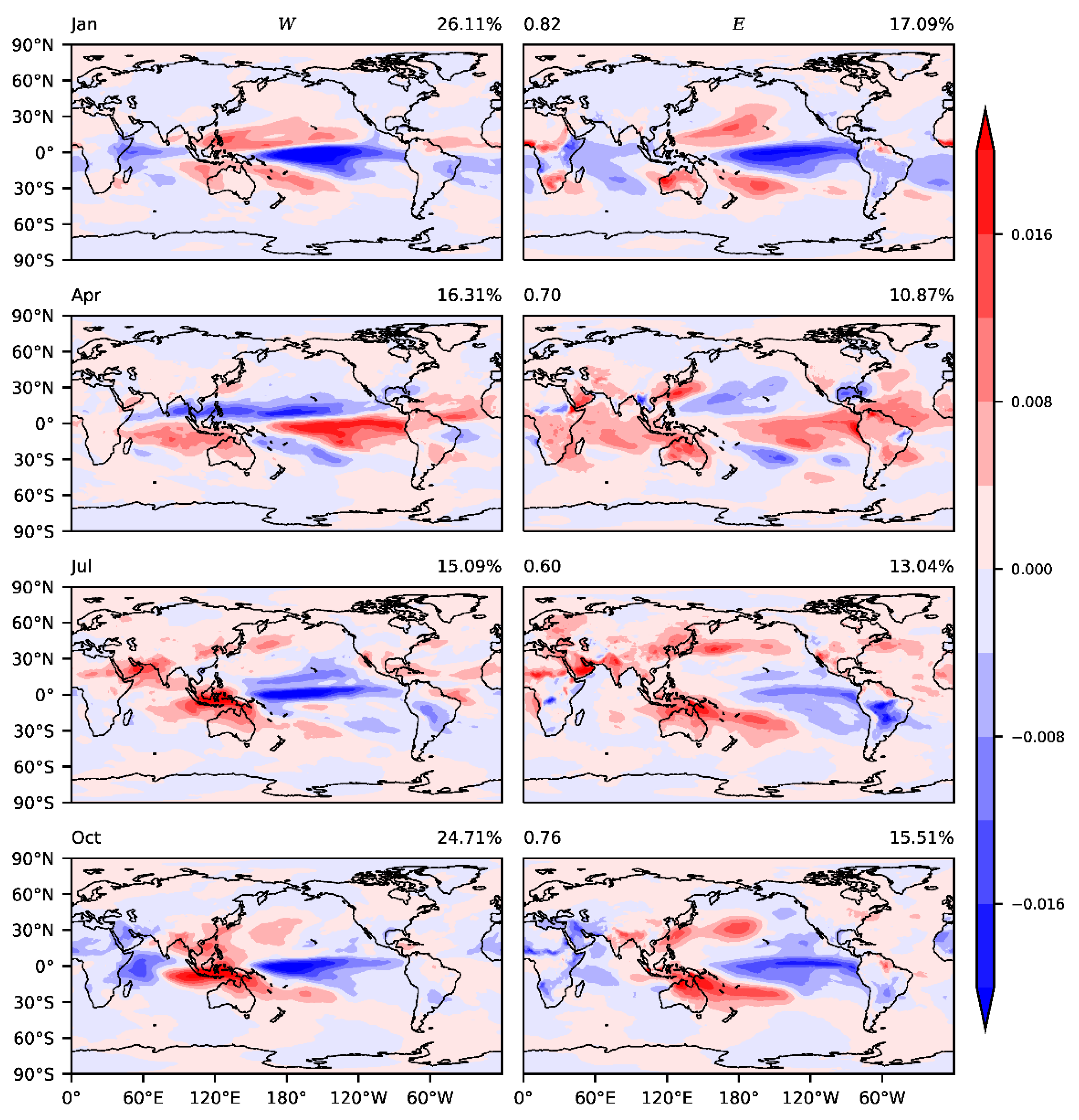
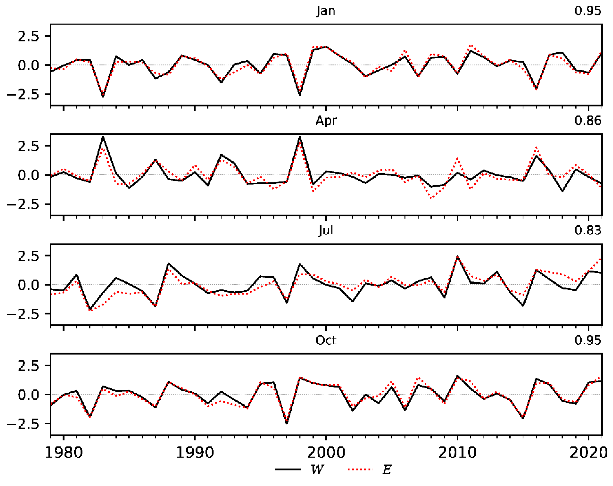
3.3. The Consistency of the First Leading EOF Modes

To further confirm the reliability of the relationship between SVP and PW, the first EOF patterns (EOF 1) of PW and SVP are shown and compared. Figure 9 shows EOF 1 of PW and SVP obtained with the ERA5 dataset (results obtained with JRA55 and NCEP2 are shown in Figures S11 and S12 in the Supplementary Materials). With the Monte Carlo technique, the first three EOFs can be significantly distinguished from the noise. The 0.05 significance level needs the explained variances of the first three modes beyond 2.70%, 2.66%, and 2.65% respectively, with the spatial-temporal resolution (73 × 144 grids and 43 years) used here. There exist ENSO-like patterns, the inverse deviations in Northwest and Mid-to-East Pacific, in all four months, accordant with the result in [8,37]. However, what is mostly important is the similarity of patterns and time series of the two quantities. The result of ERA5 shows that the spatial patterns of the two quantities are quite similar. Relatively more differences exist in the negative value parts of the Tropical Pacific and the Indian Ocean in April. The pattern of SVP in the Pacific is more eastern compared with those of PW in July and October.
The result calculated with JRA55 is similar, while the little divergences between PW and SVP are also over the Tropical Pacific in April and July. What needs attention is that there is a great distinction between the first modes of these two variables in April. After verification, it is confirmed that EOF 1 of PW corresponds well with EOF 2 of SVP. Hence, EOF 1 of SVP in April is replaced by EOF 2 in the result of JRA55.
The differences between spatial patterns of PW and SVP are relatively larger in the result of NCEP2. The distinctions of patterns are obvious in April, July, and October. The negative values of SVP on oceans are visibly weak. Especially in October, not only the is the intensity of the negative center in the Tropical Pacific not so coherent, but there are also some contradictions in the Middle East and Southeast Africa. The spatial correlation coefficient in October is just 0.37, which is much lower than those in other months.
EOF 2 and EOF 3 of the two variables are also compared, and they also correspond well (results are shown in Figures S13–S18 in the Supplementary Materials). The spatial correlation coefficients of the patterns are generally over 0.5 for EOF 2 except in October calculated with NCEP2 (the correlation coefficient is −0.34 and can pass the 0.01 significance level), and those for EOF 3 are generally over 0.4. EOF 3 of PW and SVP calculated with ERA5 is relatively less coherent in January and April, with the spatial correlation coefficient of the patterns being −0.32 and −0.29, respectively. However, because of the long sequence (73 × 144), the correlation coefficients can still pass the 0.01 significance level. Similar to the condition in April in the result of JRA55, EOF 3 of PW is more consistent with EOF 4 of SVP in January in ERA55. Hence, the subgraph of SVP in January in Figure S16 is EOF 4 of it.
As a whole, EOF 1 of PW and SVP obtained with ERA5 and JRA55 datasets is more coherent than that obtained with NCEP2. Even in NCEP2, spatial correlation coefficients of PW and SVP can pass the 0.01 significance level and are larger than 0.66 in January, April, and July. The first three leading modes all show good coherences between PW and SVP. Even the lowest spatial correlation coefficient between the EOF patterns of two variables can still pass the 0.01 significance level.
Corresponding to the consistency of spatial patterns, the time series of SVP and PW obtained with ERA5 almost overlaps in many periods (Figure 10; results calculated with JRA55 and NCEP2 are shown in Figures S19 and S20 in the Supplementary Materials; The time series of EOF 2 and EOF 3 calculated with three dataset are shown in Figures S21–S26 in the Supplementary Materials). The correlation coefficients of the SVP and PW time series are generally over 0.8. As for the NCEP2, the time series with the largest discrepancies exist in October, with a 0.52 correlation coefficient. In October, the time series of SVP is stable with an increasing trend, while the PW is fluctuating.
The time series of EOF 2 and EOF 3 are also examined. The absolute values of correlation coefficients of the corresponding time series are generally over 0.7, and the lowest value is 0.44, which is obtained with the time series of EOF 3 in January calculated with the ERA5 dataset. Corresponding to the relative less consistency of EOF 3 in January and April calculated with ERA5, the time series of EOF 3 in these two months is also less coherent.
Combining the spatial patterns and time series synthetically, the first three EOF leading modes and time series of PW and SVP can correspond well in ERA5 and JRA55. Most contractors exist in the Tropical Indian Ocean and the Tropical Atlantic. Most of the differences in the Pacific are intensity differences. The consistency of the EOF modes of PW and SVP in results further proves the close relationship between them in interannual and long-term variations. It is a complement to the statistical basis of using the variations of SVP to represent those of PW, or the reverse.

4. Summary and Discussion

Because of the deficiency of high-altitude observations and the internal physical relation of PW and SVP, the linkage between them has been researched for some decades. The time scales mainly researched are the daily and annual cycles. Whether the linkage is reliable everywhere at interannual and long-term variations is examined in this paper. With the examination, we can reveal the areas where it is difficult to obtain an efficient empirical equation between PW and SVP and the regions where the variations of SVP and PW can well reflect each other.
Results show that the interannual variations of monthly mean PW and SVP are strongly correlated in most areas, with correlation coefficients generally over 0.8. Correlations at high latitudes are stronger than those at low latitudes, and correlations in winter are stronger than those in summer. The insignificant correlations just exist over tropical oceans and some high-altitude areas in the Northern Hemisphere in Boreal Summer.
The vertical profiles of specific humidity and vertical velocity in weak and strong correlation regions are compared to figure out the reasons for the weaker correlations. Over the ocean, the weak correlation could be mainly due to the unstable and strong convection. On land, the weak correlation is associated with the extreme drought near the surface. Under the drought conditions, the downward motions in these areas probably break the linear relationship. There is only a little moisture, so the effects of vertical movements are relatively more destructive.
The long-term trends of SVP and PW are also analyzed. In a large number of areas besides some areas of the Tropical Indian Ocean and Middle Africa, the long-term trends of SVP can well reflect those of PW. Three datasets exhibit a common characteristic that the trends of SVP in North Eurasia are stronger than those of PW. The trends of SVP in high-latitude areas of Eurasia are stronger than those of PW, indicating that the upward movements are attenuated, and evaporation is enhanced along with warming. The vapor convergence at high levels may be weaker along with the weakening of circulations.
As a whole, the variations of SVP and PW are consistent in vast areas, especially in ERA5. At the interannual scale, the variation in PW can be reflected by that of SVP in most extratropical areas except in July. It is feasible to use the interannual variation in SVP to reflect that of PW in extratropical areas except in July, but researchers must be careful when performing this in the Tropical West Pacific and the Tropical Atlantic. In these areas, it should be relatively hard to establish an effective empirical equation between PW and SVP. On the long-term scale, the trend direction of PW can be well reflected by that of SVP, except in the Tropical Indian Ocean east to Africa and the Tropical Atlantic east to South America. The weaker correlations are mainly caused by the vertical movements which can cause the large fluctuation of specific humidity at middle levels and adjust the profiles of specific humidity, while it also means that the atmosphere is not in hydrostatic equilibrium.
The close linkage between SVP and PW is an extension of another study by us [39]. The response of SVP to surface temperature is studied in another part of our work. With the linkage between PW and SVP, the response characteristics of column WV content can be reflected by those of SVP. In addition, it provides a brief description of where the PW can be well regressed with SVP, or the other way around. Because the specific values of trends, interannual correlation coefficients, and EOF modes differ among different datasets, some areas with large discrepancies need more accurate observations to be verified, such as the Indian Ocean and the east coast of South America. Perhaps using SVP at several grids to estimate PW (or in reverse order) or using several surface variables to estimate PW will achieve a better effect. It is worth trying, and it may be suitable to combine some neural network methods.

Supplementary Materials

The following supporting information can be downloaded at: https://www.mdpi.com/article/10.3390/atmos13091350/s1, Figure S1: Maps of correlation coefficients of PW and SVP (The dataset used is JRA55). The correlation coefficients in shaded areas cannot pass the 0.05 significance level. Blue and red squares are strong and weak correlation areas respectively selected to show the vertical profiles, Figure S2: Maps of correlation coefficients of PW and SVP (The dataset used is NCEP2). The correlation coefficients in shaded areas cannot pass the 0.05 significance level. Blue and red squares are strong and weak correlation areas respectively selected to show the vertical profiles, Figure S3: The curves of normalized PW and SVP in strong correlation areas on land (blue squares in January in Figure 1, Figure S1, and Figure S2), Figure S4: The curves of normalized PW and SVP in weak correlation areas on land (red squares in January in Figure 1, Figure S1, and Figure S2), Figure S5: The curves of normalized PW and SVP in strong correlation areas over the oceans (blue squares in July in Figure 1, Figure S1, and Figure S2), Figure S6: The curves of normalized PW and SVP in weak correlation areas (red squares in July in Figure 1, Figure 2 and Figure 3) over the oceans, Figure S7: The long-term trends of PW (the left column, unit: kg∙m−2/10 yr) and SVP (the right column, unit: hPa/10 yr) in four months calculated with the JRA55 dataset. The rows from top to bottom respond to January, April, July, and October respectively. Trends in the shaded areas can reach the 0.05 significance level, Figure S8: The long-term trends of PW (the left column, unit: kg∙m−2/10 yr) and SVP (the right column, unit: hPa/10 yr) in four months calculated with the NCEP2 dataset. The rows from top to bottom respond to January, April, July, and October respectively. Trends in the shaded areas can reach the 0.05 significance level, Figure S9: The time series of normalized global areal-weighted averages of 2 m temperature (T), PW (W), and SVP (E) in January (a), April (b), July (c), and October (d) calculated with JRA55 datasets. The four numbers at the top-right of subgraphs are the correlation coefficient between PW and SVP and Sen’s slope value of three elements (T, W, and E in sequence; units: K/10 yr, kg∙m−2/10 yr, and hPa/10 yr), separately, Figure S10: The time series of normalized global areal-weighted averages of 2 m temperature (T), PW (W), and SVP (E) in January (a), April (b), July (c), and October (d) calculated with NCEP2 datasets. The four numbers at the top-right of subgraphs are the correlation coefficient between PW and SVP and Sen’s slope value of three elements (T, W, and E in sequence; units: K/10 yr, kg∙m−2/10 yr, and hPa/10 yr), separately, Figure S11: The first EOF modes of PW (left) and SVP (right) calculated with JRA55. (The rows from top to bottom correspond to January, April, July, and October respectively. The percentages at the top-right of subgraphs are fractional mode variances corresponding to PW and SVP. The numbers at the upper-left corners of graphs in the right column are spatial correlation coefficients of the first modes of PW and SVP), Figure S12: The first EOF modes of PW (left) and SVP (right) calculated with NCEP2. (The rows from top to bottom correspond to January, April, July, and October respectively. The percentages at the top-right of subgraphs are fractional mode variances corresponding to PW and SVP. The numbers at the upper-left corners of graphs in the right column are spatial correlation coefficients of the first modes of PW and SVP), Figure S13: The second EOF modes of PW (left) and SVP (right) calculated with ERA5. (The rows from top to bottom correspond to January, April, July, and October respectively. The percentages at the top-right of subgraphs are fractional mode variances corresponding to PW and SVP. The numbers at the upper-left corners of graphs in the right column are spatial correlation coefficients of the first modes of PW and SVP.), Figure S14: The second EOF modes of PW (left) and SVP (right) calculated with JRA55. (The rows from top to bottom correspond to January, April, July, and October respectively. The percentages at the top-right of subgraphs are fractional mode variances corresponding to PW and SVP. The numbers at the upper-left corners of graphs in the right column are spatial correlation coefficients of the first modes of PW and SVP.), Figure S15: The second EOF modes of PW (left) and SVP (right) calculated with ncep2. (The rows from top to bottom correspond to January, April, July, and October respectively. The percentages at the top-right of subgraphs are fractional mode variances corresponding to PW and SVP. The numbers at the upper-left corners of graphs in the right column are spatial correlation coefficients of the first modes of PW and SVP.), Figure S16: The third EOF modes of PW (left) and SVP (right) calculated with ERA5. (The rows from top to bottom correspond to January, April, July, and October respectively. The percentages at the top-right of subgraphs are fractional mode variances corresponding to PW and SVP. The numbers at the upper-left corners of graphs in the right column are spatial correlation coefficients of the first modes of PW and SVP.), Figure S17: The third EOF modes of PW (left) and SVP (right) calculated with JRA55. (The rows from top to bottom correspond to January, April, July, and October respectively. The percentages at the top-right of subgraphs are fractional mode variances corresponding to PW and SVP. The numbers at the upper-left corners of graphs in the right column are spatial correlation coefficients of the first modes of PW and SVP.)., Figure S18: The third EOF modes of PW (left) and SVP (right) calculated with NCEP2. (The rows from top to bottom correspond to January, April, July, and October respectively. The percentages at the top-right of subgraphs are fractional mode variances corresponding to PW and SVP. The numbers at the upper-left corners of graphs in the right column are spatial correlation coefficients of the first modes of PW and SVP.), Figure S19: The principal components of EOF 1 of PW and SVP were calculated with the JRA55 dataset (scaled to unit variance). The numbers at the top-right of subgraphs are correlation coefficients of two curves, Figure S20: The principal components of EOF 1 of PW and SVP were calculated with the NCEP2 dataset (scaled to unit variance). The numbers at the top-right of subgraphs are correlation coefficients of two curves, Figure S21: The principal components of EOF 2 of PW and SVP were calculated with the ERA5 dataset (scaled to unit variance). The numbers at the top-right of subgraphs are correlation coefficients of two curves, Figure S22: The principal components of EOF 2 of PW and SVP were calculated with the JRA55 dataset (scaled to unit variance). The numbers at the top-right of subgraphs are correlation coefficients of two curves, Figure S23: The principal components of EOF 2 of PW and SVP were calculated with the NCEP2 dataset (scaled to unit variance). The numbers at the top-right of subgraphs are correlation coefficients of two curves, Figure S24: The principal components of EOF 3 of PW and SVP were calculated with the ERA5 dataset (scaled to unit variance). The numbers at the top-right of subgraphs are correlation coefficients of two curves, Figure S25: The principal components of EOF 3 of PW and SVP were calculated with the JRA55 dataset (scaled to unit variance). The numbers at the top-right of subgraphs are correlation coefficients of two curves, Figure S26: The principal components of EOF 3 of PW and SVP were calculated with the NCEP2 dataset (scaled to unit variance). The numbers at the top-right of subgraphs are correlation coefficients of two curves.

Author Contributions

Conceptualization, J.H. and E.L.; methodology, E.L.; software, J.H.; validation, J.H.; formal analysis, J.H. and E.L.; investigation, J.H.; resources, J.H.; data curation, J.H.; writing—original draft preparation, J.H.; writing—review and editing, J.H. and E.L.; visualization, J.H.; supervision, E.L.; project administration, E.L.; funding acquisition, E.L. All authors have read and agreed to the published version of the manuscript.

Funding

This study was supported by the National Natural Science Foundation of China (Grant Number: 41991281), the National Key Research and Development Program of China (Grant Number: 2018YFC1507704), and the Priority Academic Program Development of Jiangsu Higher Education Institutions (PAPD).

Institutional Review Board Statement

Not applicable.

Informed Consent Statement

Not applicable.

Data Availability Statement

Datasets analyzed during the current study include ERA5, JRA55, and NCEP2. The ERA5 dataset is available in the Copernicus Climate Change Service Climate Date Store (https://cds.climate.copernicus.eu/#!/search?text=ERA5&type=dataset, accessed on 1 July 2022), provided by ECMWF. The JRA55 dataset is available in the Research Data Archive, managed by NCAR (https://rda.ucar.edu/datasets/ds628.1/#!access, accessed on 1 July 2022), provided by JMA. The NCEP2 dataset is available in the Physical Sciences Laboratory (PSL) (https://psl.noaa.gov/data/gridded/data.ncep.reanalysis2.html, accessed on 1 July 2022), provided by the NOAA/OAR/ESRL PSL.

Acknowledgments

The introduction of EOF analysis is cited from National Center for Atmospheric Research Staff (Eds). Last modified 22 July 2013. “The Climate Data Guide: Empirical Orthogonal Function (EOF) Analysis and Rotated EOF Analysis.” retrieved from https://climatedataguide.ucar.edu/climate-data-tools-and-analysis/empirical-orthogonal-function-eof-analysis-and-rotated-eof-analysis, accessed on 1 July 2022.

Conflicts of Interest

The authors declare no conflict of interest.

References

  1. Stewart, R.E.; Crawford, R.W.; Leighton, H.G.; Marsh, P.; Strong, G.S.; Moore, G.W.K.; Ritchie, H.; Rouse, W.R.; Soulis, E.D.; Kochtubajda, B. The Mackenzie GEWEX Study: The Water and Energy Cycles of a Major North American River Basin. Bull. Am. Meteorol. Soc. 1998, 79, 2665–2683. [Google Scholar] [CrossRef]
  2. Semmler, T.; Jacob, D.; Schlünzen, K.H.; Podzun, R. The Water and Energy Budget of the Arctic Atmosphere. J. Clim. 2005, 18, 2515–2530. [Google Scholar] [CrossRef]
  3. Trenberth, K.E.; Fasullo, J. Regional Energy and Water Cycles: Transports from Ocean to Land. J. Clim. 2013, 26, 7837–7851. [Google Scholar] [CrossRef]
  4. Mathew, S.S.; Kumar, K.K. On the role of precipitation latent heating in modulating the strength and width of the Hadley circulation. Arch. Meteorol. Geophys. Bioclimatol. Ser. B 2018, 136, 661–673. [Google Scholar] [CrossRef]
  5. Hao, J.; Lu, E. The quantitative comparison of contributions from vapour and temperature to midsummer precipitation in China under the influence of spring heat source over Tibet Plateau. Int. J. Clim. 2021, 42, 1754–1766. [Google Scholar] [CrossRef]
  6. Zhou, T.-J.; Yu, R.-C. Atmospheric water vapor transport associated with typical anomalous summer rainfall patterns in China. J. Geophys. Res. Atmos. 2005, 110. [Google Scholar] [CrossRef]
  7. Rädel, G.; Shine, K.P.; Ptashnik, I.V. Global radiative and climate effect of the water vapour continuum at visible and near-infrared wavelengths. Q. J. R. Meteorol. Soc. 2014, 141, 727–738. [Google Scholar] [CrossRef]
  8. Wang, Y.; Zhang, Y.; Fu, Y.; Li, R.; Yang, Y.-J. A climatological comparison of column-integrated water vapor for the third-generation reanalysis datasets. Sci. China Earth Sci. 2015, 59, 296–306. [Google Scholar] [CrossRef]
  9. Cady-Pereira, K.; Shephard, M.; Turner, D.; Mlawer, E.; Clough, S.; Wagner, T. Improved daytime column-integrated precipitable WV from Vaisala radiosonde humidity sensors. J. Atmos. Ocean. Technol. 2008, 25, 873–883. [Google Scholar] [CrossRef]
  10. Durre, I.; Williams, C.N.; Yin, X.; Vose, R.S. Radiosonde-based trends in precipitable water over the Northern Hemisphere: An update. J. Geophys. Res. Earth Surf. 2009, 114. [Google Scholar] [CrossRef]
  11. Wang, J.X.L.; Gaffen, D.J. Late-Twentieth-Century Climatology and Trends of Surface Humidity and Temperature in China. J. Clim. 2001, 14, 2833–2845. [Google Scholar] [CrossRef]
  12. Dai, A. Recent Climatology, Variability, and Trends in Global Surface Humidity. J. Clim. 2006, 19, 3589–3606. [Google Scholar] [CrossRef]
  13. Willett, K.M.; Jones, P.; Gillett, N.P.; Thorne, P. Recent Changes in Surface Humidity: Development of the HadCRUH Dataset. J. Clim. 2008, 21, 5364–5383. [Google Scholar] [CrossRef]
  14. Isaac, V.; Van Wijngaarden, W. Surface WV pressure and temperature trends in North America during 1948–2010. J. Clim. 2012, 25, 3599–3609. [Google Scholar] [CrossRef]
  15. Wallace, J.M.; Hobbs, P.V. Atmospheric Science: An Introductory Survey; Elsevier: Amsterdam, The Netherlands, 2006; 483p. [Google Scholar]
  16. Lu, E.; Zeng, X. Understanding different precipitation seasonality regimes from WV and temperature fields: Case studies. Geophys. Res. Lett. 2005, 32, 1154–1158. [Google Scholar] [CrossRef]
  17. Lu, E. Understanding the effects of atmospheric circulation in the relationships between water vapor and temperature through theoretical analyses. Geophys. Res. Lett. 2007, 34. [Google Scholar] [CrossRef]
  18. Reber, E.E.; Swope, J.R. On the Correlation of the Total Precipitable Water in a Vertical Column and Absolute Humidity at the Surface. J. Appl. Meteorol. 1972, 11, 1322–1325. [Google Scholar] [CrossRef]
  19. Viswanadham, Y. The Relationship between Total Precipitable Water and Surface Dew Point. J. Appl. Meteorol. 1981, 20, 3–8. [Google Scholar] [CrossRef]
  20. Liu, W.T. Statistical Relation between Monthly Mean Precipitable Water and Surface-Level Humidity over Global Oceans. Mon. Weather Rev. 1986, 114, 1591–1602. [Google Scholar] [CrossRef]
  21. Hsu, S.A.; Blanchard, B.W. The relationship between total precipitable water and surface-level humidity over the sea surface: A further evaluation. J. Geophys. Res. Earth Surf. 1989, 94, 14539–14545. [Google Scholar] [CrossRef]
  22. Dostalek, J.F.; Schmit, T.J. Total Precipitable Water Measurements from GOES Sounder Derived Product Imagery. Weather Forecast. 2001, 16, 573–587. [Google Scholar] [CrossRef]
  23. Deeter, M.N. A new satellite retrieval method for precipitable water vapor over land and ocean. Geophys. Res. Lett. 2007, 34. [Google Scholar] [CrossRef]
  24. Radhakrishna, B.; Fabry, F.; Braun, J.J.; Van Hove, T. Precipitable Water from GPS over the Continental United States: Diurnal Cycle, Intercomparisons with NARR, and Link with Convective Initiation. J. Clim. 2015, 28, 2584–2599. [Google Scholar] [CrossRef]
  25. Torri, G.; Adams, D.K.; Wang, H.; Kuang, Z. On the diurnal cycle of GPS-derived precipitable WV over Sumatra. J. Atmos. Sci. 2019, 76, 3529–3552. [Google Scholar] [CrossRef]
  26. Zveryaev, I.I.; Chu, P.-S. Recent climate changes in precipitable water in the global tropics as revealed in National Centers for Environmental Prediction/National Center for Atmospheric Research reanalysis. J. Geophys. Res. Atmos. 2003, 108, ACL6.1–ACL6.10. [Google Scholar] [CrossRef]
  27. Ssenyunzi, R.C.; Oruru, B.; D’ujanga, F.M.; Realini, E.; Barindelli, S.; Tagliaferro, G.; von Engeln, A.; van de Giesen, N. Performance of ERA5 data in retrieving Precipitable Water Vapour over East African tropical region. Adv. Space Res. 2020, 65, 1877–1893. [Google Scholar] [CrossRef]
  28. Maghrabi, A.; Al Dajani, H. Estimation of precipitable water vapour using vapour pressure and air temperature in an arid region in central Saudi Arabia. J. Assoc. Arab Univ. Basic Appl. Sci. 2013, 14, 45–49. [Google Scholar] [CrossRef]
  29. Chadwick, R.; Good, P.; Willett, K. A Simple Moisture Advection Model of Specific Humidity Change over Land in Response to SST Warming. J. Clim. 2016, 29, 7613–7632. [Google Scholar] [CrossRef]
  30. Gaffen, D.J.; Elliott, W.P.; Robock, A. Relationships between tropospheric WV and surface temperature as observed by radiosondes. Geophys. Res. Lett. 1992, 19, 1839–1842. [Google Scholar] [CrossRef]
  31. Sun, D.-Z.; Held, I.M. A comparison of modeled and observed relationships between interannual variations of WV and temperature. J. Clim. 1996, 9, 665–675. [Google Scholar] [CrossRef]
  32. Bauer, M.; Del Genio, A.D.; Lanzante, J.R. Observed and Simulated Temperature–Humidity Relationships: Sensitivity to Sampling and Analysis. J. Clim. 2002, 15, 203–215. [Google Scholar] [CrossRef]
  33. Mears, C.A.; Santer, B.D.; Wentz, F.J.; Taylor, K.E.; Wehner, M.F. Relationship between temperature and precipitable water changes over tropical oceans. Geophys. Res. Lett. 2007, 34. [Google Scholar] [CrossRef]
  34. Laine, A.; Nakamura, H.; Nishii, K.; Miyasaka, T. A diagnostic study of future evaporation changes projected in CMIP5 climate models. Clim. Dyn. 2014, 42, 2745–2761. [Google Scholar] [CrossRef]
  35. Trenberth, K.E.; Fasullo, J.; Smith, L. Trends and variability in column-integrated atmospheric WV. Clim. Dyn. 2005, 24, 741–758. [Google Scholar] [CrossRef]
  36. Chung, E.-S.; Soden, B.; Sohn, B.J.; Shi, L. Upper-tropospheric moistening in response to anthropogenic warming. Proc. Natl. Acad. Sci. USA 2014, 111, 11636–11641. [Google Scholar] [CrossRef]
  37. Zhang, Y.; Xu, J.; Yang, N.; Lan, P. Variability and Trends in Global Precipitable Water Vapor Retrieved from COSMIC Radio Occultation and Radiosonde Observations. Atmosphere 2018, 9, 174. [Google Scholar] [CrossRef]
  38. Schröder, M.; Lockhoff, M.; Shi, L.; August, T.; Bennartz, R.; Brogniez, H.; Calbet, X.; Fell, F.; Forsythe, J.; Gambacorta, A.; et al. The GEWEX Water Vapor Assessment: Overview and Introduction to Results and Recommendations. Remote Sens. 2019, 11, 251. [Google Scholar] [CrossRef]
  39. Hao, J.; Lu, E. Variation of Relative Humidity as Seen through Linking Water Vapor to Air Temperature: An Assessment of Interannual Variations in the Near-Surface Atmosphere. Atmosphere 2022, 13, 1171. [Google Scholar] [CrossRef]
  40. Shi, L.; Schreck, C.; Schröder, M. Assessing the Pattern Differences between Satellite-Observed Upper Tropospheric Humidity and Total Column Water Vapor during Major El Niño Events. Remote Sens. 2018, 10, 1188. [Google Scholar] [CrossRef]
  41. Smith, T.M.; Arkin, P.A. Improved Historical Analysis of Oceanic Total Precipitable Water. J. Clim. 2015, 28, 3099–3121. [Google Scholar] [CrossRef]
  42. Wang, J.; Dai, A.; Mears, C. Global Water Vapor Trend from 1988 to 2011 and Its Diurnal Asymmetry Based on GPS, Radiosonde, and Microwave Satellite Measurements. J. Clim. 2016, 29, 5205–5222. [Google Scholar] [CrossRef]
  43. Hersbach, H.; Bell, B.; Berrisford, P.; Hirahara, S.; Horanyi, A.; Muñoz-Sabater, J.; Nicolas, J.; Peubey, C.; Radu, R.; Schepers, D.; et al. The ERA5 global reanalysis. Q. J. R. Meteorol. Soc. 2020, 146, 1999–2049. [Google Scholar] [CrossRef]
  44. Kanamitsu, M.; Ebisuzaki, W.; Woollen, J.; Yang, S.-K.; Hnilo, J.J.; Fiorino, M.; Potter, G.L. NCEP–DOE AMIP-II Reanalysis (R-2). Bull. Am. Meteorol. Soc. 2002, 83, 1631–1644. [Google Scholar] [CrossRef]
  45. Kobayashi, S.; Ota, Y.; Harada, Y.; Ebita, A.; Moriya, M.; Onoda, H.; Onogi, K.; Kamahori, H.; Kobayashi, C.; Endo, H.; et al. The JRA-55 Reanalysis: General Specifications and Basic Characteristics. J. Meteorol. Soc. Jpn. Ser. II 2015, 93, 5–48. [Google Scholar] [CrossRef]
  46. Alduchov, O.A.; Eskridge, R.E. Improved Magnus Form Approximation of Saturation Vapor Pressure. J. Appl. Meteorol. 1996, 35, 601–609. [Google Scholar] [CrossRef]
  47. Duhan, D.; Pandey, A. Statistical analysis of long term spatial and temporal trends of precipitation during 1901–2002 at Madhya Pradesh, India. Atmos. Res. 2013, 122, 136–149. [Google Scholar] [CrossRef]
  48. Jain, S.K.; Kumar, V. Trend analysis of rainfall and temperature data for India. Curr. Sci. 2012, 102, 37–49. [Google Scholar]
  49. Mann, H.B. Nonparametric tests against trend. Econometrica 1945, 13, 245–259. [Google Scholar] [CrossRef]
  50. Kendall, M.G. Rank Correlation Methods; Charles Grifin: London, UK, 1970; 202p. [Google Scholar]
  51. Mondal, A.; Kundu, S.; Mukhopadhyay, A. Rainfall trend analysis by Mann-Kendall test: A case study of north-eastern part of Cuttack district, Orissa. Int. J. Geol. Earth Environ. Sci. 2012, 2, 70–78. [Google Scholar]
  52. Hamed, K.H.; Rao, A.R. A modified Mann-Kendall trend test for autocorrelated data. J. Hydrol. 1998, 204, 182–196. [Google Scholar] [CrossRef]
  53. Sen, P.K. Estimates of the regression coefficient based on Kendall’s tau. J. Am. Stat. Assoc. 1968, 63, 1379–1389. [Google Scholar] [CrossRef]
  54. Pal, A.B.; Khare, D.; Mishra, P.K.; Singh, L. Trend analysis of rainfall, temperature and runoff data: A case study of Rangoon watershed in Nepal. Int. J. Stud. Res. Technol. Manag. 2017, 5, 21–38. [Google Scholar] [CrossRef]
  55. Schwing, F.; Murphree, T.; Green, P. The Northern Oscillation Index (NOI): A new climate index for the northeast Pacific. Prog. Oceanogr. 2002, 53, 115–139. [Google Scholar] [CrossRef]
  56. Overland, J.E.; Preisendorfer, R.W. A Significance Test for Principal Components Applied to a Cyclone Climatology. Mon. Weather Rev. 1982, 110, 699–706. [Google Scholar] [CrossRef]
  57. Peixoto, J.P.; Oort, A.H. Physics of Climate; American Institute of Physics: New York, NY, USA, 1992; 520p. [Google Scholar]
Figure 1. Maps of correlation coefficients of PW and SVP (the dataset used is ERA5). The correlation coefficients in shaded areas cannot pass the 0.05 significance level. Blue and red squares are strong and weak correlation areas, respectively, selected to show the vertical profiles.
Atmosphere 13 01350 g001
Figure 2. The vertical profiles of specific humidity in strong and weak correlation continental areas. (unit: g∙kg−1). The shaded areas are the range of one standard deviation. (a) ERA5 datasets, (b) JRA55 datasets, and (c) NCEP2 datasets. The specific areas chosen are squared in Figure 1, Figures S1 and S2, correspondingly (Figures S1 and S2 are in the Supplementary Materials). Because the land surface pressure is around 940 hPa, the lowest level shown is 925 hPa).
Atmosphere 13 01350 g002
Figure 3. The contents are similar to Figure 2, but the areas squared are oceanic areas. (a) ERA5 datasets, (b) JRA55 datasets, and (c) NCEP2 datasets.
Atmosphere 13 01350 g003
Figure 4. The vertical profiles of vertical velocity in strong and weak correlation continental areas. (unit: Pa∙s−1). The shaded areas are the range of one standard deviation. (a) ERA5 datasets, (b) JRA55 datasets, and (c) NCEP2 datasets. The specific areas chosen are squared in Figure 1, Figures S1 and S2, correspondingly. Because the land surface pressure is around 940 hPa, the lowest level shown is 925 hPa).
Atmosphere 13 01350 g004
Figure 5. The contents are similar to Figure 4, but the areas squared are oceanic areas. (a) ERA5 datasets, (b) JRA55 datasets, and (c) NCEP2 datasets.
Atmosphere 13 01350 g005
Figure 6. The long-term trends of PW (the left column, unit: kg∙m−2/10 yr) and SVP (the right column, unit: hPa/10 yr) in four months calculated with the ERA5 dataset. The rows from top to bottom correspond to January, April, July, and October, respectively. Trends in the shaded areas can reach the 0.05 significance level.
Atmosphere 13 01350 g006
Figure 7. Scatter plots of PW and SVP trends at grids in four months. Each dot is a grid. The columns from left to right correspond to ERA5, JRA55, and NCEP2. The rows from top to bottom correspond to four months. The black line is the linear regression line of PW and SVP. The grey line is the y = x line. R is the spatial correlation coefficient of PW and SVP. The equation in the right bottom corner is the regression equation.
Atmosphere 13 01350 g007
Figure 8. The time series of normalized global areal-weighted averages of 2 m temperature (T), PW (W), and SVP (E) in January (a), April (b), July (c), and October (d) calculated with ERA5 datasets. The four numbers at the top-right of subgraphs are the correlation coefficient between PW and SVP and Sen’s slope value of three elements (T, W, and E in sequence; units: K/10 yr, kg∙m−2/10 yr, and hPa/10 yr), separately.
Atmosphere 13 01350 g008
Figure 9. The first EOF (EOF1) modes of PW (left) and SVP (right) calculated with ERA5. The rows from top to bottom correspond to January, April, July, and October, respectively. The percentages at the top-right of subgraphs are fractional mode variances corresponding to PW and SVP. The numbers at the upper-left corners of graphs in the right column are spatial correlation coefficients of the first modes of PW and SVP.
Atmosphere 13 01350 g009
Figure 10. The principal component time series (PCs) of EOF 1 of PW and SVP was calculated with the ERA5 dataset (scaled to unit variance). The numbers at the top-right of subgraphs are correlation coefficients of two curves.
Atmosphere 13 01350 g010
Table 1. The variables directly downloaded from the servers. The variables that need calculation are in brackets, and the variable in each pair of brackets is calculated with the corresponding variable out of the brackets.
DatasetsSingle Level VariablesPressure Level Variables
ERA52 m temperature (saturated SVP)
2 m dewpoint temperature (SVP)
precipitable water
vertical velocity
temperature (saturated SVP)
specific humidity
JRA55
NCEP2relative humidity (specific humidity)
Publisher’s Note: MDPI stays neutral with regard to jurisdictional claims in published maps and institutional affiliations.

