Abstract
CO2 emissions from fossil energy have caused global climate problems and threatened human survival. However, there are few studies on the spatiotemporal distribution and driving factors of carbon emissions. This paper takes the Yangtze River Delta (YRD) urban agglomeration as the research object and analyzes the spatiotemporal heterogeneity of carbon dioxide emissions and their driving factors from 2000 to 2017. First, a series of preprocessing, such as resample, interpolation, and image clipping, are conducted on the CO2 emission data and nighttime light remote sensing images. Second, the dynamic time wrapping (DTW) and hierarchical clustering algorithms were involved in manipulating the CO2 emission data. Consequently, the cities’ and CO2 emissions’ time series were classified into four categories and three stages separately. Finally, the geographical detector model (GDM) and geographical and temporal weighted regression (GTWR) are coupled to evaluate the spatiotemporal heterogeneity and quantify the driving factors. The results show the following: (1) The spatiotemporal distribution of CO2 emissions has spatial consistency from 2000 to 2017. High-emission areas are concentrated in economically developed areas such as Shanghai, Suzhou, and Wuxi. The results are consistent with previous research. (2) Regional aggregation is a revealed new trend. CO2 emissions in the target urban areas are gradually converging into economic center cities and diverse class cities, e.g., Shanghai and Ningbo. (3) In cities of different economic development levels, the driving factors of CO2 emissions are different. The secondary sector and urban infrastructure dominate in the early stages of developed cities. On top of that, the influence of the tertiary industry is more significant in the later development stages. According to the results, in the urban development process, humans should not only pursue the increase in speed but also pay attention to the negative impact of the economic development process on the ecological environment. Besides, since the spatiotemporal characteristics and dominant factors of urban carbon emissions are different in each stage of development, the formulation of carbon reduction policies should be associated with urban features.
1. Introduction
As a major greenhouse gas, CO2 has been proven to be the major contributor to global warming. The World Meteorological Organization states that the total climate warming effect of greenhouse gases has increased by 43% since 1990, 82% of which is caused by CO2 [1]. Most of the CO2 emissions are from human economic production and daily life [2]. The World Meteorological Organization’s 2017 Greenhouse Gas Bulletin reported that the concentrations of CO2 emissions in the atmosphere surged at a record-breaking speed in 2016 to the highest level in 800,000 years [3]. This is an unprecedented sudden change in the atmosphere and highlights the urgency of CO2 management [4]. Therefore, reducing carbon emissions and achieving a low-carbon economy have become critical issues worldwide.
China is one of the major carbon-emitting countries in the world [5]. According to statistics, 28% of global carbon emissions came from China in 2013; meanwhile, China’s per capita emissions exceeded those of the European Union for the first time [6]. To slow down the growth of carbon emissions, China is targeting peak carbon dioxide emissions by 2030 and carbon neutrality by the year 2060 [7].
Aiming at the measurement of carbon dioxide emissions from energy consumption, the quantitative evaluation of spatiotemporal variation, as well as the identification and quantification of influencing factors, numerous scholars have conducted relevant studies (see Table 1). For instance, Wang and He found a significant positive correlation between economic growth and carbon emissions [8,9]. As the prominent gathering place of human production and life, cities are the centers of economic activity and the central area of energy consumption and carbon emissions. According to the estimation of related scholars, 35 large cities in China account for 40% of the total carbon emissions in this country [5]. Therefore, it is vital to understand the spatial and temporal distribution of carbon emissions and their influencing factors in different periods in Chinese cities, especially in large urban agglomerations with more developed economies. This step is important for analyzing the structure and variability trends of carbon emissions in cities at different development levels and formulating energy conservation and emission reduction policies. Moreover, it is an essential theoretical basis for achieving the goals of carbon peaking and carbon neutrality.

Table 1.
Research on low carbon development.
Current studies related to CO2 emissions have mainly focused on the provincial scale. For example, Wang et al. [14] estimated the carbon emissions of 30 provinces using energy consumption data from provincial statistical bureaus in China. They found that the emission level in eastern China was significantly higher than in central and western China. On the other hand, at the prefecture-level city scale, only a few local statistical bureaus provide detailed energy consumption data. It is challenging to ensure the long-term continuity of the data, so it is difficult to reveal the spatial variability of carbon emissions fully. From recent developments in remote sensing of nighttime lights, nighttime light images are an excellent data source for monitoring the intensity of human activity. It provides an essential basis for the quantitative estimation and spatialization of socioeconomic and environmental indicators, including carbon emissions. Numerous scholars have calibrated and fused DMSP-OLS and NPP-VIIRS data to extend the time series length of nighttime light data to construct carbon emission estimation models from provincial [6], urban agglomeration [21], city [22], and county scales [23]. These studies prove that nighttime light data is more accurate for carbon emission estimation. However, it is challenging for researchers to correct these two sets of data across sensors to construct a high-quality long-time series of nighttime light data.
In terms of carbon emission estimation methods, there are mainly Intergovernmental Panel on Climate Change (IPCC) estimation methods [24,25], field measurement methods [26,27], and model estimation methods [28,29]. Field measurement methods and model estimation methods can obtain high-accuracy carbon emission data but have high costs for practical implementation. The IPCC estimation method is a calculation method based on energy consumption statistics. This method has low data requirements, simple and convenient calculations, and strong applicability. Therefore, more and more scholars use the IPCC estimation method to estimate carbon emissions. However, since the data obtained by the IPCC estimation method may have inevitable errors, the IPCC estimation method needs to be combined with the night light data to correct the obtained city-level energy carbon emission data.
In the study of the spatiotemporal heterogeneity of CO2 driving indicators, the primary methods used are the Logarithmic Mean Divisia Index (LMDI)method [30,31], multiple linear regression models [32,33], geographically weighted models [34,35], and spatial econometric models [36,37]. For example, Wang et al. [8] used LMDI to analyze data from 1957–2000 in China and found that economic growth increases CO2 emissions. Wang et al. [38] derived that private vehicle possession, gross national product, and energy consumption positively affect carbon emissions by constructing a geographically weighted regression model. Shu et al. [32] used a multiple linear regression model to spatially decompose the carbon emissions from road traffic and concluded that the correlation between road density and carbon emissions was highly significant. Based on a spatial panel econometric model, He et al. [9] completed a significant positive correlation between economic growth and carbon emissions. These methods have their applicability. For example, the linear regression model only focuses on the fitted coefficients of the independent variables. It does not consider that the relationship between the independent and dependent variables varies with spatial location. Although the geographically weighted regression model makes up for the shortcomings of the linear regression model, the method still has limitations in the case of multicollinearity among the independent variables. Compared with multiple linear and geographically weighted regression, the Geographical Detector Model can better consider the effects of multicollinearity and spatial location. The spatiotemporal Geographical and Temporal Weighted Regression can well solve the spatiotemporal non-smoothness of the ordinary linear regression model with a better fit.
Although related scholars have conducted a lot of research on the characteristics of spatiotemporal divergence of carbon emissions and the influencing factors, there are still some problems and shortcomings, which are mainly reflected in the following: (1) The nighttime light data used in carbon emission estimation studies are mainly DMSP-OLS nighttime light data and NPP-VIIRS nighttime light data, whereby the differences in the spatial resolution and sensor design make the direct use of the two datasets at the same time unapplicable, hence limiting the available time series length of nighttime light data, and raising the challenging to conduct long time series analysis; (2) since the methods of carbon emission impact factor analysis have their own practicality, adopting a single analysis method will reduce the reliability of the results; (3) most of the studies are based on national, provincial, and municipal data, with less attention to carbon emissions of urban agglomerations.
Based on previous studies, this paper selects the Yangtze River Delta (YRD) urban agglomeration as the study area to analyze the spatiotemporal distribution of CO2 and its influencing factors during 2000–2017. The main contributions of this paper are the following three aspects: (1) The extended NPP-VIIRS-like NTL data (2000–2018) by Chen et al. [39] is used to estimate carbon emissions from energy consumption. This data was generated using a modified autoencoder model and a cross-sensory calibration model, which extended the time available for nighttime light data and provided higher accuracy compared to DMSP-OLS nighttime light data and NPP-VIIRS nighttime light data. (2) A combined GDM-GTWR approach is used to analyze the evolution of spatiotemporal patterns of carbon emissions from energy consumption and the influencing factors. GDM can better solve the effects of multicollinearity and spatial location, while GTWR can well solve the spatiotemporal non-smoothness problem of ordinary linear regression models with a better fit. Compared with using only one type of factor analysis method, the results have higher reliability. (3) The paper analyzes the spatiotemporal distribution of carbon emissions in the YRD urban agglomeration, which extends the spatiotemporal scales of the study, and can provide a reference for the regional adoption of differentiated carbon emission control measures.
The rest of this paper is organized as follows. The second part focuses on materials and methods, presenting an overview of the study area, data sources, driving factors, and the modeling approach. The third part presents the results and discussion, which show and analyze the findings on the characteristics of the spatiotemporal partitioning of carbon emissions in the YRD urban agglomeration and the influencing factors. The fourth part presents our main conclusions and suggests exploring the development path of a low-carbon economy.
2. Materials and Methods
2.1. Study Area
The Yangtze River Delta (YRD) urban agglomeration consists of 26 cities and covers an area of 211,700 square kilometers (Figure 1). It is located in the fluvial plain where the Yangtze River flows into the sea and is adjacent to the Yellow Sea and the East China Sea to the east, with a vast hinterland, numerous ports, and developed transportation. Meanwhile, the YRD urban agglomeration is the first economic circle in China with high CO2 emissions from energy consumption. During the “13th Five-Year Plan” period, the YRD region has made remarkable achievements in coping with climate change. Although CO2 emissions are still increasing year by year, the growth rate is gradually decreasing. In order to ensure the successful realization of China’s carbon neutrality goal, the YRD still needs to explore an effective CO2 emission reduction path. Therefore, we chose the YRD urban agglomeration as the study area to provide a reference for the formulation of scientific CO2 emission reduction policies.
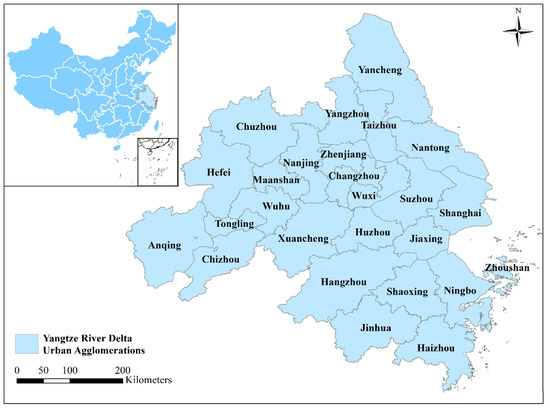
Figure 1.
The Yangtze River Delta urban agglomeration.
2.2. Data sources and Factors Introduction
2.2.1. Data Sources
The primary data sources include nighttime light data, statistical yearbooks and local bulletins, and administrative district vector data.
- (1)
- Nighttime light data. The nighttime light data source for this paper is cross-remote sensor-corrected NPP-VIIRS-like NTL data from 2000 to 2017 (Figure 2), with a spatial resolution of 500 m, a product period in years. It is accessible through the Harvard Dataverse platform (https://doi.org/10.7910/DVN/YGIVCD) (accessed on 29 May 2022). This dataset effectively improves the incomparability, over-saturation, and overflow of DMSP-OLS and NPP-VIIRS nighttime light data. It extends the time span over which nighttime light data is available and reflects the internal information of different cities [39]. In order to obtain the spatiotemporal distribution data of CO2 emission, we convert the annual nighttime light data into CO2 emission data by constructing an urban CO2 emission inversion model. After that, the CO2 emission raster data is resampled with a resampling resolution of 0.02° × 0.02°. The resampled data is converted to point data. By extracting the CO2 emission corresponding to each raster point, we finally obtained 30,334 CO2 emission points data per year;
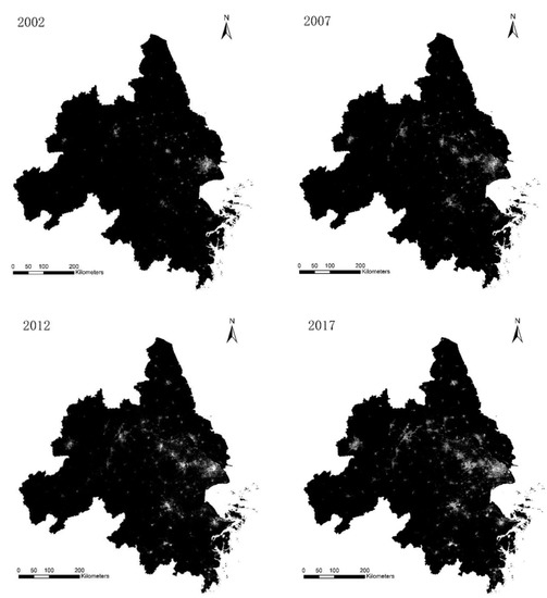 Figure 2. NPP-VIIRS-like nighttime light data.
- (2)
- Statistical yearbooks and local bulletins. All energy consumption and socioeconomic data come from (i) the statistical yearbooks and (ii) national economic and social development statistical bulletins. This data includes 26 cities in the YRD from 2000 to 2017 (http://www.stats.gov.cn/tjsj/ndsj/) (accessed on 29 May 2022);
- (3)
- Administrative division vector data. Due to the changes in administrative divisions in the YRD region during 2000–2017, some cities have been incorporated into or removed from the areas under their jurisdiction. Therefore, to eliminate the impact of administrative division changes on the inconsistency of statistical data standards, we select the administrative division vector data in 2020 as the standard (https://download.geofabrik.de/asia/china.html) (accessed on 29 May 2022).
2.2.2. Driving Factors
This study analyzes the impact of each indicator on CO2 emissions from the following four aspects: industrial structure, economic development level, urbanization and population, and infrastructure construction (Table 2). Here we provide a brief introduction of the selected driving factors.
Table 2.
Variable declaration.
Industrial structure: It refers to the linkages between industries and industrial composition. In the national economy, the industrial structure is divided into primary, secondary, and tertiary industries, while the degree of coordination of each industry affects the growth of CO2 emissions [40,41].
Economic development: The level of economic development includes gross regional product and foreign investment. The process of economic development can cause damage to the environment. The amount and the nature of foreign investment have a significant impact on local CO2 emissions, which may be positive or negative [42,43].
Urbanization and population: These factors mainly include urbanization rate and population density. Some studies have shown that the urbanization process contributes to the increase in CO2 emissions. However, this negative effect can be weakened through channels such as human capital accumulation and the promotion of cleaner production technologies [44].
Infrastructure construction: These factors mainly include construction area and road density. Studies have shown that expanding construction lands, such as a direct manifestation of industrialization and urbanization, contribute to the increase in CO2 emissions [45]. In addition, road density is one of the essential sources of CO2 emissions, and it can reflect the number of motor vehicles and tailpipe emissions.
2.3. Methods
The technical route of this study is shown in Figure 3. Firstly, data collection and preprocessing were carried out. Secondly, we used the IPCC method to calculate the carbon emission data of energy consumption in the study area from 2000 to 2017 by reviewing relevant literature. The inverse model was established to correct the carbon emission data at the municipal level by fitting the grayscale values of nighttime lights in the past years to obtain the final data for analysis. Next, we analyzed the data with two main contents. On the one hand, dynamic time wrapping and local spatial autocorrelation analysis were used to analyze the spatiotemporal characteristics of carbon emissions in the YRD region. On the other hand, the geographical detector model and the spatiotemporal geographical weighted regression model are used to investigate the influence of each influencing factor on the spatiotemporal distribution of carbon emissions. Finally, the results of the above analysis are combined to propose low-carbon development and carbon reduction policies that fit the current situation of carbon emissions in the YRD urban agglomeration.
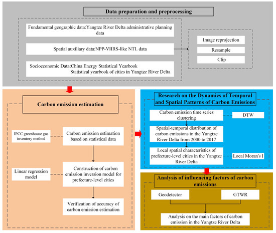
Figure 3.
Technology roadmap.
2.3.1. CO2 Emission Estimation
In this paper, we refer to the calculation method of Wang and others [46,47,48] and use the carbon emission factors of various energy sources determined by IPCC (2006) to derive the CO2 emissions of each city in the YRD. Then use the grayscale values of nighttime light data in the past years to conduct fitting analysis to explore their relationship.
In order to solve the problem of accuracy caused by downscaling to grid cells, this paper uses linear regression without intercept to construct a CO2 emission inversion model (Table 3). The results show an excellent fitting relationship between the grayscale values of nighttime light data and the statistical values of CO2 emissions, indicating that it is feasible to simulate CO2 emissions using nighttime light data.
Table 3.
Linear regression model of urban CO2 emission statistics and nighttime light gray value.
In order to test the reliability of the inversion model, the estimated values of the IPCC calculation method and the inverse CO2 emission values of each city in the YRD from 2000 to 2017 are correlated and analyzed. The fitting results are shown in Figure 4. The correlation coefficient (Pearson) is 0.967, indicating that it is feasible to use the inverse data to study the spatiotemporal distribution of CO2 emissions in the YRD region. However, it is found that the image does not pass through the origin, indicating that the inversion result is not entirely accurate, which is affected by the error of the regression function. In order to reduce the error, the adjustment factor is added to make the two results the same. The constructed inverse CO2 emission model and the adjustment factor are used to calculate the CO2 emissions of each city in the YRD. The calculation method is shown in Equations (1) and (2).
where is the year, is the adjustment factor for the year , is the CO2 emission value of the YRD calculated by IPCC calculation method in the year , is the CO2 emission value of the YRD calculated by the inversion model in the year , is the total grayscale value of night-time light in each city, is the fitting coefficient, is the CO2 emissions of each city calculated by the adjustment factor and the inversion model in the year .
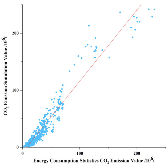
Figure 4.
Scatter plot of energy statistics CO2 emission values and fitted CO2 emission values.
2.3.2. Dynamic Time Wrapping and Hierarchical Clustering
Dynamic time wrapping (DTW) is a method used to calculate the similarity of time series [49,50,51]. Assuming that there are two time series data and with lengths m and n, respectively, the goal of the DTW algorithm is to find an optimal path such that the distance between the two time series is minimized. This path reflects the point-to-point correspondence between two time series, and the parameter represents the length of R. The distance between points and is expressed as , where . When calculating the optimal path, must satisfy the following conditions:
- Boundary condition: and ;
- Continuity: ,and ;
- Monotonicity: ,and .
The optimal path between and is shown in Equation (3).
The dynamic programming algorithm can solve the optimal path (see Equation (4)):
where .
The disadvantage of the DTW algorithm is that there is no threshold limit, and it aims only to find the best path, but the distance of this path may be very large or very small. Moreover, the algorithm cannot deal with outliers and outliers, and the suppression of noise is not processed. Therefore, it is necessary to detect outliers in the data before using this method. In this paper, the hierarchical clustering algorithm is no longer introduced. Readers can read references [52].
2.3.3. Local Spatial Autocorrelation Analysis
In this paper, we use the Anselin Local Moran’s I, which can identify spatial clusters with high and low values and can also identify outliers. Its calculation formula is shown in Equations (5) and (6).
where is the attribute of element , is the average value of the corresponding attribute, is the spatial weight between element and element , and where is the total number of elements as follows:
The calculation method of the score of statistical data is shown in Equations (7)–(9).
where:
When is positive, the attribute of the adjacent element is similar, and the elements can be clustered into one class. When the value is statistically significant at a 5% level (p < 0.05), the elements show high-high clustering or low-low clustering. When is negative, the adjacent elements contain different values, and the element is an outlier. When the value is statistically significant at a 5% level (p < 0.05), the elements show high-low abnormality or low-high abnormality. Otherwise, they are considered insignificant.
2.3.4. GDM and GTWR
This paper uses GDM (geographical detector model) with GTWR (geographical and temporal weighted regression) to explore the influence of each driver on the spatiotemporal distribution of carbon emissions.
GDM is a statistical method used to detect spatial heterogeneity and explain the driving forces behind it. This method is a powerful tool for driving force, factor analysis, and spatial analysis. It specializes in analyzing where the dependent variable Y is a type of numerical data and the independent variable X is a category of data. If Y and X are numerical values, then X can be converted into classified values by discretization. Therefore, the GDM can be used to predict a more reliable relationship between Y and X than classical regression, especially when the sample volume is less than 30. Based on these advantages, many scholars used GDM to detect the driving factors of CO2 emissions [53]. Based on these advantages, many scholars used GDM to detect the driving factors of CO2 emissions [54,55]. The core idea is that if the independent variable has an important influence on the dependent variable, then the spatial distribution of the independent variable and the dependent variable should be similar [56], and GDM does not need to consider multicollinearity between factors. The influence degree of the independent variable on the dependent variable is measured by q value. The expression of q is expressed as Equations (10) and (11) as follows:
where is the partition of the independent variable ; and are the number of units in partition and the whole region, respectively; and are the variances of the dependent variable for the partition and the entire region, respectively; are the sum of regional variance and total variance, respectively. The larger the value of , the greater the influence of the independent variable on the dependent variable . There are four types of geographical detectors, and the differentiation factor detector is mainly used in this paper.
Geographically weighted regression (GWR) is a standard model to study spatial heterogeneity, but GWR uses cross-sectional data. In empirical studies, to reduce local fluctuations in cross-sectional data, models are often constructed using the average of multiple years of data for the same indicator, which may result in some of the original information of the panel being lost. Although GWR adds geographical location to the regression coefficients and analyses the characteristics of the regression relationship with spatial location, it does not consider the actual problem’s temporal aspects. Geographically temporally weighted regression (GTWR) integrates temporal and spatial information into a weighting matrix to construct a spatiotemporal weighting matrix to explore the driver’s heterogeneity of factors in the temporal and spatial dimensions. The spatiotemporal weighting matrix is closer to reality than the spatial distance weighting matrix in the GWR model. In addition, the GTWR model can handle panel data, whereas GWR can only handle cross-sectional data. Thus, using the GTWR model to study the spatiotemporal heterogeneity of carbon emissions over long time series is more accurate. In recent years, more and more scholars have also adopted Spatiotemporal geo-weighted regression to study the spatiotemporal evolution of CO2 emissions of the drivers [57,58,59]. The expression of q is expressed as Equation (12) as follows:
where is the standard value of CO2 emissions for the ith city; is the spatiotemporal coordinate of the ith city; represents the constant term of the ith city point; is the regression coefficient of the kth explanatory variable of the ith city point; is the independent random error term, the mean is 0, and the variance is .
In addition, the choice of bandwidth has a more significant impact on the regression, so the cross-confirmation method is chosen as the spatiotemporal bandwidth in this paper.
3. Results and Discussion
3.1. CO2 Emission Time Series Clustering
In Figure 5, CO2 emissions have different time-varying characteristics. From 2000 to 2010, CO2 emissions in all cities showed an overall upward trend. From 2011 to 2012, the growth of CO2 emissions showed an “inflection point”, and the growth rate began to level off, even showing a decreasing trend in Shanghai, Shaoxing, Chizhou, Huzhou, and other cities. Overall, the growth of CO2 emissions in cities in the YRD firstly increased and then decreased, and some cities showed a negative growth trend around 2011.
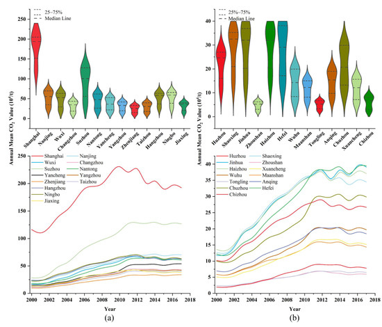
Figure 5.
Trend and distribution of CO2 emission in cities from 2000 to 2017. (a) Shanghai and other cities, (b) Huzhou and other cities.
The CO2 emissions of the cities in the YRD not only show differences in spatiotemporal dimensions but also have similarities. In order to quantify this degree of similarity and further explore the reasons that lead to the similar variation patterns exhibited by the cities in the YRD, this paper uses the DTW to analyze the time series data. Since we detected and processed the data for outliers in advance, there is no outlier, so the DTW algorithm can meet the needs of this paper. The similarity matrix between the CO2 emission time series of each city is calculated using DTW. The bottom-up hierarchical clustering algorithm is used to classify the city agglomerations into four classes based on the similarity matrix. The time-varying patterns are obtained based on the average CO2 emissions of each class of cities. The results are shown in Figure 6.
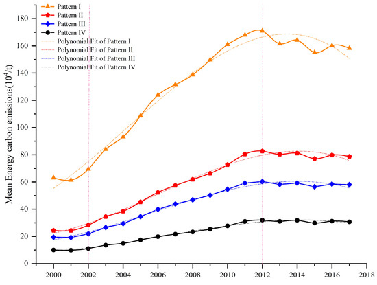
Figure 6.
CO2 emission time cluster.
Class I cities include Shanghai, Nanjing, Suzhou, Hefei, Wuxi, and Hangzhou. Those cities are the most densely industrialized, urbanized, densely populated, and economically developed regions in the YRD and therefore have the most significant impact on the energy carbon emissions in the YRD. There are three peaks in class I cities’ CO2 emission time series, respectively, in 2012, 2014, and 2017. After 2012, CO2 emissions experienced two significant fluctuations.
Class II cities include Shaoxing, Ningbo, Nantong, Changzhou, Wuhu, and Yancheng, which are mainly located along the coast with favorable climatic conditions, more developed tertiary industries, and smaller population sizes compared to class I cities. Class II cities’ CO2 emission capacity and potential are weaker than those of class I cities, but the overall CO2 emission capacity is stronger in the YRD region. The peak of the time series of CO2 emissions in class II cities occurred in 2012. After 2012, the CO2 fluctuation is not apparent and is in a stable transition stage.
Class III cities include Taizhou, Yangzhou, Haizhou, Zhenjiang, Huzhou, Maanshan, and Jiaxing, which are mainly located in central Jiangsu province and northern Zhejiang province. These cities have small population densities, underdeveloped secondary industries, low urbanization levels, and weak CO2 emission capacities. The change in CO2 emission time series of class III cities is similar to that of class II cities.
Class IV cities include Anqing, Jinhua, Zhoushan, Tongling, Chuzhou, Chizhou, and Xuancheng. These seven cities are mainly distributed in the central and southern parts of Anhui Province, with diverse landforms, a mild climate, developed primary industry, a small population density, a low level of secondary industry and urbanization, and weak CO2 emission capacity. The time series variation of CO2 emissions in class IV cities is small but reaches a peak in 2012.
It is worth noting that CO2 emissions in the time series of classes II, III, and IV cities show similar patterns of change, indicating that the three classes of cities are not only influenced by similar climate and policies but also jointly influenced by class I cities. Therefore, it is necessary to adopt synergistic management measures for such small and medium-sized cities.
3.2. Spatiotemporal Distribution of CO2 Emissions
The distribution of CO2 emissions in the YRD region in 2002, 2007, 2012, and 2017 is shown in Figure 7. The regions with high CO2 emissions are mainly concentrated in Class I cities. We can also notice that the CO2 emissions are high in some districts of Taizhou, Nantong, Ningbo, Yancheng, and Jinhua but low in other cities. From the long time series, the high CO2 emission area gradually expanded during 2002–2017, with Suzhou and Shanghai being the most significant.
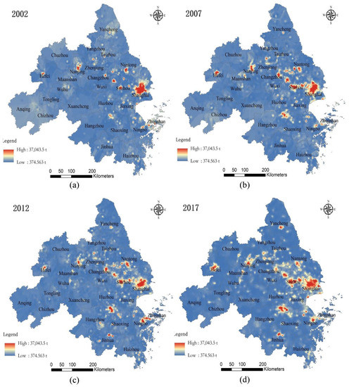
Figure 7.
Distribution of CO2 emissions.
The spatial correlation degree of CO2 emissions in the YRD urban agglomeration in 2002, 2007, 2012, and 2017 can be determined by local Moran’ I. The analysis results are shown in Figure 8. It can be seen that the degree of concentration of high CO2 emission aggregation areas in the YRD gradually increased during 2002–2017, mainly centering on class I cities. It is consistent with the spatiotemporal distribution of CO2 emissions in the YRD region, which shows that class I cities strongly influenced the spatiotemporal distribution of CO2 emissions in the YRD urban agglomeration. By comparing the local Moran’ I aggregation results in these four periods, it can be found that the high- and low-value aggregation ranges of cities of different classes vary greatly in different years. For class IV cities, the high aggregation areas of CO2 emissions in 2002 were mainly distributed in Anqing, Chizhou, Zhoushan, and northern Chuzhou. From 2002 to 2017, the high aggregation areas of CO2 emissions in class IV cities, except for Jinhua, decreased substantially, Anqing, Chizhou, and northern Chuzhou were transformed from high aggregation areas to low aggregation areas, and the high aggregation areas of Zhoushan kept converging to Ningbo. During this period, the high aggregation area of class I cities keeps getting larger, among which Wuxi, Suzhou, and Shanghai are the most significant. The high agglomeration areas in class II cities and class III cities have been expanding.
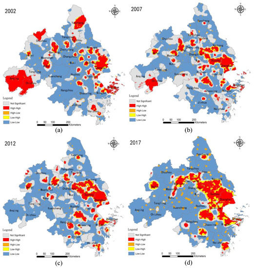
Figure 8.
Local Moran’ I.
This change is closely related to the characteristics of population mobility and related policies in different periods. With the acceleration of urbanization in the YRD, economic exchanges among cities are becoming closer and closer. Class I cities have greater development advantages than other cities, attracting a large number of immigrants. By analyzing the population flow data within the YRD in 2017, we found that the population migration of the YRD urban agglomeration has obvious city directionality, and class I and II cities are the primary aggregations of population flow in the YRD region at present. This trend is highly consistent with the local Moran’ I aggregation results. Before 2000, under reform and opening-up policies, the economy of the YRD developed rapidly, industries became increasingly intensive, and CO2 emissions increased. From 2002 to 2017, with the promotion of the regional coordinated development strategy, the core area of the YRD overflowed from the original Shanghai Pudong Development Zone, and labor and resource-intensive industries transferred to Suzhou, Wuxi, Jiaxing, Ningbo, and other peripheral areas. Therefore, the high CO2 emission agglomeration areas gradually spread around Shanghai, Suzhou, and other places.
3.3. Analysis of the Driving Factors of Energy Carbon Emissions in the YRD
At different stages of development, cities have different levels of economic growth, energy consumption, industrial structure, population, and policies. If we ignore these variations, we may draw biased or even misleading conclusions. Therefore, according to the peaks of CO2 emission concentrations in the four types of cities, we divided the whole study time series into the following three stages: Stage A (2000–2002), Stage B (2003–2012), and Stage C (2013–2017).
In order to explore the impact of each driving indicator on CO2 emissions, firstly, we calculated the values of each influencing factor from 2000 to 2017 using GDM, and the results are shown in Figure 9. Since GDM can only obtain the degree of influence when assessing each indicator and cannot explain the positivity and negativity of the driving factors, this paper further analyzes the magnitude of the influence of each indicator within each class of cities using the GTWR method. The results are shown in Figure 10.
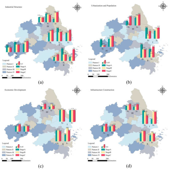
Figure 9.
Results of the GDM for each factor in the four types of cities.
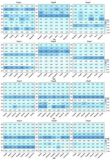
Figure 10.
Results of GTWR for each factor in the four types of cities. (a) Class I cities, (b) Class II cities, (c) Class III cities, (d) Class IV cities.
For the industrial structure, at all stages, X1 has played an inhibitory effect on the CO2 emissions in all cities. The impact on the CO2 emissions of I and II cities is gradually enhanced, and the impact on the CO2 emissions of III and IV cities is gradually weakened. Because class I and II cities developed earlier, after the initial completion of infrastructure, the government began to strengthen ecological control and optimize the environmental structure, leading to a gradual increase in the inhibitory effect on CO2 emissions. However, this inhibitory effect of cities in III and IV gradually weakens, which is mainly closely related to the acceleration of the industrialization process that drives the transformation of regional industrial structures from the first industry to the secondary and tertiary industries. X2 shows a downward trend in the four classes of cities, and X3 shows an upward trend. In Stage A, X2 is the main factor affecting the increase in CO2 emissions in four types of cities. In the early stages of city construction, X2 is the main driving force for economic development, increasing CO2 emissions. While in Stage B and Stage C, the influence of X2 on CO2 emissions gradually decreases because, with the proposal of the scientific outlook on development [60,61], higher requirements are put forward for the secondary industry to reduce overcapacity, and the tertiary industry, with lower energy consumption intensity, gradually plays a leading role in carbon emissions. Even in Stage C, the contribution of X3 to CO2 emissions in most cities exceeds that of X2. The impact of industrial structures on CO2 emissions in this paper is consistent with previous research results [40,41,62].
For the level of urbanization and population density, the contribution of X4 to CO2 emissions is gradually reduced for all four types of cities. It even plays a suppressive role at Stage C for I and II cities. The higher the level of urbanization, the stronger the regional innovation capability. This can better promote the application of new technologies and new energy sources, improve energy efficiency, and thus slow down the growth rate of carbon emissions. In contrast, the urbanization level of cities in III and IV is lower, and the first industry, as the primary source of carbon sinks in urbanization, is more developed than in other cities. With the proposed “red line for arable land” policy [63], the development of urban agriculture in III and IV cities has been emphasized, which gradually increases its inhibiting effect on CO2 emissions. The impact of X5 on CO2 emissions for all cities is always positive, with increasing population density bringing an increase in CO2 emissions [64,65]. In Stage A and Stage B, X5 has less influence on carbon emissions but has a greater impact in Stage C. This is mainly because as the per capita income of the population increases, people’s demand for unnecessary means of livelihood increases and consumer CO2 emissions increase. In addition, with the gradual deepening of the opening-up policy, the YRD attracts a large number of foreign investments with its unique location advantage, driving regional employment and talent migration. Compared with I and II cities, III and IV cities have the advantages of high development potential and low living pressure, attracting many people, thus driving the increase in carbon emissions.
For economic development, in I and II cities, the influence of X6 on CO2 emissions is first enhanced and then weakened. The impact on CO2 emissions of III and IV cities is gradually increasing. In Stage A and Stage B, the rapid economic development of I and II cities has led to the development of surrounding cities, making the CO2 emissions in the YRD gradually increase. On the other hand, since 2000, more than half of the country’s actual use of foreign investment has been invested in the YRD, while many polluting industries have been transferred to the YRD region, which makes the carbon emissions to increase significantly. The promoting effect of X7 on the CO2 emissions of the four types of cities has gradually increased. In Stage C, with the promotion of energy conservation and emission reduction policies, all kinds of cities have strengthened the supervision of the quality and nature of foreign investment under the background of “green“ and “low carbon“, making the influence of X7 on carbon emissions of various cities gradually weakened. However, energy consumption driven by economic development is still the primary source of CO2 emissions in I and II cities. Compared with I and II cities, the promoting effect of economic development level on CO2 emissions of III and IV cities has been weaker. The impact of economic development level on CO2 emissions conforms to the Environmental Kuznets curve (EKC) hypothesis [66,67]. In the late stage of urban development, the growth rate of CO2 emissions in the more developed regions gradually decreases.
For urban infrastructure construction, we can find that the impact of X8 on carbon emissions in class I cities is gradually weakening; it first increases and then decreases in class II cities; the effect of III and IV cities is growing progressively. It indirectly reflects that the development times of various cities are different. The development of I cities is earlier than class II, III, and IV cities. In Stage A of class I cities and Stage B of class II cities, urban construction is the main driving indicator of CO2 emission. The main reason is that cities at this stage actively develop infrastructure construction, which promotes the development of high energy-consuming industries such as steel and cement. In Stage C, the influence of X8 on CO2 emissions of class I and II cities gradually decreases, mainly because the construction of public infrastructure is completed, and the focus of urban spatial construction shifts to the construction of green areas in cities, which is developing towards a low-carbon direction. Compared with class I and II cities, the urbanization of class III and IV cities started later, and the influence of X8 on CO2 emissions is relatively lagging. Among I and II cities, the influence of X9 on CO2 emissions is enhanced first and then weakened. According to statistics, in Stage A and Stage B, the number of cars per 100 households jumped from 1.26 in 2000 to 8.04 in 2012, which further increased CO2 emissions. In Stage C, with the development of cities, the government vigorously develops the public transport system. It continuously promotes the development of the new energy automobile industry [68], resulting in decreased per capita transportation energy consumption and a significant decrease in CO2 emissions. For class III and IV cities, their road network construction starts later than in class I and II cities. The role of the public transportation system on road integration is not prominent, so the impact of X9 on CO2 emissions rose slowly, which is consistent with X8. On the other hand, X8 carries a variety of human activities such as industrial production, living and residence, transportation, etc. Therefore, the contribution of X9 to CO2 emissions is lower than X8 in all stages.
In addition, according to the results of GTWR, we can see the influence degree of some factors is heterogeneous within urban agglomerations. For example, from 2000 to 2017, the influence of X5 on the CO2 emissions of Nanjing and Hefei, class I cities, fluctuated greatly, and its influence first strengthened and then weakened, while the variations of other class I cities were moderate. Moreover, except in Haizhou, the influence of X2 on CO2 emissions in other class III cities increased first and then weakened. It reflects both similarities and differences in CO2 emissions among cities within the YRD urban agglomeration, so it is important to focus on the characteristics of each city when adopting synergistic management measures.
In the above discussion, we have analyzed the mechanism of carbon emissions from multiple perspectives, including time, space, city categories, and influencing factors. This paper has several limitations because of the complexity of the research problem. Firstly, due to the restriction of data acquisition, the data of indicators such as per capita consumption and solid waste disposal level were not included, which is a limitation for further analysis of the results; nevertheless, it is fortunate that the selected factors can reflect the development pattern of carbon emissions in the YRD urban agglomeration. Secondly, this paper is analyzed based on the prefecture-level cities in the YRD urban agglomeration. In the subsequent study, the adoption of county-level data for analysis can be considered to make the regional targeting of emission reduction measures more significant. In addition, we hope to form a complete system for analyzing a single element’s spatiotemporal characteristics and the divergent features of influencing factors in subsequent research. It will be of great significance if we can achieve the procedural and application of this methodological system. The scope of its application will not only be limited to the research of disciplinary fields. It will also have specific reference values for formulating various economic marketing programs.
4. Conclusions and Recommendations
4.1. Conclusions
This study takes the YRD urban agglomeration as the study area, analyzing and discussing its spatiotemporal divergences of CO2 emissions and influencing factors from 2000 to 2017. The main findings of the study are as follows:
- (1)
- From 2000 to 2017, the distribution of CO2 emissions in the YRD urban agglomerations showed an apparent spatial heterogeneity. Carbon emissions are consistently higher in Class I cities. From the perspective of long time series, the high CO2 emission value area has a tendency to expand gradually centered on itself, where this phenomenon is most significant in the class I cities;
- (2)
- The YRD region has a wide range of ‘high-high’ and ‘low-low’ regional aggregation and similarity in terms of spatial correlation. It has formed a high-emission agglomeration area with large cities such as Shanghai, Nanjing, and Suzhou as the core. Moreover, with the development over time, the “high-high” areas of CO2 emissions in the YRD urban agglomeration gradually converge around Wuxi, Suzhou, Shanghai, and other cities; meanwhile, the spatial distribution gradually decreases;
- (3)
- The influence of each driving indicator on CO2 emissions in urban agglomerations has both commonalities and differences. For Class I and II cities, the impact of urban construction on CO2 emissions is consistently high and stable in the early stage of urban development while significantly weakening in the later stage. For Class III and IV cities, the contribution of population density to CO2 emissions has always been at the top of the list and is gradually increasing. The primary industry has a suppressive effect on carbon emissions at all stages in all four cities, and this effect gradually increases in I and II cities and gradually decreases in class III and IV cities. At the same time, the urbanization rate has a suppressive effect on CO2 emissions at Stage C in all four types of cities. From the micro perspective, the degree of influence of individual factors is heterogeneous within urban agglomerations.
4.2. Policy Implications
In the process of urbanization, we should not only pursue speed but also focus on quality. We can not simply increase population quantity. In contrast, we need to reduce the growth of CO2 emissions brought on by the rise in population size through the human capital agglomeration effect. The development of emission reduction policies should focus on the characteristics of the city itself. According to the impact results of various factors in different cities, we put forward the following suggestions:
- (1)
- In more developed cities of Shanghai, Nanjing, and Hangzhou, the government should promote intensive land utilization to reduce carbon emissions;
- (2)
- In Shaoxing, Jiaxing, and other areas that are obviously radiated by Class I cities, the government should control new carbon source lands and explore potential carbon sink land to achieve regional carbon balance;
- (3)
- In the areas with good ecological resources and large-scale carbon sink lands, such as Anqing, Chizhou, and Xuancheng, the land use structure should be optimized to achieve high-quality development based on ensuring carbon sink function.
Author Contributions
Z.Z.: Conceptualization, Methodology, Data curation, Investigation, Writing—original draft, Software, Visualization, Project administration. J.Y.: Data curation, Investigation, Software, Writing—original draft. J.L.: Funding acquisition, Writing—review and editing, Supervision. H.Z.: Writing—review and editing. Q.W.: Writing—review and editing. Y.C.: Writing—review and editing. All authors have read and agreed to the published version of the manuscript.
Funding
This research was funded by the Assistance Program for Future Outstanding Talents of China University of Mining and Technology (Grant No. 2022WLJCRCZL002) and the National Natural Science Foundation of China (Grant No. 41872248) and the Priority Academic Program Development of Jiangsu Higher Education Institutions.
Institutional Review Board Statement
Not applicable.
Informed Consent Statement
Not applicable.
Data Availability Statement
The data that support the findings of this study are openly available at [https://zenodo.org/record/6769188#.YrrBR3ZBy3A], accessed on 10 May 2022.
Acknowledgments
We sincerely thank anonymous reviewers for helpful improvements to this manuscript.
Conflicts of Interest
The authors declare that they have no known competing financial interests or personal relationships that could have appeared to influence the work reported in this paper.
References
- World Meteorological Organization. Greenhouse Gas Concentrations in Atmosphere Reach yet Another High; World Meteorological Organization: Geneva, Switzerland, 2019; Available online: https://public.wmo.int/en/media/press-release/greenhouse-gas-concentrations-atmosphere-reach-yet-another-high (accessed on 10 May 2022).
- Parry, I.W.H.; Williams, R.C.; Goulder, L.H. When Can Carbon Abatement Policies Increase Welfare? The Fundamental Role of Distorted Factor Markets. J. Environ. Econ. Manag. 1999, 37, 52–84. [Google Scholar]
- World Meteorological Organization. Greenhouse Gas Concentrations Surge to New Record; World Meteorological Organization: Geneva, Switzerland, 2017; Available online: https://public.wmo.int/en/media/press-release/greenhouse-gas-concentrations-surge-new-record (accessed on 10 May 2022).
- Qing, G.; Luo, Y.; Huang, W.; Wang, W.; Yue, Z.; Wang, J.; Li, Q.; Jiang, S.; Sun, S. Driving Factors of Energy Consumption in the Developed Regions of Developing Countries: A Case of Zhejiang Province, China. Atmosphere 2021, 12, 1196. [Google Scholar] [CrossRef]
- Dhakal, S. Urban energy use and carbon emissions from cities in China and policy implications. Energy Policy 2009, 37, 4208–4219. [Google Scholar] [CrossRef]
- Cui, X.L.; Lei, Y.T.; Zhang, F.; Zhang, X.Y.; Wu, F. Mapping spatiotemporal variations of CO2 (carbon dioxide) emissions using nighttime light data in Guangdong Province. Phys. Chem. Earth 2019, 110, 89–98. [Google Scholar] [CrossRef]
- Zhao, Q. A Review of Pathways to Carbon Neutrality from Renewable Energy and Carbon Capture. In Proceedings of the 2021 5th International Conference on Advances in Energy, Environment and Chemical Science (AEECS 2021), Shanghai, China, 26–28 February 2021; Volume 245. [Google Scholar]
- Wang, C.; Chen, J.; Zou, J. Decomposition of energy-related CO2 emission in China: 1957–2000. Energy 2005, 30, 73–83. [Google Scholar] [CrossRef]
- He, Y.; Qin, C. Analysis of Provincial Carbon Emissions Based on Spatial Econometric Model. In Proceedings of the 2017 4th International Conference on Management Innovation and Business Innovation (ICMIBI 2017), Dubai, United Arab Emirates, 20–21 September 2017; Volume 81, pp. 105–110. [Google Scholar]
- Friedl, B.; Getzner, M. Determinants of CO2 emissions in a small open economy. Ecol. Econ. 2003, 45, 133–148. [Google Scholar] [CrossRef]
- Ang, B.W. The LMDI approach to decomposition analysis: A practical guide. Energy Policy 2005, 33, 867–871. [Google Scholar] [CrossRef]
- Al-mulali, U. Factors affecting CO2 emission in the Middle East: A panel data analysis. Energy 2012, 44, 564–569. [Google Scholar] [CrossRef]
- Wang, Z.; Yin, F.; Zhang, Y.; Zhang, X. An empirical research on the influencing factors of regional CO2 emissions: Evidence from Beijing city, China. Appl. Energy 2012, 100, 277–284. [Google Scholar] [CrossRef]
- Wang, S.; Fang, C.; Guan, X.; Pang, B.; Ma, H. Urbanisation, energy consumption, and carbon dioxide emissions in China: A panel data analysis of China’s provinces. Appl. Energy 2014, 136, 738–749. [Google Scholar] [CrossRef]
- Aye, G.C.; Edoja, P.E.; Charfeddine, L. Effect of economic growth on CO2 emission in developing countries: Evidence from a dynamic panel threshold model. Cogent Econ. Financ. 2017, 5, 1379239. [Google Scholar] [CrossRef]
- Ahmed, K.; Rehman, M.U.; Ozturk, I. What drives carbon dioxide emissions in the long-run? Evidence from selected South Asian Countries. Renew. Sustain. Energy Rev. 2017, 70, 1142–1153. [Google Scholar] [CrossRef]
- Tong, X.; Li, X.S.; Tong, L. Gray Correlative Empirical Research on Carbon Emissions and Influencing Factors in Hebei Province. In Proceedings of the 29th Chinese Control and Decision Conference (CCDC), Chongqing, China, 28–30 May 2017; pp. 3903–3908. [Google Scholar]
- Mohmmed, A.; Li, Z.; Olushola Arowolo, A.; Su, H.; Deng, X.; Najmuddin, O.; Zhang, Y. Driving factors of CO2 emissions and nexus with economic growth, development and human health in the Top Ten emitting countries. Resour. Conserv. Recycl. 2019, 148, 157–169. [Google Scholar] [CrossRef]
- Fan, Z.G.; Hu, Q. Research on influencing factors and countermeasures of industrial carbon emission in Hebei province based on Kaya model. In Proceedings of the 2nd International Conference on Air Pollution and Environmental Engineering (APEE), Xi’an, China, 15–16 December 2019. [Google Scholar]
- Liu, K.; Xue, M.Y.; Peng, M.J.; Wang, C.X. Impact of spatial structure of urban agglomeration on carbon emissions: An analysis of the Shandong Peninsula, China. Technol. Forecast. Soc. Chang. 2020, 161, 120313. [Google Scholar] [CrossRef]
- Wang, Y.X. The Spatial Distribution Characteristics of Carbon Emissions at County Level in the Harbin-Changchun Urban Agglomeration. Atmosphere 2021, 12, 1268. [Google Scholar] [CrossRef]
- Sha, W.; Chen, Y.; Wu, J.S.; Wang, Z.Y. Will polycentric cities cause more CO2 emissions? A case study of 232 Chinese cities. J. Environ. Sci. 2020, 96, 33–43. [Google Scholar] [CrossRef]
- Zhao, J.C.; Ji, G.X.; Yue, Y.L.; Lai, Z.Z.; Chen, Y.L.; Yang, D.Y.; Yang, X.; Wang, Z. Spatio-temporal dynamics of urban residential CO2 emissions and their driving forces in China using the integrated two nighttime light datasets. Appl. Energy 2019, 235, 612–624. [Google Scholar] [CrossRef]
- Li, R.; Sun, T. Research on Measurement of Regional Differences and Decomposition of Influencing Factors of Carbon Emissions of China’s Logistics Industry. Pol. J. Environ. Stud. 2021, 30, 3137–3150. [Google Scholar] [CrossRef]
- Zhao, Q.; Li, X.; Cui, X. Calculation of Carbon Dioxide Emission in Nanjing City and Its Influencing Factors. Mater. Sci. Processing Environ. Eng. Inf. Technol. 2014, 665, 517–520. [Google Scholar] [CrossRef]
- Piao, S.; Fang, J.; Ciais, P.; Peylin, P.; Huang, Y.; Sitch, S.; Wang, T. The carbon balance of terrestrial ecosystems in China. Nature 2009, 458, 1009-U82. [Google Scholar] [CrossRef]
- Chen, J.; Wang, H.; Zhang, X.; Chen, S.; Bao, Z. Analysis of carbon emissions from transportation in Beijing. Int. J. Serv. Technol. Manag. 2016, 22, 271–286. [Google Scholar] [CrossRef]
- Kenny, T.; Gray, N.F. Comparative performance of six carbon footprint models for use in Ireland. Environ. Impact Assess. Rev. 2009, 29, 1–6. [Google Scholar] [CrossRef]
- Zhu, E.; Deng, J.; Wang, H.; Wang, K.; Huang, L.; Zhu, G.; Belete, M.; Shahtahmassebi, A. Identify the optimization strategy of nitrogen fertilization level based on trade-off analysis between rice production and greenhouse gas emission. J. Clean. Prod. 2019, 239, 118060. [Google Scholar] [CrossRef]
- Han, R.; Li, L.; Zhang, X.; Lu, Z.; Zhu, S. Spatial-temporal Evolution Characteristics and Decoupling Analysis of Influencing Factors of China’s Aviation Carbon Emissions. Chin. Geogr. Sci. 2022, 32, 218–236. [Google Scholar] [CrossRef]
- Jiao, J.-L.; Qi, Y.-Y.; Cao, Q.; Liu, L.-C.; Liang, Q.-M. China’s targets for reducing the intensity of CO2 emissions by 2020. Energy Strategy Rev. 2013, 2, 176–181. [Google Scholar] [CrossRef]
- Shu, Y.; Lam, N.S.N. Spatial disaggregation of carbon dioxide emissions from road traffic based on multiple linear regression model. Atmos. Environ. 2011, 45, 634–640. [Google Scholar] [CrossRef]
- Zhou, Y.; Zhang, J.; Hu, S. Regression analysis and driving force model building of CO2 emissions in China. Sci. Rep. 2021, 11, 6715. [Google Scholar] [CrossRef]
- Liu, Y.; Xiao, H.; Zhang, N. Industrial Carbon Emissions of China’s Regions: A Spatial Econometric Analysis. Sustainability 2016, 8, 210. [Google Scholar] [CrossRef]
- Videras, J. Exploring spatial patterns of carbon emissions in the USA: A geographically weighted regression approach. Popul. Environ. 2014, 36, 137–154. [Google Scholar] [CrossRef]
- Tong, X.; Chen, K.; Li, X. Spatial Low Carbon Econometric Development of China Provincials in the view of International Trade. In Proceedings of the 2015 27th Chinese Control and Decision Conference (CCDC), Qingdao, China, 23–25 May 2015; pp. 3826–3831. [Google Scholar]
- Xia, X. FDI, Economic Growth and China’s Carbon Emission Intensity: An Empirical Study Based on Spatial Panel Econometric Model. In Proceedings of the 4th International Conference on Advances in Energy Resources and Environment Engineering, Shanghai, China, 16–18 August 2019; Volume 237. [Google Scholar]
- Wang, S.J.; Shi, C.Y.; Fang, C.L.; Feng, K.S. Examining the spatial variations of determinants of energy-related CO2 emissions in China at the city level using Geographically Weighted Regression Model. Appl. Energy 2019, 235, 95–105. [Google Scholar] [CrossRef]
- Chen, Z.; Yu, B.; Yang, C.; Zhou, Y.; Yao, S.; Qian, X.; Wang, C.; Wu, B.; Wu, J. An extended time series (2000–2018) of global NPP-VIIRS-like nighttime light data from a cross-sensor calibration. Earth Syst. Sci. Data 2021, 13, 889–906. [Google Scholar] [CrossRef]
- Lin, B.; Chen, Y. Will land transport infrastructure affect the energy and carbon dioxide emissions performance of China’s manufacturing industry? Appl. Energy 2020, 260, 114266. [Google Scholar] [CrossRef]
- Qi, J. Study on the threshold effect of China’s industrial structure on carbon emission. In Proceedings of the 2020 6th International Conference on Advances in Energy, Environment and Chemical Engineering, Zhongqing, China, 20–22 November 2020; Volume 546. [Google Scholar]
- Ma, X.; Wang, C.; Dong, B.; Gu, G.; Chen, R.; Li, Y.; Zou, H.; Zhang, W.; Li, Q. Carbon emissions from energy consumption in China: Its measurement and driving factors. Sci. Total Environ. 2019, 648, 1411–1420. [Google Scholar] [CrossRef]
- Zhang, W.; Li, G.; Uddin, M.K.; Guo, S. Environmental regulation, Foreign investment behavior, and carbon emissions for 30 provinces in China. J. Clean. Prod. 2020, 248, 119208. [Google Scholar] [CrossRef]
- Yao, X.; Kou, D.; Shao, S.; Li, X.; Wang, W.; Zhang, C. Can urbanization process and carbon emission abatement be harmonious? New evidence from China. Environ. Impact Assess. Rev. 2018, 71, 70–83. [Google Scholar] [CrossRef]
- Du, Q.; Lu, X.; Li, Y.; Wu, M.; Bai, L.; Yu, M. Carbon Emissions in China’s Construction Industry: Calculations, Factors and Regions. Int. J. Environ. Res. Public Health 2018, 15, 1220. [Google Scholar] [CrossRef]
- Jin, X.; Luo, L.; Chen, X. City Carbon Dioxide Emission Calculation for Low Carbon Development Strategies. In Proceedings of the International Conference on Frontiers of Environment, Energy and Bioscience (ICFEEB 2013), Beijing, China, 24–25 October 2013; pp. 835–840. [Google Scholar]
- Lee, J.; Kang, S.; Kim, S.; Kim, K.-H.; Jeon, E.-C. Development of municipal solid waste classification in Korea based on fossil carbon fraction. J. Air Waste Manag. Assoc. 2015, 65, 1256–1260. [Google Scholar] [CrossRef]
- Wang, Y.; Niu, Y.; Li, M.; Yu, Q.; Chen, W. Spatial structure and carbon emission of urban agglomerations: Spatiotemporal characteristics and driving forces. Sustain. Cities Soc. 2022, 78, 103600. [Google Scholar] [CrossRef]
- Chen, Y.; Liu, X.; Li, X.; Liu, X.; Yao, Y.; Hu, G.; Xu, X.; Pei, F. Delineating urban functional areas with building-level social media data: A dynamic time warping (DTW) distance based k-medoids method. Landsc. Urban Plan. 2017, 160, 48–60. [Google Scholar] [CrossRef]
- Ramaker, H.J.; van Sprang, E.N.M.; Westerhuis, J.A.; Boelens, H.F.M.; Smilde, A.K. Dynamic time warping of spectroscopic BATCH data. Anal. Chim. Acta 2003, 498, 133–153. [Google Scholar] [CrossRef]
- Wu, Q.; Guo, R.; Luo, J.; Chen, C. Spatiotemporal evolution and the driving factors of PM2.5 in Chinese urban agglomerations between 2000 and 2017. Ecol. Indic. 2021, 125, 107491. [Google Scholar]
- Murtagh, F. A Survey of Recent Advances in Hierarchical Clustering Algorithms. Comput. J. 1983, 26, 354–359. [Google Scholar] [CrossRef]
- Wang, J.F.; Xu, C.D. Geodetector: Principle and prospective. Acta Geogr. Sin. 2017, 72, 116–134. [Google Scholar]
- Fang, Y.; Wang, L.; Ren, Z.; Yang, Y.; Mou, C.; Qu, Q. Spatial Heterogeneity of Energy-Related CO2 Emission Growth Rates around the World and Their Determinants during 1990–2014. Energies 2017, 10, 367. [Google Scholar] [CrossRef]
- Yang, Y.; Wang, L.; Cao, Z.; Mou, C.; Shen, L.; Zhao, J.; Fang, Y. CO2 emissions from cement industry in China: A bottom-up estimation from factory to regional and national levels. J. Geogr. Sci. 2017, 27, 711–730. [Google Scholar] [CrossRef]
- Wang, J.-F.; Li, X.-H.; Christakos, G.; Liao, Y.-L.; Zhang, T.; Gu, X.; Zheng, X.-Y. Geographical Detectors-Based Health Risk Assessment and its Application in the Neural Tube Defects Study of the Heshun Region, China. Int. J. Geogr. Inf. Sci. 2010, 24, 107–127. [Google Scholar] [CrossRef]
- Dong, F.; Li, J.; Wang, Y.; Zhang, X.; Zhang, S.; Zhang, S. Drivers of the decoupling indicator between the economic growth and energy-related CO2 in China: A revisit from the perspectives of decomposition and spatiotemporal heterogeneity. Sci. Total Environ. 2019, 685, 631–658. [Google Scholar] [CrossRef]
- Li, W.; Ji, Z.; Dong, F. Spatio-temporal evolution relationships between provincial CO2 emissions and driving factors using geographically and temporally weighted regression model. Sustain. Cities Soc. 2022, 81, 103836. [Google Scholar] [CrossRef]
- Dong, F.; Li, J.; Zhang, S.; Wang, Y.; Sun, Z. Sensitivity analysis and spatial-temporal heterogeneity of CO2 emission intensity: Evidence from China. Resour. Conserv. Recycl. 2019, 150, 104398. [Google Scholar] [CrossRef]
- Environmental Protection Administration. Green GDP Provides a Scientific Basis for Cadres’ Performance Assessment. Available online: http://www.gov.cn/jrzg/2006-09/08/content_382794.htm (accessed on 29 May 2022).
- Zhang, L.; Li, L. Scientific Development View is the Inheritance and Innovation of Marxist Development Theory. Guangming Daily. 23 July 2006. Available online: https://www.gmw.cn/01gmrb/2006-07/23/content_453777.htm (accessed on 10 May 2022).
- Chunmei, L.; Maosheng, D.; Xiliang, Z.; Jieting, Z.; Lingling, Z.; Guangping, H. Empirical Research on the Contributions of Industrial Restructuring to Low-Carbon Development. Energy Procedia 2011, 5, 834–838. [Google Scholar] [CrossRef][Green Version]
- Ministry of Land and Resources of the People’s Republic of China. Development of Red Line Project—Action Plan 2010; Ministry of Land and Resources of the People’s Republic of China: Beijing, China, 2010. Available online: http://www.gov.cn/gzdt/2010-04/14/content_1580477.htm (accessed on 10 May 2022).
- Han, X.; Cao, T.; Sun, T. Analysis on the variation rule and influencing factors of energy consumption carbon emission intensity in China’s urbanization construction. J. Clean. Prod. 2019, 238, 117958. [Google Scholar] [CrossRef]
- Liu, J.; Li, M.; Ding, Y. Econometric analysis of the impact of the urban population size on carbon dioxide (CO2) emissions in China. Environ. Dev. Sustain. 2021, 23, 18186–18203. [Google Scholar] [CrossRef]
- Azizalrahman, H.; Hasyimi, V. A model for urban sector drivers of carbon emissions. Sustain. Cities Soc. 2019, 44, 46–55. [Google Scholar] [CrossRef]
- Lyu, W.; Li, Y.; Guan, D.; Zhao, H.; Zhang, Q.; Liu, Z. Driving forces of Chinese primary air pollution emissions: An index decomposition analysis. J. Clean. Prod. 2016, 133, 136–144. [Google Scholar] [CrossRef]
- State Council of the People’s Republic of China. Energy-Saving and New Energy Vehicle Industry Development Plan (2012–2020); State Council of the People’s Republic of China: Beijing, China, 2012. Available online: http://www.gov.cn/zwgk/2012-07/09/content_2179032.htm (accessed on 10 May 2022).
Publisher’s Note: MDPI stays neutral with regard to jurisdictional claims in published maps and institutional affiliations. |
© 2022 by the authors. Licensee MDPI, Basel, Switzerland. This article is an open access article distributed under the terms and conditions of the Creative Commons Attribution (CC BY) license (https://creativecommons.org/licenses/by/4.0/).