Article

A Social Vulnerability Index for Air Pollution and Its Spatially Varying Relationship to PM2.5 in Uganda

1
Department of Environmental Global Health, University of Florida, Gainesville, FL 32610, USA
2
Department of Geography, University of Florida, Gainesville, FL 32611, USA
3
Department of Computer Science, Makerere University, Kampala P.O. Box 7062, Uganda
*
Author to whom correspondence should be addressed.
Atmosphere 2022, 13(8), 1169; https://doi.org/10.3390/atmos13081169
Submission received: 14 June 2022 / Revised: 16 July 2022 / Accepted: 21 July 2022 / Published: 23 July 2022
(This article belongs to the Special Issue Ambient and Indoor Air Pollution Status in Africa)

Abstract

:
Fine particulate matter (PM2.5) is a ubiquitous air pollutant that is harmful to human health. Social vulnerability indices (SVIs) are calculated to determine where vulnerable populations are located. We developed an SVI for Uganda to identify areas with high vulnerability and exposure to air pollution. The 2014 national census was used to create the SVI. Mean PM2.5 at the subcounty level was estimated using global PM2.5 estimates. The mean PM2.5 for Kampala at the parish level was estimated using low-cost PM2.5 sensors and spatial interpolation. A local indicator of spatial association (LISA) was performed to determine significant spatial clusters of social vulnerability, and a bivariate analysis was performed to identify where significant associations were between SVI and annual PM2.5 mean concentrations. The LISA results showed significant clustering of high SVI in the northern and western regions of the country. The spatial bivariate analysis showed positive linear associations between SVI and PM2.5 concentration in subcounties in the northern, western, and central regions of Uganda, as well as in certain northern parishes in Kampala. Our approach identified areas facing both high social vulnerability and air pollution levels. These areas can be prioritized for health interventions and policy to reduce the impact of ambient PM2.5.

1. Introduction

Current estimates suggest that exposure of populations in Africa to outdoor air pollution causes approximately 780,000 deaths annually [1], accounting for more deaths than HIV/AIDS in Africa [2,3]. The latest global burden of disease (GBD) estimates for sub-Saharan Africa (SSA) indicate that air pollution caused 4513.83 disability-adjusted life years (DALYs) per 100,000 people in 2019, ranking second overall in terms of DALYs for the SSA region [4]. Additionally, the annual fine particulate matter (PM2.5) air pollution concentration in SSA (47 µg/m3 in 2017) far exceeds the World Health Organization (WHO) standard of 5 µg/m3.
Acute and chronic exposure to elevated levels of PM2.5 is especially harmful to vulnerable populations that include children, the elderly, and those of lower socioeconomic status (SES) [5]. However, for most lower- and middle-income countries (LMICs) of SSA, little is known regarding which geographic areas may be most vulnerable to health impacts from air pollution. Consequently, any interventions may leave out the most vulnerable, further increasing their risk to the effects of air pollution.
Vulnerability is broadly considered a contextual term. In certain contexts, vulnerability defines populations and individuals who are at greater risk of having poor health outcomes related to disease [6]. In other contexts, vulnerability can describe how much an individual or population is affected by various environmental hazards [7]. There are two main types of vulnerability, social vulnerability and biophysical vulnerability. Social vulnerability considers a population’s social or demographic characteristics, such as age, gender, ethnicity, disability, geographic location (e.g., rurality), infrastructure deficits, housing, and financial viability [7]. Alternatively, biophysical vulnerability refers to the likely occurrence of any given environmental hazard (e.g., air pollution) [8].
Social vulnerability is conceptualized as regional sensitivity to PM2.5 and the capacity to cope with its effects [9]. Sensitivity refers to how much an area is affected by exposure to various environmental hazards, as determined by the area’s demographic distribution and social structure [9]. The social structural factors that are most important to understanding impacts of environmental pollution include educational level, income status, and social trust or belief in other members of their society [10]. An environmental justice lens posits that social inequality, and the unequal distribution of social resources contribute to disparities in exposure to environmental pollutants, such as ambient PM2.5 [9]. Capacity to cope refers to whether a region can accommodate the impacts of PM2.5 pollution, which is dependent on the economic (support to solve and improve air pollution), ecological (absorption of human waste and pollution), and social capacities (hazard mitigation actions) of the area [9].
Spatially mapping PM2.5 and social vulnerability to describe a bivariate relationship is also important to identify areas that have both high social vulnerability and high PM2.5 exposure. Social vulnerability indices have been analyzed in other hazard contexts, such as landslides, earthquakes, infectious diseases, windstorms, and floods [11,12,13,14]. Air pollution hazards have been less explored, particularly in SSA. It is important to investigate geographic overlaps of social vulnerability and air pollution hazards because of the implications for chronic and long-term health effects in vulnerable communities.
This paper focuses on evaluating combined social and biophysical vulnerability to air pollution. More specifically, we investigate fine particulate matter (PM2.5) air pollution in the East African country of Uganda and its capital city, Kampala. This African country was chosen as it has high variability in both social vulnerability and PM2.5 exposure. This study is the first of its kind to consider social vulnerability in the context of ambient air pollution in SSA. We created an air-pollution-specific social vulnerability index (SVI) for Uganda and determined the spatially varying relationship between PM2.5 exposure and social vulnerability. The questions that this paper will address are: (1) What is the social vulnerability profile of Uganda by subcounty? (2) Is there any significant local clustering of high or low vulnerability across subcounties? (3) What is the nationwide scale association between spatial estimates of ambient PM2.5 and SVI in subcounties in Uganda? (4) What is the local-scale association between more spatially refined estimates of PM2.5 and SVI in parishes in Kampala, Uganda? (5) Where are the areas of particular concern in Uganda with high SVI and high PM2.5 mean concentrations?

2. Materials and Methods

2.1. Study Area

In this study, we performed a national-scale analysis of Uganda and a city-scale analysis of Uganda’s capital city of Kampala. Uganda is a landlocked country in East Africa, with an area of 241,038 km2 [15]. Uganda is surrounded by South Sudan to the north, Tanzania and Rwanda to the south, Kenya to the east, and the Democratic Republic of Congo to the west [16]. Classified as a low-income country by the World Bank, agriculture remains the primary economic driver in Uganda. Faced with a high fertility rate and high under-five child mortality rate, Uganda also has one of the highest population growth rates in the world at 3% [17]. While the rural area remains home to most Ugandans (about 84% of the total population), the urban growth rate is rapidly increasing, and slums have become a significant feature of Uganda’s urban landscape [13]. Kampala is a rapidly expanding urban city as it hosts almost 40% of Uganda’s urban population and is the economic center of the country [18].
In Uganda, ambient PM2.5 sources derive from the country’s rapid urbanization, industrialization, increasing motor vehicle ownership, and burning biomass for domestic energy use [19]. In a recent study, Uganda’s 2020 annual PM2.5 average concentration was 52.22 µg/m3, far exceeding the WHO PM2.5 standard of 5 µg/m3 annual and 15 µg/m3 daily mean concentration [20,21]. This confluence of factors makes it imperative to describe and visualize the social vulnerability landscape of the country by subcounty with a further focus on the Kampala district by parish.

2.2. Description of Study Data

2.2.1. Uganda Bureau of Statistics Census 2014

This study utilized Uganda’s 2014 national census data, which is the most recent available population data for the country [22]. We analyzed data for nationwide and localized (District of Kampala) analyses for the subcounty and parish levels, respectively. Subcounty data were used at the national level because it was granular enough to highlight the heterogenous nature of the data and at a large-enough scale to show a representative portion of the country. The data were for 1436 (94%) of Uganda’s 1520 subcounties. Parishes were chosen at the localized level because they were the smallest scale at which the data were available. There were 94 parishes in the Kampala district available from the 2014 national census, but 99 in the shapefile, indicating 95% coverage. Subcounties and parishes were excluded from the analysis if they did not match the publicly available census and GIS data [23].

2.2.2. Criteria for Selection of Census Variables

Census variables were selected (see descriptions in Table 1) that comprehensively relate to population and household composition, education and literacy, birth registration, parental survival, work status, housing conditions, health and hygiene, and community services, among other categories. These variables are consistent with previous research on exposure and social vulnerability to air pollution [9,24,25]. We selected other variables based on contextual knowledge of what is considered essential for characterizing social vulnerability and air pollution exposure in Uganda [26,27,28] and further condensed them using a correlation matrix to determine the similarity among variables. From the results of the correlation matrix, those variables that had a score of 0.7 or higher were paired, and one variable was chosen based on how much variance was noted across subcounties (higher variance was chosen), resulting in 21 census variables for further analysis. Each of the 21 variables was normalized appropriately and used at the subcounty and parish levels.
Following a hierarchical index construction method [29], the 21 variables were then grouped into seven themes, including age dependency, social, air quality, communication, economy, health, and housing (Table 1). An age dependency theme was included because children and elderly individuals are known to be dependent physically, financially, and socially on other members outside of their age group [30]. A communication theme was selected because it is crucial in the case of communicating risk and recommended protective behaviors during high air pollution events. Households without communication devices will not be able to respond to any public health advisory to mitigate exposure, and illiterate adults are less likely to be aware of the dangers of air pollution on health. The economy theme is related to a person’s income potential, housing situation, and capacity to adapt to environmental hazards [30]. The two variables representing the economic theme are households where no member possesses a bank account and households dependent on subsistence farming. Since these variables are highly correlated, we regressed one on the other, and the residual of the bank account values was used in calculating the overall score. The health theme addresses access to health facilities and water, sanitation, and hygiene (WaSH). Access to health facilities can influence how populations respond to adverse health effects caused by air pollution. A lack of WaSH has overlapping health risks with air pollution. For example, a lack of WaSH can make people more susceptible to respiratory infections, and severity of respiratory infections is related to air pollution exposure [31]. The social theme addresses individuals in the population, such as those with disabilities, orphaned, or widowed, who face compounding social vulnerabilities that make them less able to protect themselves from air pollution exposure. The housing theme includes temporary housing units and renter-occupied housing. Temporary housing units are more likely to be poorly constructed, using temporary materials for the roofing, walls, and flooring (e.g., tin or iron sheets). Additionally, temporary and renter-occupied homes are often less well maintained than permanent or owner-occupied housing [32]. Poorly constructed dwelling units can impact the ventilation and airflow throughout the house and allow more ambient air pollution to enter. The air quality theme was included because of the need to consider sources of household air pollution that can add to air pollution exposure and thus cause more significant health effects from poor air quality.

2.2.3. Nationwide Estimates of PM2.5

Gridded data of annual average PM2.5 concentration at the surface layer for 2014 were obtained from the Atmospheric Composition Analysis Group’s (ACAG) global PM2.5 estimates [33], which are at a spatial resolution of 0.1° × 0.1° (1 km × 1 km grid) [34]. The ACAG used combined aerosol optical depth (AOD) data from the satellite-borne instruments MODIS (Moderate Resolution Imaging Spectroradiometer, Raytheon Santa Barbara Remote Sensing (SBRS), Goleta, CA, USA), MISR (Multiangle Imaging Spectroradiometer, NASA/Jet Propulsion Laboratory (JPL), La Cañada Flintridge in California, CA, USA), and SeaWiFS (Hughes Santa Barbara Research Center (SBRC), Santa Barbara, USA) satellite [34]. Satellite observations were then calibrated to global ground-based observations of PM2.5 using data from the World Health Organization (WHO) with geographically weighted regression (GWR) [35].

2.2.4. Ground-Level PM2.5 Monitoring Data for the Kampala Metropolitan Area

Annual (2020) PM2.5 concentrations from ground monitoring data for the Greater Kampala Metropolitan Area (GKMA) and its surroundings were provided by the AirQo project in Kampala, UG. AirQo’s monitoring network is composed of low-cost sensors that measure PM2.5 in near real time. Details about the sensor network are published elsewhere [21,36]. Briefly, the ground monitoring data used in this analysis come from 21 air monitoring sites with measurements spanning 1 January 2020 to 31 December 2020 [21]. The PM2.5 concentrations were averaged for the entire year of 2020 for use in this analysis, matching the average period used in the ACAG dataset. It is not necessary to use other measures of central tendency because the AirQo data distribution approximates a normal distribution.

2.3. Data Analysis Processes

2.3.1. Creating the Social Vulnerability Index

We constructed the social vulnerability index (SVI) following the United States Centers for Disease Control and Prevention (CDC) hierarchical methodology, where each of the 21 census variables (from Section 2.2.2) was ranked from highest to lowest across all subcounties in Uganda (N = 1436) [30]. We calculated each subcounty’s percentile rank to census each variable [30]. For instance, the percentage of households that live in temporary dwelling units by subcounty was ranked from highest to lowest. Each rank was divided by the number of subcounties (N), which were both subtracted by 1 to scale values between 0 and 1, and then the percentile rank was achieved (see example in Document S1 of Supplementary Materials). We then calculated a percentile rank for each of the seven themes based on a sum of percentile ranks of the variables within that theme [30]. Finally, we calculated an overall percentile rank as the sum of the theme percentile rankings [30]. A percentile rank indicates the proportion of scores in a distribution that a specific score is greater than or equal to using the following formula:
P e r c e n t i l e   R a n k = ( R a n k 1 ) ( N 1 )
where N is the total number of data points, and all sequences of ties are assigned the smallest of the corresponding ranks [30]. The lowest possible score is 0 (low social vulnerability), and the highest possible score is 1; meaning the district has the highest social vulnerability index value. We calculated the SVI values in Microsoft Excel for each subcounty in UG and each parish in Kampala. SVI scores were imported to ArcGIS and joined to subcounty and parish boundary shapefiles using a field of unique identifiers for each geographic unit.

2.3.2. Estimating Annual PM2.5 at the Subcounty Level

Sub-county-level PM2.5 calculations were estimated using the ACAG PM2.5 surface layer estimates for 2014. For each subcounty administrative boundary, we calculated the mean PM2.5 using the Zonal Statistics tool in ArcGIS (version 2.9.2, ESRI, Redlands, CA, USA). This tool summarizes the values of the global PM2.5 raster within the zones of another dataset, in this case, the country of Uganda, and reports the results as a table [37].

2.3.3. Estimating Annual PM2.5 within Kampala at the Parish Level Using Spatial Interpolation

The Geostatistical Analyst tool in ArcGIS was used to create a PM2.5 raster of the area using inverse distance weighting (IDW) and data from the 21 PM2.5 ground monitors that were in and around the Kampala district. We applied the default IDW parameters in ArcGIS. The Ordinary Kriging (OK) tool in ArcGIS was also used to create an alternate PM2.5 raster surface of the Kampala area, using the same 21 monitors located within and surrounding the Kampala district. Again, default parameters for OK were applied to estimate the PM2.5 at the surface layer. The Zonal Statistics tool in ArcGIS was used for the IDW- and OK-derived PM2.5 values to calculate parish-level PM2.5 mean values for Kampala.

2.3.4. Determining SVI Clustering among Subcounties

We performed Global Moran’s I test to determine spatial clustering or dispersion among the SVI scores in Uganda. We used the incremental spatial autocorrelation tool to determine the optimum distance threshold/band based on the z-score. This tool indicated that 148 km is the optimum distance corresponding to the most significant levels of positive spatial autocorrelation. We also performed a local indicator of spatial association (LISA) to determine the location of statistically significant SVI spatial clusters.

2.3.5. Determining Local Association between PM2.5 and SVI Score

We used the local bivariate relationship tool to identify significant localized associations between SVI and annual PM2.5 mean concentrations. For the nationwide sub-county-level analysis, we set the number of neighbors at 430. For the Kampala parish-level analysis, we set the number of neighbors at 30. Distances for geographic coordinates were analyzed using chordal distance in meters. We set the number of permutations at 199 and the confidence level at the default of 90% for the sub-county- and parish-level analyses. These parameters are standard, and results will be robust enough to detect strong and relatively weak relationships [38].

3. Results

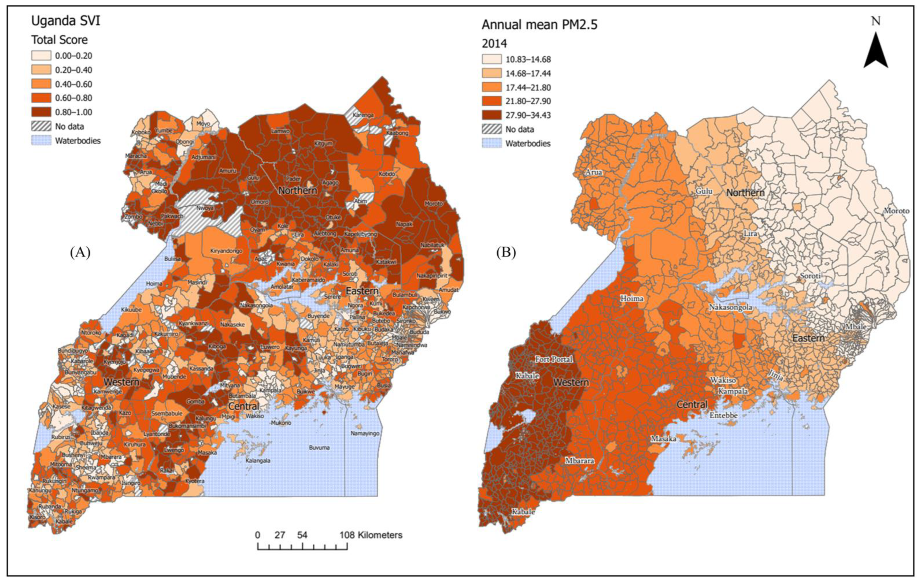
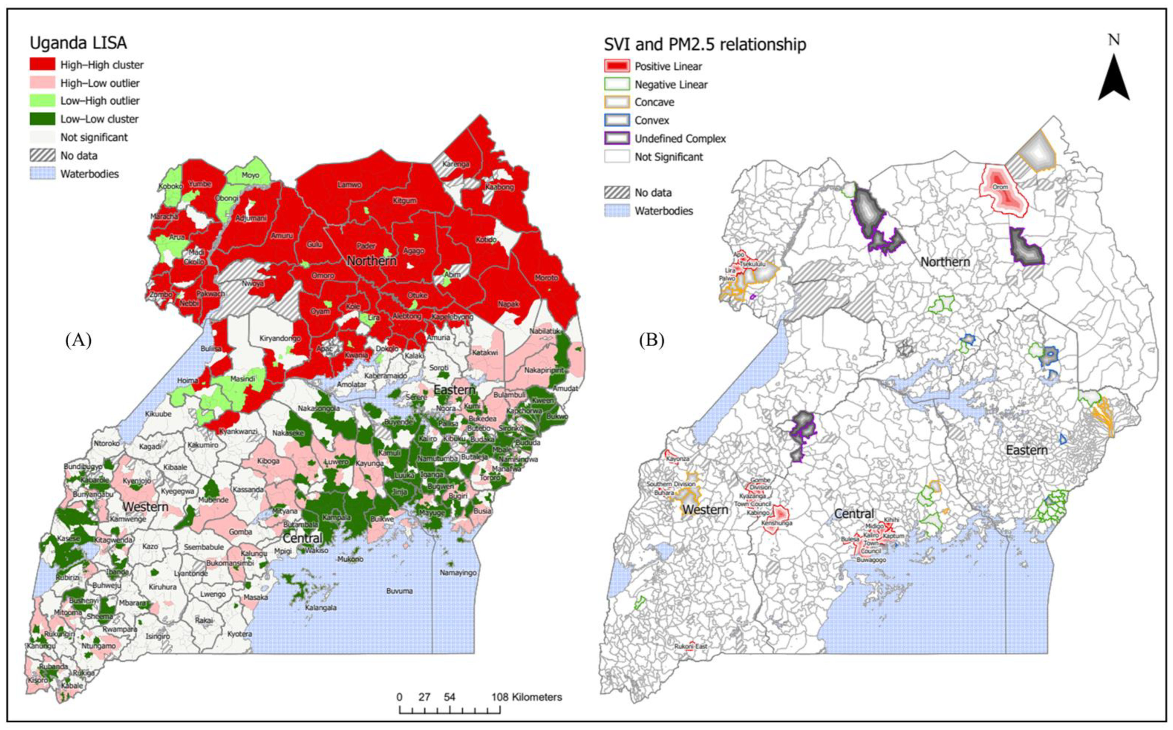
3.1. Nationwide Analysis

Mapping of the sub-county-level social vulnerability index (SVI) showed a clear spatial pattern across Uganda, with several subcounties exhibiting spatial clusters of very high social vulnerability to air pollution and other subcounties exhibiting clusters of low social vulnerability to air pollution. Figure 1A shows that UG’s subcounties in the highest quintile (0.8 to 1) predominate in the north. In contrast, the subcounties with SVI scores in the lowest quintile (0 to 0.2) were mainly in the south. The annual mean PM2.5 concentrations for the year 2014 per subcounty as estimated by the ACAG dataset are shown in Figure 1B. The figure shows a spatial gradation of low (10.83 μ g/m3) to high (34.43 μ g/m3) PM2.5 concentration, with the levels increasing from the northeast to the southwest, respectively.
Global Moran’s I test for SVI resulted in a value of 0.146, with a p-value < 0.001 (Figure S1 of Supplementary Materials). This result indicates a significant positive spatial autocorrelation and, thus, spatial clustering of SVI. Figure 2A shows statistically significant spatial clusters of high vulnerability for subcounties surrounded by other high-vulnerability subcounties (shown in red), occurring mainly in the country’s northern region. The low-vulnerability areas surrounded by other low-vulnerability areas (shown in green) occur primarily in the country’s southwestern and southeastern areas. The pink-colored districts have high vulnerability scores but are surrounded by low-vulnerability districts and occur primarily in the southeastern and central parts of the country. The light-green subcounties are subcounties with low vulnerability scores but surrounded by areas with high vulnerability scores; these districts are in the country’s northwestern and east central regions. The other subcounties were not significantly clustered based on total social vulnerability scores.
Figure 2B shows the local bivariate spatial relationship between PM2.5 and SVI. There are 18 subcounties with a significant positive linear relationship between SVI and PM2.5 (colored red). The subcounties with statistically significant positive linear relationships face high social and biophysical (PM2.5 hazard) vulnerability. These sub-sub-counties concentrate in the northern, western, and central regions of Uganda.

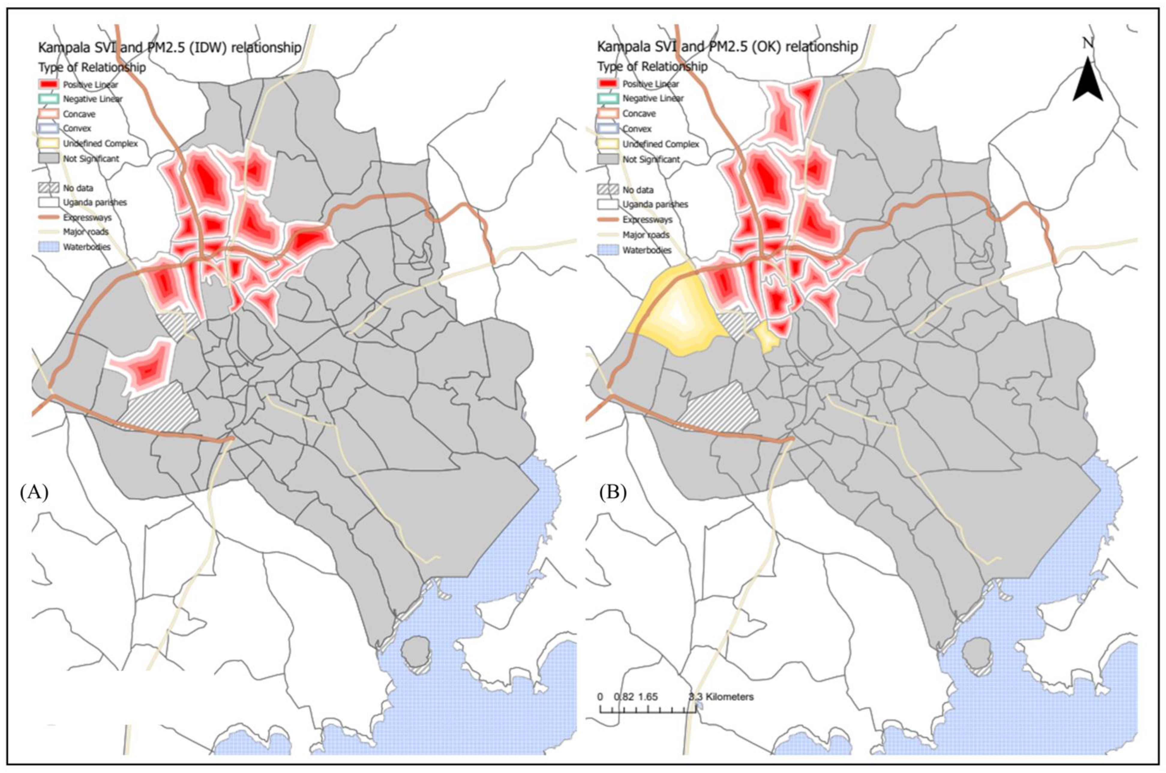
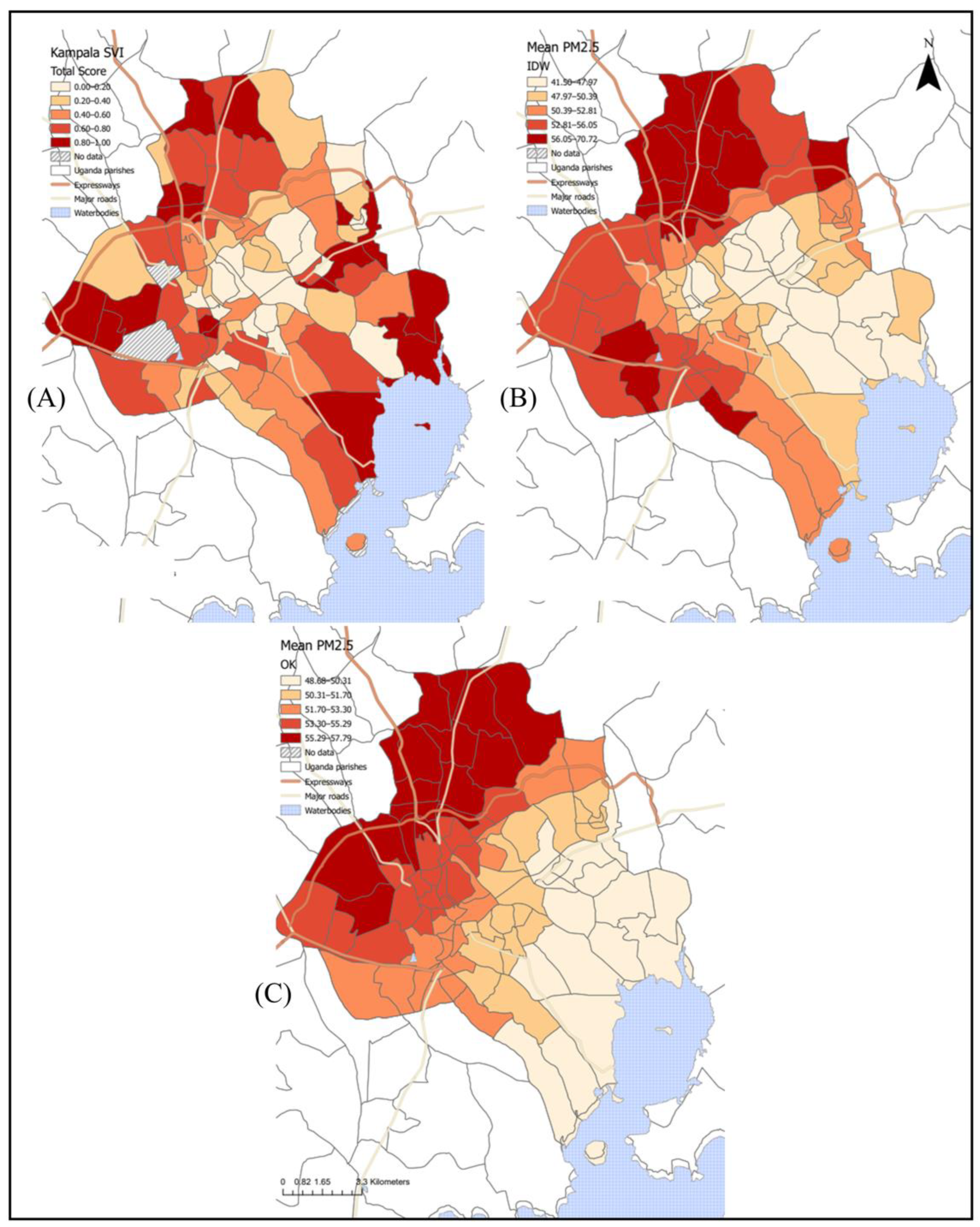
3.2. Kampala-Specific Analysis

The Kampala-specific analysis shows a more spatially refined analysis than the nationwide analysis. Figure 3A shows the SVI at the parish level for the Kampala district, the capital city of Uganda. The parishes that fall into the highest quintile (0.8 to 1) occur in the outskirts of the district. Notably, the parishes with low vulnerability significantly cluster in the central part of the district (Figure S2 of Supplementary Materials). Figure 3B shows the annual mean IDW PM2.5 concentration for 2020 in the Kampala district. The highest average yearly PM2.5 measurement was 70.72 μ g/m3, and the lowest PM2.5 yearly average was 41.50 μ g/m3. Figure 3C shows the annual mean concentration of PM2.5 for 2020 in the Kampala district using the OK. The highest average yearly PM2.5 measurement was 57.79 μ g/m3, and the lowest annual PM2.5 average was 48.58 μ g/m3. Both the IDW and OK methods show a similar pattern of higher PM2.5 in the northwestern parishes of the district (closer to major highway junctions) and lower concentrations seen in the southeastern parishes (closer to Lake Victoria).
Figure 4A,B shows the local bivariate spatial relationship between parish SVI for the Kampala district and PM2.5 concentrations estimated by IDW and OK. The IDW method identified 20 parishes with statistically significant positive linear relationships between SVI and PM2.5 concentration. The OK method identified 22 parishes with statistically significant positive linear relationships between SVI and PM2.5 concentration. Hence, these parishes face combined social and biophysical (air pollution) vulnerability.

4. Discussion

4.1. Social Vulnerability Profile and Clustering of Vulnerability across Subcounties in Uganda

Our study is the first, to our knowledge, to develop an SVI in the context of air pollution in SSA. Results of our analysis show widespread social vulnerability to air pollution throughout the country of Uganda. The themes driving the overall score included economics, housing, communication, and health, as they had similar patterns of vulnerability distribution throughout the country. Economic and communication themes comprised variables related to income and education. Income and education were the two variables used in an SVI created in Beijing. The researchers found that air quality was significantly worse where residents have low income and low education rates [39]. Additionally, these residents are usually less capable of protecting themselves from the potentially adverse health risk related to PM2.5 [39]. Embedded in the communication theme is access to information through different media, such as television and radio, as this has been shown to contribute to health recovery and well-being at the community and individual levels after natural disasters [40].
The housing theme has variables related to the materials used to build the home and the renting status of the house. In another study conducted in Uganda, property ownership was associated with social vulnerability [41]. Here, they found that owning property did not protect one from exposure to extreme climate events (flood and drought); however, it could reduce the intensity of the effects of these events [41]. The health theme has variables related to distance to health facilities and water, sanitation, and hygiene (WaSH) practices and resources. Health facility access and WaSH are important in exposure to air pollution because both have overlapping health risks with air quality, such as respiratory illnesses and childhood growth outcomes [31,42,43].
Our SVI analysis shows that the northern subcounties, which are the more rural subcounties of UG, have higher levels of social vulnerability. The social vulnerability profile also highlights that those areas experiencing low social vulnerability are more urban and developed areas, such as the capital city of Kampala, the Mbale district, and the border between Uganda and Kenya. Since colonial times, these areas have become more highly developed and are strategic because of water availability and defense [44]. This finding is similar to that of a study conducted in the US that found more significant inequalities in educational attainment and neighborhood deprivation in rural areas than in urban settings [45].
Based on the LISA, we found significant clustering of high social vulnerability in the country’s northern region at the subcounty level. These subcounties are more rural and surrounded by other subcounties with similar SVI profiles. There was significant clustering of low vulnerability in the southwestern and southeastern parts of the country. These subcounties are more urban and developed and surrounded by other subcounties with similar SVI profiles.

4.2. Association between Nationwide Estimates of PM2.5 and SVI in Subcounties in Uganda

The bivariate analysis (Figure 2B) showed that there were positive and negative linear relationships, as well as nonlinear relationships, between ambient annual PM2.5 mean concentration and SVI. Most subcounties showed that the relationship between PM2.5 and SVI were nonsignificant. The other nonlinear relationships that were specific to some subcounties highlight the fact that the PM2.5 exposure and SVI relationship is not always linear in some settings.
The subcounties with a positive linear relationship have high values of SVI and PM2.5 and are near to places where low SVI is collocated with low PM2.5 values. Areas with low–low values for both variables and a positive linear relationship are relatively safer and better able to cope with hazards.
Therefore, areas that are high–high from the LISA analysis (Figure 2A) and have a positive linear relationship from the bivariate analysis would be of particular concern. These subcounties should be prioritized for air pollution mitigation efforts as our data suggest that these are communities at greater coexposure vulnerability in terms of PM2.5 and social factors. The recommendation for policymakers would be to address social issues related to housing and access to health facilities, improve public communication, implement proper garbage disposal, and shift the main light source to one that is less polluting.

4.3. Association between In Situ Estimates of PM2.5 and SVI in Parishes in Kampala, Uganda

The smallest geographic unit that was available from the Uganda census was at the parish level, which was used to for the Kampala district, which is the capital city. The results of this analysis highlighted the heterogeneous nature of human population data [46]. Analyzing on a smaller spatial scale, it appears that there were highly vulnerable populations at the parish level within Kampala, which was not easily noted in the analysis at the subcounty level as this seemed to mask these subregional inequalities. The higher PM2.5 estimates are closer to major roads, which is expected based on other literature showing that traffic-related pollution is a major contributor of PM2.5 concentrations [47,48]. The SVI profile of this district shows that the outer parishes have higher social vulnerability, and the inner parishes have lower vulnerability (Figure 4A,B).
The positive linear relationship parishes are those that have high values of SVI and PM2.5 and are near to places where low SVI is collocated with low PM2.5 values. These parishes are those that need to be prioritized for improved social or air quality reduction intervention. These parishes can also be prioritized for having air monitoring and social interventions.

4.4. Comparison of Other Social Vulnerability and PM2.5 Studies

Other studies have shown similar relationships between SVI and PM2.5 [39,49,50,51,52,53]. One study conducted in Beijing estimated annual PM2.5 concentrations from air quality monitors stationed in the area using Ordinary Kriging and land-use regression methods by district [49]. The authors then created an inequality index that included age subgroups (≤4, 5–19, 20–59, and ≥60) and education status (illiterate, primary, secondary, and tertiary) [49]. From the index value trends, they found that annual PM2.5 exposures were disproportionately high for children (age ≤ 4) and residents with lower education [49].
A study conducted in Hong Kong focused on environmental injustice and its role in particular population members who are disproportionately affected by environmental pollution, such as poor air quality [50]. The authors created a social deprivation index using principal component analysis, which included income, education, and nonprofessional occupation taken from census data at the constituency area level [50]. They estimated the monthly PM2.5 concentration using air monitors that the local government set up in the area and the Granger causality model at the constituency area level [50]. They used ordinary least squares regression. The results showed a significant positive linear relationship between ambient PM2.5 levels and the social deprivation index [50].
Other researchers in the same area conceptualized air quality as the hazard and the capacity to cope with the associated adverse health outcomes as the risk [39]. They used three sets of data to estimate PM2.5 concentrations; one of them is the global annual PM2.5 concentration dataset provided by the Atmospheric Composition Analysis Group at Dalhousie University, Canada, which was the same dataset used in this study [39]. Pearson’s correlation coefficients were used to determine the association between PM2.5 concentration and social vulnerability [39]. Their results showed that social vulnerability is significantly associated with higher PM2.5 [39].
Despite the concepts of social vulnerability and environmental justice originating in the US, which has its unique contextual elements of structural racism and locating hazardous waste and toxic facilities in low-income communities, they have broadened to settings outside the US [54]. Researchers in the United Kingdom calculated annual PM2.5 measures from hourly values collected by the European Monitoring and Evaluation Programme (EMEP) [51]. Then they modified the 2010 English Index of Multiple Deprivation (IMD), like the SVI, which used two of the key domains: income and employment [51]. They found that the relationships between pollution levels and the 10 levels of socioeconomic deprivation were nonlinear. The concentrations of PM2.5 were similar for the first five groups of SDI (the less disadvantaged group) and then started to increase at the sixth level to the tenth level (more disadvantaged groups). They also found that the relationship varied by urban–rural status. There was a more significant disparity in PM2.5 concentration in the rural areas among the deprivation groups than in the urban area [51]. Another study, conducted in the UK, created a Multiple Environmental Deprivation Index (MEDIx) that included air pollution, climate change, industrial facilities, UV radiation, and green space. The authors related this index to two social variables, income and population density [54]. The results showed that low-income and more populated areas had worse MEDIx scores [54]. Researchers found in Australia that areas characterized by higher socioeconomic disadvantage, high proportions of ethnic minorities, and higher elderly populations also have higher ambient PM2.5 concentrations [52]. Regionally, in East Africa, researchers also found that low-income populations often reside in areas likely to have high exposure to air pollutants—low-quality housing and urban areas [53].
There are several limitations of this study that should be considered when interpreting the results. First, the modifiable areal unit problem (MAUP) can contribute to bias in inferential statistics, whereby aggregating to higher areal units may mask associations that are occurring at lower levels of areal unit aggregation [55]. We attempted to mitigate the MAUP by performing our analysis on a nationwide scale using subcounties and then on a district scale by using smaller administrative boundaries (parishes). Second, because we only used modeled PM2.5 estimates and subsequently averaged these to areal units, there is some uncertainty concerning the pollution levels analyzed.
The strengths of this research project include the data used to calculate the SVI, which was the most recent census (2014) data for the country. Therefore, the data are comparable with other research on this topic. Our study is one of the first to focus on the African continent. Further research needs to be conducted in other African countries as they are typically areas where high SVI and environmental contaminants converge. Additionally, further research needs to explore the toxic effects of pollutants in these vulnerable communities.

5. Conclusions

Using the most recent Ugandan census, global PM2.5 estimates, local PM2.5 monitoring data, and multiple geographical analyses, we were able to answer the five objectives of the study. We found that (1) several subcounties in Uganda are socially vulnerable to air pollution effects; (2) there was significant local clustering of high vulnerability in the northern region of the country and low vulnerability across subcounties in the southern and central regions of the country; (3) the nationwide scale association between spatial estimates of ambient PM2.5 and SVI in subcounties in Uganda showed that some subcounties have positive linear relationships; (4) the local-scale association between more spatially refined estimates of PM2.5 and SVI in parishes in Kampala, Uganda, showed that there was a positive linear relationship in the northern parishes of the district; and (5) several northern parishes in Kampala and northern subcounties in Uganda are areas of particular concern in Uganda as they face high social vulnerability and high PM2.5 air pollution. Moreover, our approach can be extended to other countries in Africa to help prioritize communities in need of air pollution monitoring and air pollution mitigation.

Supplementary Materials

The following supporting information can be downloaded at: https://www.mdpi.com/article/10.3390/atmos13081169/s1, Document S1: Example of percentile rank calculation; Figure S1: Spatial Autocorrelation Report (Moran’s I); Figure S2: Local indicators of spatial autocorrelation (LISA) for Kampala.

Author Contributions

Conceptualization, K.C., K.A., E.S.C. and E.B.; methodology, K.C., K.A., E.S.C. and E.B.; writing—original draft preparation, K.C., E.S.C. and K.A.; writing—review and editing, K.A., E.S.C., T.S.-A. and E.B.; supervision, K.A., E.S.C. and E.B.; funding acquisition, E.B. All authors have read and agreed to the published version of the manuscript.

Funding

The AirQo project was funded by a grant from Google.org, Sida, IDRC, Enabel/Wehubit, and EPSRC.

Institutional Review Board Statement

Ethical review and approval were waived for this study due to the fact that all data used in this study is publicly available and the original data is properly anonymized.

Informed Consent Statement

Not applicable.

Data Availability Statement

The data generated and analyzed in this study are available upon request from the corresponding author.

Acknowledgments

Special acknowledgements go to the AirQo project for providing low-cost air quality monitoring data for Kampala.

Conflicts of Interest

The authors declare no conflict of interest. The funders had no role in the design of the study; in the collection, analyses, or interpretation of data; in the writing of the manuscript; or in the decision to publish the results.

References

  1. Bauer, S.E.; Im, U.; Mezuman, K.; Gao, C.Y. Desert dust, industrialization, and agricultural fires: Health impacts of outdoor air pollution in africa. J. Geophys. Res. Atmos. 2019, 124, 4104–4120. [Google Scholar] [CrossRef]
  2. Abera, A.; Friberg, J.; Isaxon, C.; Jerrett, M.; Malmqvist, E.; Sjöström, C.; Taj, T.; Vargas, A.M. Air quality in africa: Public health implications. Annu. Rev. Public Health 2021, 42, 193–210. [Google Scholar] [CrossRef] [PubMed]
  3. WHO HIV/AIDS | WHO | Regional Office for Africa. Available online: https://www.afro.who.int/health-topics/hivaids (accessed on 4 May 2022).
  4. IHME Global Burden of Disease Visualisations: Compare. Available online: https://www.thelancet.com/lancet/visualisations/gbd-compare (accessed on 4 May 2022).
  5. EPA Health and Environmental Effects of Particulate Matter (PM) | US EPA. Available online: https://www.epa.gov/pm-pollution/health-and-environmental-effects-particulate-matter-pm (accessed on 4 August 2021).
  6. Backus, L.I.; Boothroyd, D.; Deyton, L.R. HIV, hepatitis C and HIV/hepatitis C virus co-infection in vulnerable populations. AIDS 2005, 19, S13–S19. [Google Scholar] [CrossRef] [PubMed]
  7. Garlick, D. The vulnerable people in emergencies policy: Hiding vulnerable people in plain sight. Aust. J. Emerg. Manag. 2015, 30, 31–34. [Google Scholar]
  8. Brooks, N. Vulnerability, Risk and Adaptation: A Conceptual Framework. Available online: https://www.researchgate.net/publication/200032746 (accessed on 27 April 2022).
  9. Yang, X.; Geng, L.; Zhou, K. The construction and examination of social vulnerability and its effects on PM2.5 globally: Combining spatial econometric modeling and geographically weighted regression. Environ. Sci. Pollut. Res. Int. 2021, 28, 26732–26746. [Google Scholar] [CrossRef]
  10. Yang, X.; Geng, L.; Zhou, K. Environmental pollution, income growth, and subjective well-being: Regional and individual evidence from China. Environ. Sci. Pollut. Res. Int. 2020, 27, 34211–34222. [Google Scholar] [CrossRef]
  11. Aksha, S.K.; Juran, L.; Resler, L.M.; Zhang, Y. An Analysis of Social Vulnerability to Natural Hazards in Nepal Using a Modified Social Vulnerability Index. Int. J. Disaster Risk Sci. 2019, 10, 103–116. [Google Scholar] [CrossRef] [Green Version]
  12. Karaye, I.M.; Horney, J.A. The Impact of Social Vulnerability on COVID-19 in the U.S.: An Analysis of Spatially Varying Relationships. Am. J. Prev. Med. 2020, 59, 317–325. [Google Scholar] [CrossRef]
  13. Strader, S.M.; Haberlie, A.M.; Loitz, A.G. Assessment of NWS County Warning Area Tornado Risk, Exposure, and Vulnerability. Weather Clim. Soc. 2021, 13, 189–209. [Google Scholar] [CrossRef]
  14. Tate, E.; Rahman, M.A.; Emrich, C.T.; Sampson, C.C. Flood exposure and social vulnerability in the United States. Nat. Hazards 2021, 106, 435–457. [Google Scholar] [CrossRef]
  15. Largest Countries in Africa 2022. Available online: https://worldpopulationreview.com/country-rankings/largest-countries-in-africa (accessed on 27 April 2022).
  16. CIA Uganda-The World Factbook. Available online: https://www.cia.gov/the-world-factbook/countries/uganda/ (accessed on 11 July 2021).
  17. World Bank Group Uganda Overview. Available online: https://www.worldbank.org/en/country/uganda/overview (accessed on 11 July 2021).
  18. Makita, K.; Fèvre, E.M.; Waiswa, C.; Bronsvoort, M.D.C.; Eisler, M.C.; Welburn, S.C. Population-dynamics focussed rapid rural mapping and characterisation of the peri-urban interface of Kampala, Uganda. Land Use Policy 2010, 27, 888–897. [Google Scholar] [CrossRef] [PubMed] [Green Version]
  19. Petkova, E.P.; Jack, D.W.; Volavka-Close, N.H.; Kinney, P.L. Particulate matter pollution in African cities. Air Qual. Atmos. Health 2013, 6, 603–614. [Google Scholar] [CrossRef]
  20. WHO Ambient (Outdoor) Air Pollution. Available online: https://www.who.int/news-room/fact-sheets/detail/ambient-(outdoor)-air-quality-and-health (accessed on 13 July 2021).
  21. Coker, E.S.; Amegah, A.K.; Mwebaze, E.; Ssematimba, J.; Bainomugisha, E. A land use regression model using machine learning and locally developed low cost particulate matter sensors in Uganda. Environ. Res. 2021, 199, 111352. [Google Scholar] [CrossRef] [PubMed]
  22. UBOS Explore Statistics–Uganda Bureau of Statistics. Available online: https://www.ubos.org/explore-statistics/20/ (accessed on 2 December 2021).
  23. OCHA Uganda-Subnational Administrative Boundaries-Humanitarian Data Exchange. Available online: https://data.humdata.org/dataset/uganda-administrative-boundaries-admin-1-admin-3 (accessed on 14 January 2022).
  24. Ge, Y.; Zhang, H.; Dou, W.; Chen, W.; Liu, N.; Wang, Y.; Shi, Y.; Rao, W. Mapping social vulnerability to air pollution: A case study of the yangtze river delta region, china. Sustainability 2017, 9, 109. [Google Scholar] [CrossRef] [Green Version]
  25. Gupta, S.; Das, S.; Murty, M.N. Quantifying air pollution vulnerability and its distributional consequences. Ecol. Econ. Soc. 2019, 2, 93–125. [Google Scholar] [CrossRef]
  26. Muyanja, D.; Allen, J.G.; Vallarino, J.; Valeri, L.; Kakuhikire, B.; Bangsberg, D.R.; Christiani, D.C.; Tsai, A.C.; Lai, P.S. Kerosene lighting contributes to household air pollution in rural Uganda. Indoor Air 2017, 27, 1022–1029. [Google Scholar] [CrossRef]
  27. Richmond, A.; Myers, I.; Namuli, H. Urban informality and vulnerability: A case study in kampala, uganda. Urban Sci. 2018, 2, 22. [Google Scholar] [CrossRef] [Green Version]
  28. Coker, E.; Katamba, A.; Kizito, S.; Eskenazi, B.; Davis, J.L. Household air pollution profiles associated with persistent childhood cough in urban Uganda. Environ. Int. 2020, 136, 105471. [Google Scholar] [CrossRef]
  29. Tate, E. Social vulnerability indices: A comparative assessment using uncertainty and sensitivity analysis. Nat. Hazards 2012, 63, 325–347. [Google Scholar] [CrossRef]
  30. Flanagan, B.E.; Gregory, E.W.; Hallisey, E.J.; Heitgerd, J.L.; Lewis, B. A social vulnerability index for disaster management. J. Homel. Secur. Emerg. Manag. 2011, 8, 0000102202154773551792. [Google Scholar] [CrossRef]
  31. Clasen, T.; Smith, K.R. Let the “A” in WASH Stand for Air: Integrating Research and Interventions to Improve Household Air Pollution (HAP) and Water, Sanitation and Hygiene (WaSH) in Low-Income Settings. Environ. Health Perspect. 2019, 127, 25001. [Google Scholar] [CrossRef] [PubMed] [Green Version]
  32. Uganda Bureau of Statistc. The National Population and Housing Census 2014—Housing and Household Conditions Report, Kampala, Uganda. 2019. Available online: http://www.ubos.org/wp-content/uploads/publications/09_2019Housing_Monograph_-_FINAL.pdf (accessed on 27 April 2022).
  33. Hammer, M.S.; van Donkelaar, A.; Li, C.; Lyapustin, A.; Sayer, A.M.; Hsu, N.C.; Levy, R.C.; Garay, M.J.; Kalashnikova, O.V.; Kahn, R.A.; et al. Global Estimates and Long-Term Trends of Fine Particulate Matter Concentrations (1998–2018). Environ. Sci. Technol. 2020, 54, 7879–7890. [Google Scholar] [CrossRef] [PubMed]
  34. van Donkelaar, A.; Martin, R.V.; Brauer, M.; Kahn, R.; Levy, R.; Verduzco, C.; Villeneuve, P.J. Global estimates of ambient fine particulate matter concentrations from satellite-based aerosol optical depth: Development and application. Environ. Health Perspect. 2010, 118, 847–855. [Google Scholar] [CrossRef] [PubMed] [Green Version]
  35. Brauer, M.; Freedman, G.; Frostad, J.; van Donkelaar, A.; Martin, R.V.; Dentener, F.; van Dingenen, R.; Estep, K.; Amini, H.; Apte, J.S.; et al. Ambient air pollution exposure estimation for the global burden of disease 2013. Environ. Sci. Technol. 2016, 50, 79–88. [Google Scholar] [CrossRef]
  36. Okure, D.; Ssematimba, J.; Sserunjogi, R.; Gracia, N.L.; Soppelsa, M.E.; Bainomugisha, E. Characterization of Ambient Air Quality in Selected Urban Areas in Uganda Using Low-Cost Sensing and Measurement Technologies. Environ. Sci. Technol. 2022, 56, 3324–3339. [Google Scholar] [CrossRef]
  37. Zonal Statistics as Table (Spatial Analyst)—ArcGIS Pro | Documentation. Available online: https://pro.arcgis.com/en/pro-app/2.8/tool-reference/spatial-analyst/zonal-statistics-as-table.htm (accessed on 9 May 2022).
  38. ArcGIS Pro Local Bivariate Relationships (Spatial Statistics). Available online: https://pro.arcgis.com/en/pro-app/2.8/tool-reference/spatial-statistics/localbivariaterelationships.htm (accessed on 15 July 2022).
  39. Huang, G.; Zhou, W.; Qian, Y.; Fisher, B. Breathing the same air? Socioeconomic disparities in PM2.5 exposure and the potential benefits from air filtration. Sci. Total Environ. 2019, 657, 619–626. [Google Scholar] [CrossRef]
  40. Hugelius, K.; Adams, M.; Romo-Murphy, E. The power of radio to promote health and resilience in natural disasters: A review. Int. J. Environ. Res. Public Health 2019, 16, 2526. [Google Scholar] [CrossRef] [Green Version]
  41. Cooper, S.J.; Wheeler, T. Rural household vulnerability to climate risk in Uganda. Reg. Environ. Chang. 2017, 17, 649–663. [Google Scholar] [CrossRef]
  42. Aghasili, O.U. Fuel choice, acute respiratory infection and child growth in Uganda. Open Access Theses 2015, 564, 1–83. [Google Scholar]
  43. Heft-Neal, S.; Burney, J.; Bendavid, E.; Burke, M. Robust relationship between air quality and infant mortality in Africa. Nature 2018, 559, 254–258. [Google Scholar] [CrossRef]
  44. Uganda Local Government Overview | Mbale District. Available online: https://www.mbale.go.ug/lg/overview (accessed on 5 May 2022).
  45. Deziel, N.C.; Warren, J.L.; Bravo, M.A.; Macalintal, F.; Kimbro, R.T.; Bell, M.L. Assessing community-level exposure to social vulnerability and isolation: Spatial patterning and urban-rural differences. J. Expo. Sci. Environ. Epidemiol. 2022. [Google Scholar] [CrossRef] [PubMed]
  46. Malleson, N.; Steenbeek, W.; Andresen, M.A. Identifying the appropriate spatial resolution for the analysis of crime patterns. PLoS ONE 2019, 14, e0218324. [Google Scholar] [CrossRef] [PubMed]
  47. Fang, X.; Li, R.; Xu, Q.; Bottai, M.; Fang, F.; Cao, Y. A Two-Stage Method to Estimate the Contribution of Road Traffic to PM2.5 Concentrations in Beijing, China. Int. J. Environ. Res. Public Health 2016, 13, 124. [Google Scholar] [CrossRef] [PubMed]
  48. Kinney, P.L.; Gichuru, M.G.; Volavka-Close, N.; Ngo, N.; Ndiba, P.K.; Law, A.; Gachanja, A.; Gaita, S.M.; Chillrud, S.N.; Sclar, E. Traffic impacts on PM2.5 air quality in nairobi, kenya. Environ. Sci. Policy 2011, 14, 369–378. [Google Scholar] [CrossRef] [PubMed] [Green Version]
  49. Ouyang, W.; Gao, B.; Cheng, H.; Hao, Z.; Wu, N. Exposure inequality assessment for PM2.5 and the potential association with environmental health in Beijing. Sci. Total Environ. 2018, 635, 769–778. [Google Scholar] [CrossRef]
  50. Li, V.O.; Han, Y.; Lam, J.C.; Zhu, Y.; Bacon-Shone, J. Air pollution and environmental injustice: Are the socially deprived exposed to more PM2.5 pollution in Hong Kong? Environ. Sci. Policy 2018, 80, 53–61. [Google Scholar] [CrossRef]
  51. Milojevic, A.; Niedzwiedz, C.L.; Pearce, J.; Milner, J.; MacKenzie, I.A.; Doherty, R.M.; Wilkinson, P. Socioeconomic and urban-rural differentials in exposure to air pollution and mortality burden in England. Environ. Health 2017, 16, 104. [Google Scholar] [CrossRef] [Green Version]
  52. Cooper, N.; Green, D.; Knibbs, L.D. Inequalities in exposure to the air pollutants PM2.5 and NO2 in Australia. Environ. Res. Lett. 2019, 14, 115005. [Google Scholar] [CrossRef]
  53. Avis, W.; Khaemba, W. Vulnerability and Air Pollution. ASAP—East Africa Rapid Literature Review. Birmingham, UK: University of Birmingham. Available online: https://sciwheel.com/work/item/12119363/resources/14843553/pdf (accessed on 27 April 2022).
  54. Pearce, J.R.; Richardson, E.A.; Mitchell, R.J.; Shortt, N.K. Environmental justice and health: The implications of the socio-spatial distribution of multiple environmental deprivation for health inequalities in the United Kingdom. Trans. Inst. Br. Geogr. 2010, 35, 522–539. [Google Scholar] [CrossRef] [Green Version]
  55. Buzzelli, M. Modifiable areal unit problem. In International Encyclopedia of Human Geography; Elsevier: Amsterdam, The Netherlands, 2020; pp. 169–173. ISBN 9780081022962. [Google Scholar]
Figure 1. (A) Map of Uganda showing the total SVI scores by subcounty. SVI is classified as quintiles. (B) Annual mean PM2.5 concentrations for the year 2014 using global estimates from the ACAG dataset also classified as quintiles.
Atmosphere 13 01169 g001
Figure 2. (A) Results of the LISA analysis of where the significant clusters are located by district for the total SVI scores. (B) Association between annual mean PM2.5 levels and total SVI scores from the bivariate analysis results.
Atmosphere 13 01169 g002
Figure 3. (A) Map of Kampala showing the total SVI scores by parish. SVI is mapped by quintiles 0 representing the lowest vulnerable districts and 1 showing the highest vulnerable areas. (B) Annual mean PM2.5 concentrations for the year 2020 using ground monitoring data from the AirQo system and the inverse distance weighting (IDW) methodology and classified using quintiles. (C) Annual mean PM2.5 concentrations for the year 2020 using ground monitoring data from the AirQo system and the Ordinary Kriging (OK) methodology also classified using quintiles.
Atmosphere 13 01169 g003
Figure 4. (A) Map of Kampala showing the association between annual mean PM2.5 levels based on inverse distance weighting (IDW) and total SVI scores from the bivariate analysis results. (B) Association between annual mean PM2.5 levels based on Ordinary Kriging (OK) and total SVI scores from the bivariate analysis results.
Atmosphere 13 01169 g004
Table 1. List of variables and themes used to create Uganda’s air pollution SVI.
ThemeVariableDefinition
Age dependencyYouth dependency ratioThe ratio of those aged 0–4 years to the population aged between 15 and 64 years
Old-age dependency ratioThe ratio of those aged 65 years and above to the population aged between 15 and 64 years
SocialChildren 0–17 who lost at least one parentPercentage of children (0–17 years old) who have lost a parent
2 years plus with disabilityPercentage of individuals who are 2 years old and above who live with a disability
50 years plus widowedPercentage of individuals who are 50 years old and above and are widowed against the total adult population
HousingTemporary dwelling unitPercentage of total households that live in units that are built using temporary materials for the roof, wall, and floor
Households that are renter occupiedPercentage of total households that are renter occupied
Inverse of the variable “households that are owner occupied” used
HealthDistance to any health facility (5 km or more)Percentage of total households that live more than 5 km away from the nearest health facility
Do not have access to piped waterPercentage of total households that do not have access to piped water
Inverse of the variable “access to piped water” used
Without access to boreholePercentage of total households that do not have access to borehole (well-water source)
Inverse of the variable “with access to borehole” used
Without any toilet facilityPercentage of total households that do not have any toilet facility
Inverse of the variable “with any toilet facility” used
Households that (all members aged 5+ years) consume fewer than two meals a dayPercentage of total households where members who are 5 years old and above consume fewer than two meals a day
CommunicationHouseholds that do not own a television (TV)Percentage of total households that do not own a TV
Households that do not own a radioPercentage of total households that do not own a radio
Population 18+ illiteratePercentage of the adult population (18+) that is illiterate
Economy18 years plus not workingPercentage of the adult population (18 years and above) that does not work
Inverse of the variable “working 18 years and older” used
Households where no member possesses a bank accountPercentage of total households where no member has a bank account
Inverse of the variable “households where any member possesses a bank account” used
Households depending on subsistence farmingPercentage of total households that depend on subsistence farming (farmers grow enough to feed their families, not to make a profit)
Air qualityHouseholds that do not properly dispose of solid wastePercentage of total households that do not dispose of solid waste properly
Inverse of the variable “households that properly dispose of solid waste” used
Households’ main source of lighting is tadoobaPercentage of total households that use tadooba (a thick-wick lamp) as their main source of lighting
Households using polluting fuel for cookingPercentage of households that use polluting fuel (paraffin, firewood and charcoal, grass or cow dung, and others)
Publisher’s Note: MDPI stays neutral with regard to jurisdictional claims in published maps and institutional affiliations.

