1. Introduction
Precipitating weather systems, and the frequently catastrophic phenomena that might accompany them, have a direct impact on humans as they affect a number of activities, e.g., agriculture, transport, construction, etc. Precipitation and knowledge of the time of its occurrence, location and intensity, are important and make a forecast useful and successful. Rain is a parameter that varies significantly in space and time and is greatly influenced by topography and other geophysical features. Therefore, simulations with very high-resolution numerical models that have the ability to take into account small-scale factors are of primary importance foraccurate forecast. Although the increase in computing power has made it possible to have operational numerical forecasts at kilometer (km) resolution scale leading to forecasts in terms of the spatial structure of the precipitation, nevertheless they often suffer from errors that develop rapidly on small scales [
1]. Factors that contribute to the deviations of rainfall forecasts are related to the initial conditions, to the errors in the replication of the atmospheric dynamics as well as to the inadequacy of microphysical schemes in the calculation or parameterization of both large-scale and convective precipitation. As a result, there is a natural limit in the predictability of models that needs to be analyzed and quantified through an ongoing evaluation process.
Objective evaluation of precipitation forecasts with detailed structural features as well as intensity gradients over short spatio-temporal periods is a demanding process and requires a high-resolution representation of actual conditions that is often not available. Usually incomplete ground observation data, lower spatial resolution rainfall estimates from remote sensing or unrealistically interpolated observation fields with low accuracy are the choices of “truth” that will determine the degree of predictability of precipitation forecasts. The need to find scientifically substantiated proposals to address the daily challenges in the field of forecast verification have provided the impetus for this study.
Precipitation verification is an integral part of meteorological research activities, but it should also feature in operational forecasting, as it is the element that essentially determines the competency of an NWP system. If the evaluation methodology is properly designed, the verification results can effectively meet the needs of many different groups, including model developers, researchers, forecasters, and end users of meteorological products. In general, the vast majority of precipitation verification efforts by meteorological services focuses on the calculation of one or more statistical indicators based on limited sets of forecast-observation data. These methods are referred to as “traditional” to distinguish them from the latest developments in verification techniques. Research and development of new verification approaches has advanced significantly in recent decades and has been driven by various factors, such as the availability of new sources of precipitation data from remote sensing (satellite and radar estimates) and the production of ultra-high-resolution numerical forecasts. Thorough verification involves evaluating characteristics such as the location of a weather system, the shape and size of rain formations, the breadth of coverage and the intensity of the parameter. Spatial verification methods make it possible to attribute the physical dimension of the error, relaxing the need for point-to-point comparisons, thus providing additional information to the results of traditional verification techniques [
2].
The next challenge in the implementation of a forecast evaluation system is to obtain a detailed description of the “actual” state of the atmosphere. This needs to be available in the same spatio-temporal detail as the numerical forecast, in particular for the application of spatial verification methods. For precipitation, ground observation networks are insufficient and usually not representative of the whole geographical area of interest, especially in areas at high altitude with steep slopes, which are characteristic of all observation networks in Greece. At the same time, only a small fraction of the observations is currently used in verification procedures at most forecasting centers. This is due to the difficulty of retrieving and collating such data, performing the necessary quality control and processing of data before use. These factors often lead to the use of model analysis from data assimilation systems as the “truth” for operational verification applications, instead of “raw” data observations. Such analyses have the advantage of maintaining the physical coherence of the model and are therefore characterized by a temporal and spatial structure. However, they tend to filter and smooth the observation data through the assimilation process. Remote sensing, on the other hand, has greatly assisted in the implementation of high-resolution precipitation applications, but the resolution of observations is often lower and, most importantly, the measurement is not direct. Satellite data and even radar recordings are estimates with a degree of uncertainty that makes it difficult to capture the objective reality of the precipitation field. Therefore, it is necessary to assess and adopt methods that include various sources of observations for the construction of rain observations with both high resolution and reliability at regular intervals.
In this study, an interpolation method based on climatology is used to estimate the distribution of precipitation observations on various timescales. The idea behind this method stems from the principles that gridded data of a higher quality can be resulted when correlated with certain climatological statistical parameters (such as geophysical characteristics), which can be modelled using long climate data series while remote sensing precipitation estimates are added as background information, which in turn is evaluated in combination with the interpolated value. Subsequently, the precipitation forecasts are assessed using various spatial methods in an effort to identify the ability of each verification approach to provide distinctly useful information on model performance. Finally, the development of an integrated verification system for precipitation forecasts is proposed that meets the requirements of an operational system and is adapted to the specificities of the Greek territory.
2. Materials and Methods
2.1. Climatological Characteristics of Area of Interest
Although precipitation is directly related to atmospheric disturbances, it is strongly influenced by local orographic effects. In Greece, the mainland occupies about 80% of the total area of the country. The remaining 20% is distributed among about 6000 islands and islets. The landscape is mainly mountainous and hilly, with a strong relief in both the horizontal and vertical. The maximum altitude reaches 2918 m above sea level. The western part of the mainland is mountainous with few plains. Most of the plains are located on the east side of the country, often close to the coastline. According to Flocas [
3], the low (0–200 m) and medium-high (201–500 m) altitude areas correspond to 32.8% and 26.0%, while the semi-mountainous (501–1000 m) and mountainous areas (1001–1500 m) correspond to 27.8% and 9.9% of the total area, respectively. The remaining 3.5% corresponds to the subalpine (1501–2000 m) and alpine (over 2000 m) areas.
Precipitation in the national network is recorded with standard rain gauges, in some areas by the available radar network, while satellite rainfall estimation data are also available with the advantage that they cover the entire geographical area. From the analysis of the mean precipitation climatological values [
4], the rain caused by the Pindos Mountain range on the mainland, as well as that caused by the mountains of the Peloponnese dominate the annual rainfall totals. The rain shadow phenomenon results in the highest precipitation values occurring in the areas west of Pindos and in Western Greece, and to a lesser extent in central and eastern Greece and the Cyclades. In Greece, due to the complex terrain and the insufficient network of ground observations, any attempt to measure the actual rainfall field at regular time intervals with a high enough spatial resolution is a demanding process. Therefore, the need for continuous and detailed spatio-temporal realistic monitoring of rain over Greece for use in the evaluation of numerical forecasts requires a process of utilizing all existing sources of observations in the best possible way.
2.2. Gridded Precipitation Observations
The ability to provide meteorological information in areas where observations are not available is of primary importance. Efforts to document geographically distributed precipitation have been underway for many decades. Historically available surface observation files and gridded products are complemented by the increasing potential of remote sensing observations [
5]. While spatial analysis of large-scale monthly observations is well established, relatively recent advances in meteorological data interpolation methods make it possible to address new challenges regarding the representation of rainfall in high spatio-temporal resolution. One such approach, which is the subject of this work, is the creation of gridded data that will allow a more spatially realistic representation of precipitation for use in the evaluation of NWP hourly or daily cumulative precipitation forecasts.
There are several factors to consider when you need to spatially interpolate meteorological data in order to choose the appropriate method. When the spatial distance between the observation stations is large, the quality of the interpolation outcome can be improved by using a method that uses covariates to compensate for the low density of the stations. This is especially true for precipitation, as such approaches have been shown to significantly improve the representation of its spatial structure [
6]. Additionally, covariates are often available in high resolution compared to the variables that need to be interpolated [
7]. It is important, however, that a good correlation exists between the covariate and variable, i.e., precipitation in this case. This is usually evaluated using regression analysis. The variables used in this approach are geostatistical parameters related to spatial parameters that affect the meteorological parameter being analyzed [
8].
Physical factors are of primary importance when selecting the precipitation related variables. In general, atmospheric circulation characteristics, such as the position and orbit of a low pressure system or the direction of the prevailing wind, contribute to the local climate and are factors that are reflected in the observation data for a specific location [
9]. Other determinants that affect the local climate are the presence of natural features, such as large bodies of water that provide a source of moisture as well as topographic features that affect wind flow. Altitude can also have a large effect on rainfall due to orographic effects [
10,
11]. In most cases, rainfall increases with altitude through the process of elevation, adiabatic cooling and the resulting condensation of air in the windward areas of the mountains [
12], while the opposite effect is observed in the leeward [
13]. The complex geographical characteristics of Greece, as described in previous paragraph, are dominated by both the sea and the intense topography which make it difficult to capture small scale rain characteristics with its moderately dense network of rain gauges. Therefore, the gridded precipitation fields must be derived from observations at different altitudes and be evenly distributed with respect to the physical characteristics of the area of interest.
Efforts to produce realistic gridded precipitation fields based on long timeseries of observations are relatively limited in the Eastern Mediterranean region and especially in Greece. Feidas et al. [
14] extensively examined the possibility of using various geographical and topographic parameters in a multiple regression analysis to model and map the spatial variation of climatological temperature and rainfall values. Altitude, distance from the coastline and especially the distance from the Aegean Sea are important factors that affect precipitation regimes over Greece, however, the correction of the regression models using residuals was not shown to significantly improve accuracy. There is no indication regarding what the most appropriate method for the analysis of rain observations may be. The choice of method depends on the meteorological process to be analyzed, the available information, the spatial and temporal scales, the level of accuracy required and even on the computational requirements for its application.
2.2.1. MISH Methodology
In the present work it was decided to use the MISH (Meteorological Interpolation based on Surface Homogenized data basis) interpolation method. MISH was used for the creation of gridded data based on homogenized observations developed specifically for meteorological purposes [
15,
16]. The main advantage of MISH is that it can derive valuable climate information from long-term precipitation data series by calculating certain statistical parameters used in the interpolation formulae. It consists of two components: the modeling and the interpolation components.
The MISH modeling process is very time consuming but is only performed once (for each month of the year) before the interpolation applications of any precipitation dataset. On the other hand, interpolation can be used for hourly, daily, monthly, or annual values with the results of the modeling. Since the modeled interpolation parameters are obtained for a spatially dense matrix (<1 km), relatively few dependent variables (predictors) are needed for the interpolation process for any given set of observations.
This method was already successfully applied for the development of gridded climatological temperature and precipitation data in Greece [
4,
17]. In the current study, the modelling component products of MISH for precipitation are used as derived by Gofa et al. [
4]. Specifically, during the modeling phase, a multiplicative model was applied to estimate precipitation values from optimum model deterministic variables on a monthly basis. The model was based on long-term homogenized precipitation data series and supplementary geophysical variables. Regarding the geophysical variables, 20 independent geophysical variables were used as predictors of monthly precipitation values. A detailed explanation of the variables that proved to be more relevant to the topographic influence on climate data is given by Mamara et al. [
17]. These variables were: the elevation derived from a 90 m digital elevation model (DEM) originating from the NASA Shuttle Radar Topography Mission (SRTM), the first 15 principal components (PCs) proposed by the Analyse Utilisant le RELief pour les besoins del’ HYdrométéorologie (AURELHY) method [
18], latitude, incoming solar irradiance, the Euclidian distance from the coastline, and the land-to-sea percentage. The modeling phase resulted in an optimum number of variables used per month as precipitation predictions that was less than six, with the elevation proving to be the most well correlated independent variable in all cases while the land-sea percentage and some of AURELHY principal components were also included in these six most well correlated geophysical parameters [
4].
For its second software component, MISH has two types of interpolation formulas: an additive (e.g., temperature) or multiplicative (e.g., precipitation) model and formula can be used depending on the elements. In this study, only the multiplicative interpolation formula was used for the interpolation of precipitation due to its quasi-lognormal probability distribution. During the generation of gridded observations, hourly or daily precipitation values were interpolated using an adequate number of predictors as determined by the modelling component, while the interpolation error was modelled by substituting the modelled optimum interpolation parameters and the predictor values into the interpolation formulae [
15]. Both modelling and interpolation components were generated in a domain covering Greece with a 30″ (0.0083333°) resolution, which corresponds to approximately 730 m at 38° N.
2.2.2. Gridded Observations with Use of Background
Although the MISH interpolation component derived from sparse point ground observations may be sufficient when mapping average monthly climatological values, it is necessary to enrich the process with additional data in order to produce high spatiotemporal analysis of rainfall observations. This is especially crucial during the evolution of a weather system, especially over maritime areas or over the sharp terrain of Greece. MISH provides the ability to integrate background fields, such as NWP model output, satellite and radar data, which can be used to effectively reduce interference error.
Assuming that matrix
B (
s,
t) (s ∈ D: MISH grid) contains the background data within a dense grid embedded in the MISH modeling grid, the linear regression model applied for the predictands (observations) and the background is:
where
Z(
s,
t) are independent estimators (predictors),
β0(
t),
β1(
t) are the parameters to be estimated,
E(
s) is the spatial tendency and
ε(
s) is the term indicating the error of interpolation. The correlation:
describes the stochastic interconnections between the measurements and the background field. The larger the
R(
t), the more accurate the interpolation will be. In the special case that
R(
t) = 0, then there is no stochastic connection between the measurements and the background information, consequently it is not used by the software. Conversely, when
R(
t) = 1, then the interpolated value is equal to that of the background field. In all intermediate cases, the value of the interpolation will be calculated by:
where
ZB is the unknown predictant, the first term concerns the interpolation without background, while the second term is connected with the interpolation of the background information [
13].
Only one background field can be ingested during each application of MISH interpolation module. Radar data that are used in this proposed evaluation framework provide real-time automated reflectivity recordings that are updated every 7.5 min at twelve Plan Position Indicator (PPI) elevations with a horizontal resolution of 400 m. Satellite estimates of rainfall intensity that are used in the applications are retrieved from the H-SAF (EUMETSAT Satellite application Facility on Support to Operational Hydrology and Water Management) products. In particular, the precipitation product H05 was used, which is the cumulative rainfall on the surface (available at intervals of 3, 6, 12 and 24 h) from mixing the data from LEO/MW (low Earth Orbit/Microwave) and GEO/IR (Geosynchronous Earth Orbit/Infrared) supported by precipitation analyses (NWP first guess-first guess, rain meters) and an appropriate statistical correction [
19]. The product was produced with a spatial resolution of 8 km in the coverage area of H-SAF. Finally, the satellite data is available in a native projection system in a grid format, roughly in line with SEVIRI’s grid over Europe. Based on product evaluation reports [
20,
21], the precipitation product H05 has a tendency to understate high rainfall amounts (high intensity of the phenomenon). Since the objective of this study was not to estimate errors in rainfall estimates from satellite observations but to use them as background data in an attempt to cover areas where no measurements from rain gauges (mountain and sea) were available, the accuracy of the data was considered satisfactory while the impact of their use in the production of gridded observations was evaluated in detail for each experimental case.
2.3. Spatial Verification Methods
As mentioned above, there is a clear need for verification techniques that allow for some tolerance of small errors and deviations both in space and time in the numerical forecasts of precipitation [
22]. For numerical models with a spatial resolution of less than 3 km, the deep convection parameterization is no longer necessary. This allows the explicit s2imulation of convection phenomena caused either by fronts or by synoptic scale forcing, resulting in the most realistic forecast of the precipitation [
23]. To overcome the problems of double error, a new generation of spatial verification methods has been developed in recent decades in parallel with the evolution of numerical forecasting. A large number of spatial verification methods with more relaxed criteria in the comparison of forecast and observation fields were developed for the needs of objective evaluation as described by Brown et al. [
24] and Gilleland et al. [
25]. The spatial methods can be classified into the following groups: A.
filtering approaches that include: (i)
neighborhood methods that provide values for spatially and/or temporally approximated forecasts and (ii)
scale separation methods that isolate scale-dependent errors, B.
displacement approaches that include: (iii)
object based methods that evaluate their characteristics and finally (iv)
field distortion methods that calculate phase errors and parameter amplitude [
26]. The choice of the appropriate approach depends on the nature of the forecasting system and the questions to be answered regarding the quality of the forecasted parameter [
27].
The primary purpose of operational verification of precipitation fields in a national meteorological service (NMS) concerns the monitoring of developments in the NWP chains used and their evaluation to find systematic errors, to quantify the range of these errors but also to highlight the quality characteristics of the various forecast products [
28]. The evaluation process can provide valuable information to all stakeholders, such as modelers, researchers, forecasters, and the public who use the products of an NMS. Newer spatial verification methods are generally more complex to compute than traditional point methods, and the results (statistical quantities) produced are often more difficult to interpret. A comprehensive verification framework should include both traditional techniques with point-to-point comparison between observations and forecasts, and a limited number of spatial methods that can provide useful information on the short-term predictive skill of numerical simulations but also information on their reliability over a wide geographical area, time period, and different weather regimes. The development and free distribution of software packages that allow the implementation of spatial methods, such as the Model Evaluation Tools (MET) developed by the National Center for Atmospheric Research (NCAR) [
29] and the SpatialVx statistical package in R language [
30] have played an important role in their increasing use. Significant emphasis should be placed on addressing issues related to large data volume management and simulation time that may not meet the requirements of operational verification.
The spatial methods that were selected from the plethora of available ones to be components of a systematic framework for evaluating numerical precipitation forecasts, are those that are acceptable in terms of the required simulation time, namely intuitive user-oriented statistical indices that belong to the two major categories of filtering and displacement approaches. From the filtering category, neighborhood methods were selected. Neighborhood methods, as mentioned above, compare the values of forecasts and observations in spatial-neighborhoods relative to a point in the observation field or to a neighborhood in the observation field. The properties of the precipitation field in the neighborhoods are then compared (e.g., average, maximum, existence of one or more points above a certain limit) using various statistical quantities. By repeatedly increasing the neighborhood size to which the filter is applied, information is obtained about the spatial scales for each rainfall intensity threshold at which a forecast achieves a desired level of accuracy. From the filtering category, the Structure Amplitude Location (SAL) method was selected [
31,
32]. This approach explores the structural features of precipitation in an area of interest and does not require merging or accurately matching features in the forecast and observation fields. The SAL method, which as its name implies, focuses on the structure, intensity and location of rainfall patterns, considers these components separately and defines an index such that a perfect forecast has SAL value of zero for all three components. This approach has the advantage of providing useful and very understandable information to the user about the performance of the model forecasts and highlights the characteristics of a detailed rainfall field such as those provided by high-resolution models [
4].
3. Evaluation Framework of Precipitation Forecasts
Operational forecast verification systems are still relatively rare in NWS, often due to the fact that it is difficult to develop a system that can simultaneously meet the many and complex requirements of a variety of users. In addition, most of the newly developed precipitation verification methods have not yet been incorporated into existing operational verification systems. This is partly due to the intricacies of some of these methods, to the complexity in their implementation but also to the difficulty in understanding and correctly interpreting the results as they are not always intuitive for some users, such as forecasters or developers of numerical models, who do not traditionally deal with verification issues and techniques.
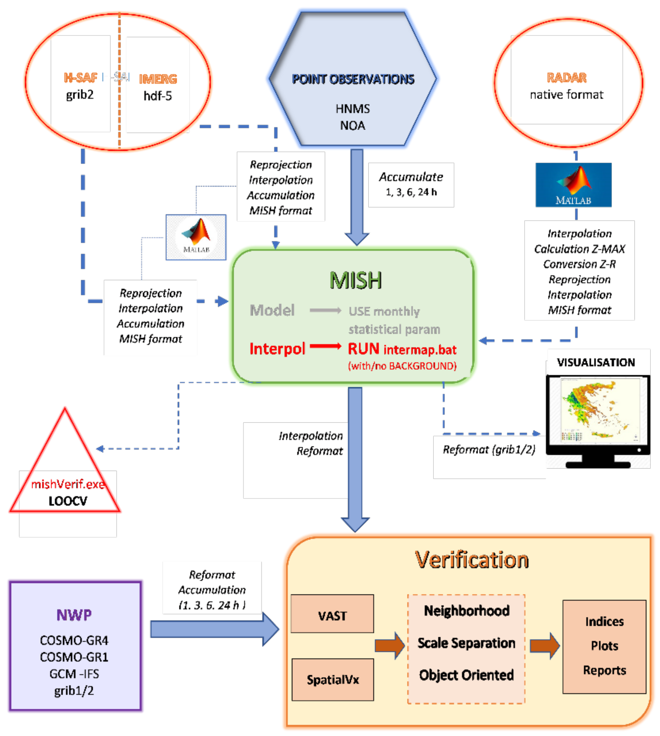
The proposed Integrated Forecast Evaluation System (IFES) aims to address the primary conditions for the application of sophisticated spatial verification methods, specifically the acquisition of gridded observations for the most realistic representation of the true state of the atmosphere, but also the targeted application of certain verification methods to better highlight the characteristics of predicted precipitation fields. The system is adapted to the needs of the Greek territory, providing sufficient information concerning the skill of high-resolution numerical models in areas with intense relief and frequently insufficient sources of in situ observations. Specifically, the methodology applied to generate statistics on a daily basis includes the components and flow shown in detail in
Figure 1, and consists of the following steps: (1) gathering ground observations from all available ground based networks and format adjustment for input to MISH interpolation module; (2) aggregation of available radar data, application of filters/adaptations (e.g., radial velocity filter, Z–R conversion) and adjustment as input to MISH; (3) H-SAF data aggregation and adaptation (reprojection/interpolation in cartesian grid) and adjustment as input to MISH; (4) MISH interpolation module execution with appropriate customization of input data from the modeling module and use of surface observations with the choice of using background fields (radar and/or satellite data); (5) MISH output conversion to verification software requirements and adaptation to the resolution of the NWP model to be evaluated; (6) application of verification software, including VAST for neighborhood methods and SpatialVx for field displacement or methods; and finally (7) production of statistical indices, graphs and analysis of results.
4. Application of IFES
Following the development of the IFES components, the evaluation procedure was applied to several weather systems accompanied by precipitation over Greece, one of which is presented in this paper. The aim is to demonstrate the potential value of the system, to determine the optimal approach in relation to the use (or not) of background fields in the creation of gridded observations, as well as to highlight the information on the quality of the numerical forecasts provided by the different verification methods.
In this study, the precipitation forecasts evaluated were produced by the COSMO model used by the Hellenic National Meteorological Service (HNMS). COSMO is a non-hydrostatic model developed by the COSMO (Consortium for Small scale Modeling) Consortium to provide high spatial resolution forecasts as well as a flexible tool for a variety of research applications. There are two versions of the model: COSMOGR1 with a horizontal resolution of 0.01° (~1 km) capable of resolving convection and COSMOGR4 with a resolution of 0.04° (~4 km), which is a parameterized convection scale that is also used to initialize COSMOGR1. Improvements in microphysical schemes in the convection-scale COSMO model have enabled it to provide improved accuracy with respect to the location, timing and severity of deep convection resulting in improved precipitation forecasts, in particular during the summer period compared to NWP models with lower resolution that rely upon parameterization of deep convection [
33]. The performance of the model’s main output, including temperature, precipitation, wind, cloud, etc., is evaluated on a daily basis at HNMS to assess the reliability of the models but also to highlight systematic errors [
28]. In the present study, the proposed evaluation framework (IFES) focuses on the systematic evaluation of the two versions of the model, specifically in areas with strong relief using methods that are easy to use and computable on an operational basis. On the other hand, the specific characteristics of the precipitation field can be analyzed in order to demonstrate, in an objective way, the superiority of convection resolving models to produce a more realistic representation of precipitation.
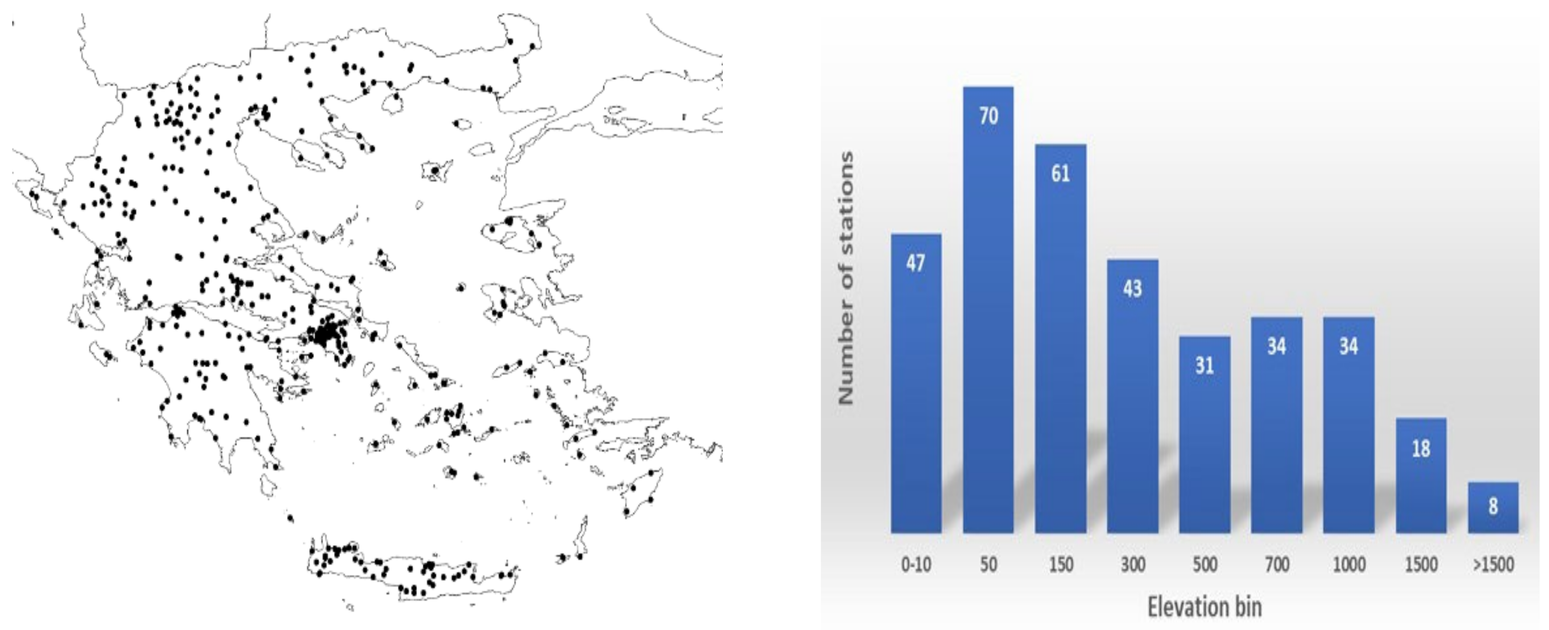
As a first step, gridded observations were created for the accumulated precipitation. Next, background observation information was added from satellite and radar estimated precipitation fields and the impact on the interpolated observation field for the specific weather situation was evaluated. Finally, the NWP forecasts were evaluated with two different spatial verification methods, each highlighting different qualitative characteristics of the numerical models in terms of precipitation predictability. For the specific application, surface observations were obtained from HNMS’ network of meteorological stations as well as the network of the National Observatory of Athens (NOA). Many of the stations are located at medium to high altitudes (~70 stations above 1000 m), which is critical for spatial representation of rain in areas with intense relief. The geographical distribution of the stations and the histogram of the range of their altitudes are given in
Figure 2.
4.1. Synoptic Situation
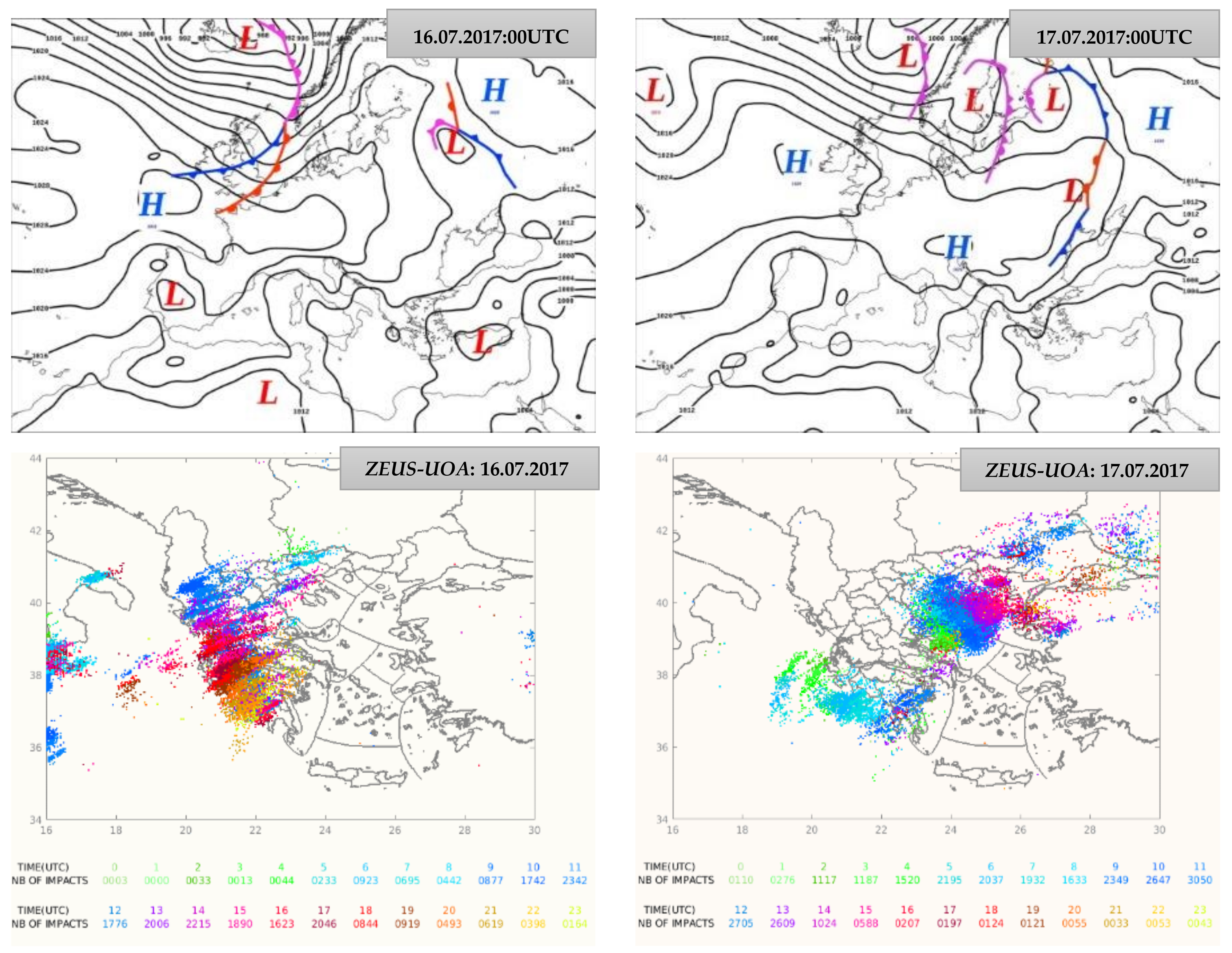
A rather unusual meteorological event, with regard to both the season and the duration, extent and intensity of the phenomena, took place over Greece on 16 and 17 July 2017. The system was characterized by intense phenomena (rain, hail), rapid accumulation of precipitation, extended duration of the phenomena, strong electrical activity and winds whose surface gusts exceeded 40 knots (8–9 B). The surface analysis 16 July 2017/00UTC (left) and 17 July 2017/00UTC (right) is given in
Figure 3. Low pressure of around 1004 hPa prevails in the southeastern Mediterranean while in the area of the southern Ionian Sea a closed barometric low (1012 hPa) has developed. On 17 July 2017 the cyclonic circulation over the southern Ionian persists, while the Azores anticyclone has extended over Eastern Europe and the northern Balkans and a strong convergence zone is evident above the eastern mainland of Greece and part of northern Aegean Sea. The combination of high pressure (1020 hPa) over the northern Balkans with low pressure over Turkey (1006 hPa) results in strong northeasterly flow over the northern Aegean.
4.2. Development of Gridded Observation with/without Background
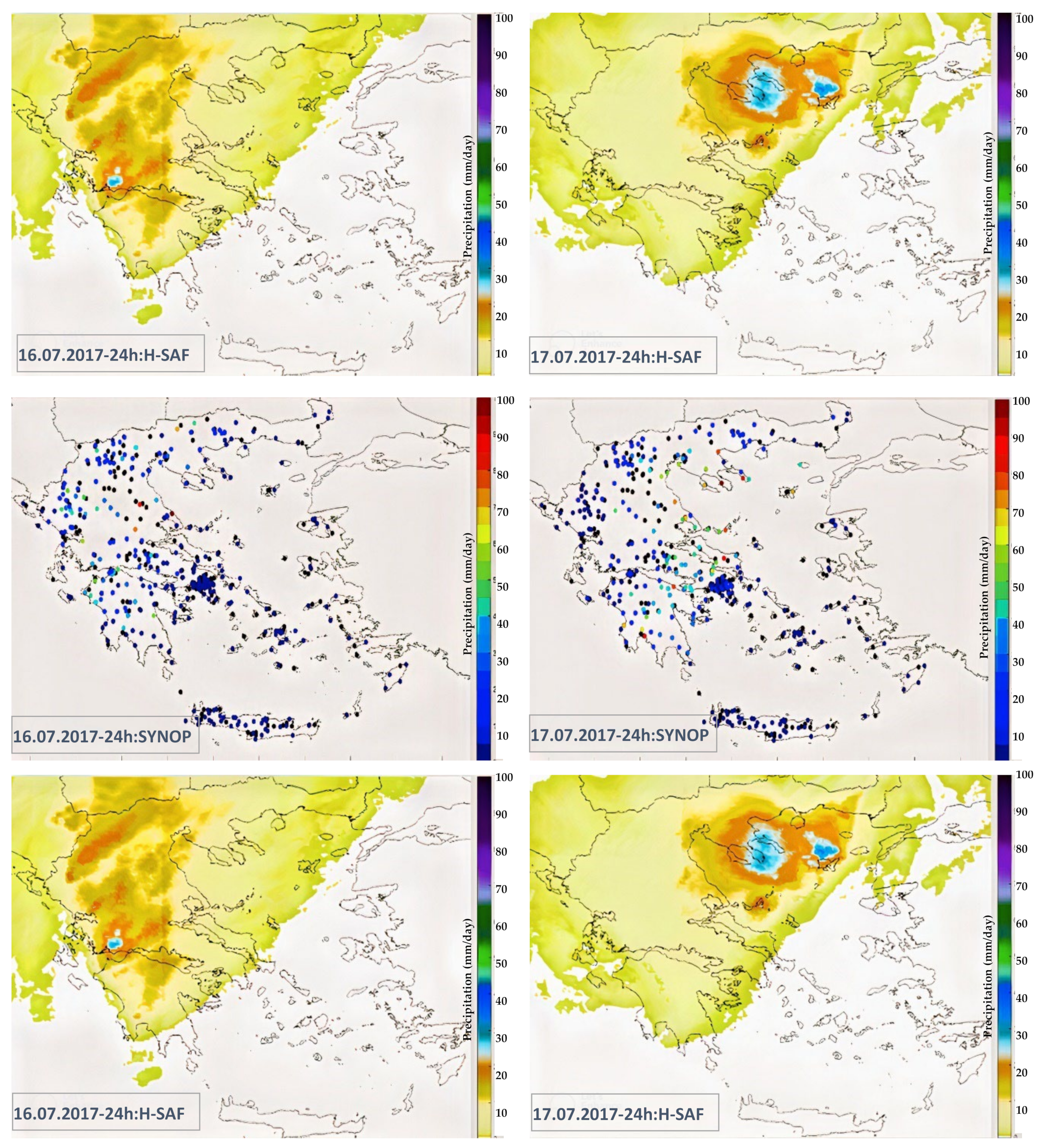
Surface observations were used to generate gridded observations for the cumulative 24-h precipitation. Significant amounts of precipitation fell on 16 July in the west and central mainland of Greece, while on 17 July even higher amounts (>70 mm/24 h) were recorded in the eastern as well as parts of the northern mainland (
Figure 4). Rainfall estimates retrieved from H-SAF product H05 are also shown in
Figure 4. The color scale indicates areas where differences exist between the surface observations and the H-SAF data, the latter being significantly lower. Previous research [
34] has identified the tendency of precipitation product H05 to underestimate the amount of rain in cases of severe weather. It should be noted however that the satellite product H05 allows precipitation estimates over the sea, providing a comparative advantage in spatial coverage, especially around Greece’s many islands.
Precipitation estimates were inserted into a latitude-constant latitude grid with a spatial pitch of 0.03 degrees. The interpolation methodology was then applied to generate the gridded observations with the MISH software as part of IFES framework. The first step in generating the interpolated precipitation field is to perform the modeling process with the MISH software. Although the modeling system is based on monthly climatological data, daily or even shorter rainfall intervals can be interpolated using the correlations resulting from the modeling process. For the case being analyzed, the correlations between rainfall and geophysical parameters from the month of July were used since they had the best correlation coefficient (R): 0.778 [
4].
The gridded fields with spatial resolution of 0.00833° resulting from the MISH interpolation are shown for both days with ground observations only and with an H-SAF background (
Figure 5). The areas that received the highest precipitation amounts are the same as those in
Figure 4, but with more detailed structure and some local maxima differences between the two different approaches. It should be noted that the marine areas have been removed from the final precipitation field since the interpolation methodology is based on climatological data and correlations with geophysical parameters that do not include bodies of water. The results show that when the background field is used, the overall structure of the rainfall exhibits differences compared to that created by MISH without the additional information from the satellite data. The relative weight the MISH software gives to the background information is less than that given to the surface observations, while the weight coefficient at each point depends on the extent that the surface observation field differs from the background. Over the marine areas where there are no observations, nor available correlations from MISH modeling, the satellite data take precedence.
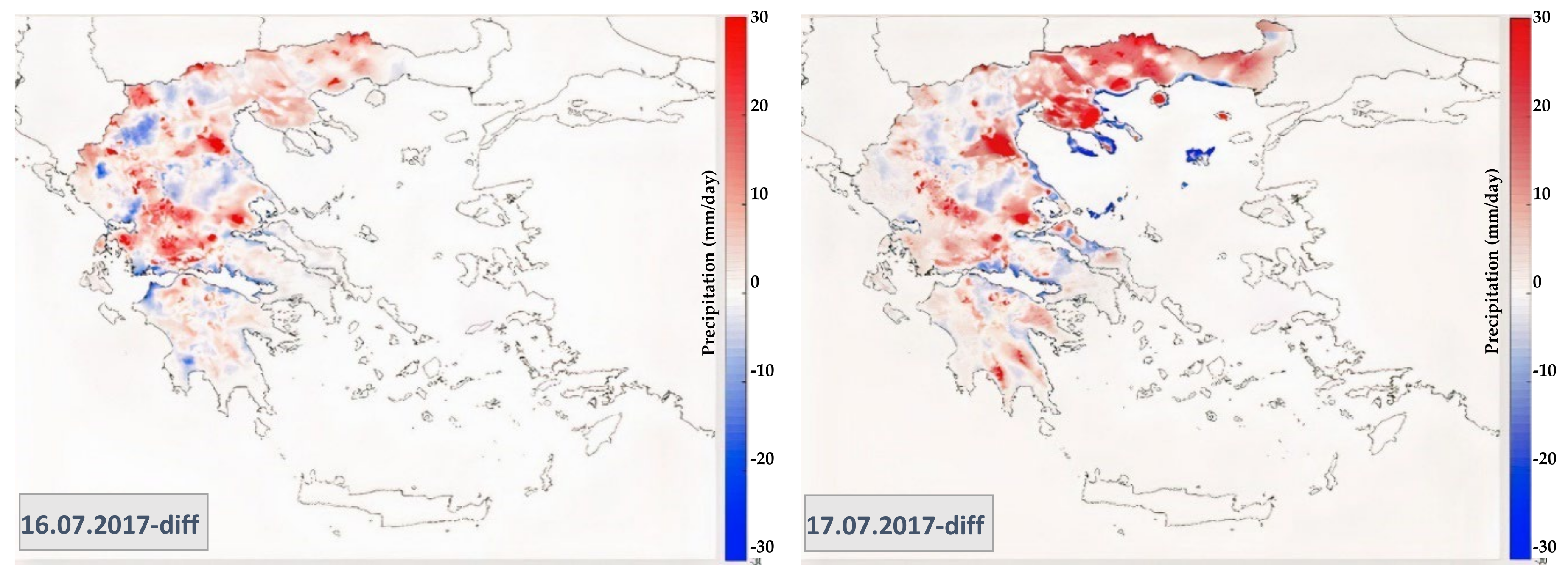
The representation of the field differences of the interpolated observations extracted from MISH highlights the basic differences between the derived fields (
Figure 6). Specifically, the field of differences was created by subtracting the value created using background information from that created without. Positive deviations (red) are located mainly in mountainous areas, highlighting the effect of orography and of its ability to amplify precipitation as altitude increases. The use of the background field appears to significantly smooth out the maximums and produces a gradation of the rain around the mountainous areas. In contrast, negative deviations (blue) are evident around areas closer to sea level, especially on 17 July when high precipitation amounts were measured over Chalkidiki (northern peninsula) and in the wider area of the Western Thracian Sea. Since values in these areas were mainly derived from the H-SAF data, this resulted in an increase in rainfall values due to the aforementioned tendency for overestimation.
4.3. Statistical Evaluation of Interpolation Method
In order to objectively assess the error associated with the application of this methodology in the production of daily interpolated observed values, a statistical evaluation was performed. A code was developed that allowed the application of the Cross Validation Leave-One-Out (LOOCV) technique [
35]. The MISH interpolation module was applied N times (N = number of stations) with all data except one point (one surface station measurement) and an estimate is made for this point. In the specific case study, the number of stations used and therefore the number of repetitions was 321. LOOCV is essentially an estimate of the general performance of the MISH model based on N-1 data samples. Once the estimate of the precipitation value for the removed station has been calculated, statistical indices are calculated in order to estimate the deviation from the actual observed value. This evaluation process was performed with or without the use of the background field (H-SAF estimates).
The indices used are the Normalized Mean Error (
NME) [
36]:
and the Normalized Root Mean Square Error (
NRMSE) [
37]:
where
is the precipitation value estimated by the MISH model at the point of observation that was subtracted from the interpolation procedure,
the value of the observation at that point, and
the average value of the observations. The NRMSE was chosen as an index for evaluating the performance of the method, and is included in the IFES, because it allows for the examination of the average error between samples of different scale (range of values) and even different units. The NME also highlights the trend of deviation from the observed value (negative value/underestimation, positive value/overestimation) as a percentage of the normalized difference, making it possible to compare values between samples with different distributions of the observed precipitation values.
These statistical values were calculated for each forecast day as well as for the two types of gridded fields, with or without background field. The mean values of NME (%) and NRMSE are shown in
Figure 7. From the results, it appears that the interpolation approach of MISH has the tendency, as an average of all repetitions at N-1 stations, to underestimate the amount of 24-h precipitation in all cases (negative NME) with higher error values on 16 July 2017, when the NME reaches the value −16%. It should be noted that the average NME for the 321 observations was −9.2% on 16 July and 14.6% on 17 July. The use of background fields for both days of the event slightly reduces the range of the negative deviation while maintaining the tendency to underestimate. Furthermore, the NRMSE values give an indication of the average normalized deviation with respect to the mean of observations and ranges between 1–1.7 mm/24 h (the values of the non-normalized RMSE are 14–15 mm/24 h). The NRMSE results indicate that the use of background information reduced, but not significantly, the average error although, as mentioned above, its use had a very important role in places where there were no observations and especially near or over the sea, consequently improving the overall structure of the precipitation field in the domain of interest, even though this is not reflected in the statistical indices.
4.4. Forecast Verification
The initial motivation to create gridded observations was to be able to apply spatial statistical methods of objective verification, in order to better understand the strengths and weaknesses of high-resolution precipitation forecasts over the complex terrain of Greece. The gridded data created as described previously was used to apply the final module of IFES to the precipitation forecasts for the selected weather event. Simulations with the numerical models COSMOGR4 and COSMOGR1 were used and the forecasted 24 h accumulated precipitation amounts of 16 July 2017 runs initiated at 00UTC, are given in
Figure 8. During the application of verification approaches in IFES, necessary adjustments to the observed fields are applied in order for the spatial analysis to be at exactly the same scale with that of the forecasted field. COSMOGR4 is initialized from the IFS (ECMWF) global model while COSMOGR1 is nested and takes its initial and boundary conditions from COSMOGR4.
4.4.1. Fuzzy Approach
Neighborhood verification is based on the principle of extending the field of view to nearby data points (“neighbors”) in space, creating a spatial window around the forecast and observation points. During the application of the method, a number of spatial indices and averaging techniques are generated by the VAST software (COSMO,
www.cosmo-model.org, accessed on 10 June 2022), but for the operational verification requirements in the proposed IFES system, only the most representative for the performance of the NWP forecasts are presented here. Considering the relative performance of the two versions of COSMO, the decision model (criterion for a successful event within a window for each rainfall threshold) used to determine a successful forecast was not strict, which is a determining factor of the methods that will be used to evaluate the performance. The values of the statistical indices (scores) are presented as intensity scale diagrams, where the intensity threshold and the spatial scale increase along the x and y axes, respectively, and the color shade gives an indication of the score value.
It is possible to evaluate the performance of the model without focusing on the absolute value of each color window but rather by examining the color intensity, scales and thresholds. A selection of the evaluation graphs generated by IFES for the COSMOGR4 and COSMOGR1 forecasts is presented in
Figure 9. The spatial windows (y axis) are different for the two models since the smoothing is based on multiples of the initial spatial resolution of the model and takes values from 4–68 km for COSMOGR4 and 1–17 km for COSMOGR1 while the precipitation thresholds (x axis) range from 0.1–10 mm/24 h.
The following conclusions can be drawn from the statistical indicators: The FSS (first row, column 1–2), which essentially gives the frequency fraction of the occurrence of a rainfall threshold in the forecast in relation to that of the observation field, has values higher than 0.8 (with an optimal value of 1) for the various spatial windows without the spatial smoothing for COSMOGR4 for the threshold higher than 1 mm/24 h while for COSMOGR1 for the threshold higher than 2.5 mm/24 h. Comparison between models shows high values of FSS for different spatial scales, specifically for windows larger than 12 km for COSMOGR4 and larger than 3 km for COSMOGR1 and for varying thresholds.
Two statistical indices (BIAS and POD) were calculated using the Upscaling spatial filter that applies the average value of rainfall to constantly expanding spatial windows. The BIAS (first row, column 3–4) for both models highlight an underestimation of rainfall amounts (BIAS < 1) for all thresholds and spatial scales for COSMOGR4 but slightly less so for COSMOGR1. The Probability of Detection (POD) (second row, column 1–2) values improve almost linearly for COSMOGR4 with increasing threshold and spatial scale, while the probability of a successful forecast of a rainfall threshold is very small, especially for larger amounts of rain, for COSMOGR1 at spatial scales at or below 9 km.
The same linear dependence of the POD on the amount of rain and spatial window is indicated on the summary POD plot (third row, column 3–4) in
Figure 9. The improved performance of the COSMOGR4 model confirms the hypothesis that lower resolution models have better POD due to their ability to represent more spatially diffused precipitation, which leads to more statistically successful forecasts.
Following the application of the “Anywhere in the Window” filter, which is the least stringent decision model used in this study, the FAR index was calculated (second row, column 3–4). Although both simulations show low FAR values due to erroneous precipitation warnings, COSMOGR1 clearly outperforms its lower resolution counterpart, especially for thresholds >4 mm/24 h for all spatial windows.
The magnitude of average error at all scales is given by the value of the area_RMSE index (third row, column 1–2), which represents a more traditional point verification approach. The index range for both models is 20–23 mm/24 h, at which values for COSMOGR1 are lower in comparison to COSMOGR4 at the same spatial scales.
4.4.2. Object Oriented Approach
The SAL method is applied for the forecasts of both the COSMOGR4 and COSMOGR1 models in comparison with the grid observations that emerged with the MISH software for each 24-h forecast (16–17 July 2017). Application of this method requires optimization of all the parameterizations included in the calculation routines. It is not required that the objects of the observation and the forecast fields have a one-to-one correlation. Objects are identified separately through the Feature Finder routine. The main issues to be considered are: (a) matching the size of the application area for observations and forecasts and it is recommended not to be too large as components from different precipitation systems may overlap, (b) the precipitation accumulation interval should be large enough to avoid noise in object identification. Regarding its configuration, the most important element is the selection of a threshold for object identification, which can be critical if fields contain objects with different local maxima. The are many possibilities for defining a threshold R reported in the literature, but for the proposed evaluation system a fraction of the 95th percentile of field values (separately for forecast and observation) exceeding 0.1 mm was applied as a threshold. A coefficient of 1/15 was used [
31] which is an approach influenced by outliers.
Another important parameterization is the smoothpar option, in which the value at each point of the grid is replaced by the average value over a disk with a radius of several grid points given by the parameter. The collected data is then bounded by thresholds creating a binary mask, therefore affecting the boundaries of objects which are smoothed by filtering out small-scale noise. The choice of smoothing radius is not straightforward [
38] and is dependent upon the size of the grid. Thus, the same smoothpar can lead to minimal smoothing when applied to a 1 km grid but quite significant results for coarser grids, leading, for example, to the creation of “bridges” between different objects located close to one another. For this study, a smoothing factor of 2 was used. The omission of small objects defined via the min.size option (min.size = c(n_min_obs, nmin_fcs)) of FeatureFinder is also an important parameter that defines the coherent objects, omitting those where a threshold depending on the number of points it is derived from (n.min) is exceeded. During the application of the SAL method for the evaluation of the forecasts, the objects can be visualized following the application of the Feature Finder function. In order to determine the optimal definition of the various parameters for the proposed evaluation system, average values have been selected.
For the weather episode of 16–17 July 2017, the SAL method was applied and the parameters S, A, and L were calculated for each model for each forecast day. The SAL component values are depicted in the diagrams in
Figure 10. A perfect forecast is characterized by a value of zero for all three SAL components. The taSAL = (|S| + |A| + |L|) index proposed by Lawson and Gallus [
39] (as an objective performance indicator) is also given in the same diagram. For both models, the forecast skill for 24 h precipitation was higher for the period of 16 July without significant differences in the performance between the two models. Quantitative evaluation based on component A produced satisfactory results, with COSMOGR4 producing a slightly better estimation while COSMOGR1 slightly overestimated rainfall on 16 July. Analyzing the index S for the shape and size of the rain objects, the objects forecast for 16 July were bigger and wider (flatter) for both models, while the exact was opposite for 17 July. Regarding the L index and the relative location of the objects, the COSMOGR1 model tended to provide more successful forecasts regarding the location of the rain system (relatively smaller values of L) for both days.
5. Conclusions
Spatial resolution of NWP models is constantly increasing as computing power continues to expand, leading to the expectation that this will lead to improved forecasts of local weather conditions, in particular of precipitation. The spatial patterns of high-resolution precipitation forecasts are rendered with very realistic structures since models can accurately reproduce dynamic and thermodynamic atmospheric processes. The corresponding field of observed values is usually, however, less spatially detailed, making direct comparison at the point-of-observation level a challenge for the systematic evaluation of forecasts.
The focus of this work was the development of a methodology and an integrated forecast evaluation system that would more accurately assess the ability of high-definition model products to produce a precipitation forecast by using new spatial verification techniques. A particular emphasis was placed on the creation of reliable gridded fields of observations through the appropriate adaptation of a methodology based on the use of climate data and correlation (multiple regression) of such time series with geophysical parameters in the course of applying interpolation schemes. The application of spatial verification methods requires the creation of high-resolution gridded precipitation observations. The study focused on the Greek territory, which represents a unique case due to the lack of density and complete geographical coverage of the networks of surface observations, the limited possibility of continuous and uninterrupted coverage by radar networks for the quantitative estimation of precipitation in high spatial resolution, as well as its complex relief with large water surfaces as well as high gradient topography and the extensive number of islands.
Based on previous experience with other meteorological parameters, the MISH method, which is a meteorological interpolation system designed to use all meteorological, climatological and basic information of the geophysical environment of the area of interest, was applied for the production of gridded observations. The modelling of a long climatological time series produced correlations (optimal parameters per month) with the topographic characteristics for a grid with a resolution of 0.0083333°. This was followed by a process of interpolating surface observations as part of the IFES, using the results of the modeling and the optimal statistical parameters of the corresponding month, as well as using additional background fields from precipitation estimates from satellite and/or radar (depending on their availability as appropriate).
A comprehensive application of the IFES was presented in the context of an evaluation of the forecasts of a highly convective weather event. The objective was to differentiate the performance of the two operational versions of COSMO-GR model at different resolutions. The application highlighted the importance of using high spatial resolution backgrounds to improve observed field realism, mainly over geographic areas with limited or non-existent ground station coverage. The evaluation of the precipitation forecasts was accomplished by applying two spatial methods belonging to the categories of filtering and object identification, defining a flexible and computationally efficient framework. The analysis highlighted both the qualitative characteristics of the predictions of the two models as well as the multitude of possibilities arising from the parameterization of the evaluation procedure.
The proposed verification system for precipitation forecasts addresses the requirements of an operational system oriented to meet the needs of a variety of users. The system is based on satisfying the primary prerequisite for the application of innovative spatial verification methods, which is the creation of gridded observations for an improved representation of the true state of the atmosphere, but also the targeted application of certain verification methods to better highlight the characteristics of the predicted precipitation fields. The system has been adapted to the specific needs of the Greek territory, namely to provide sufficient information for the skill of a very high-resolution numerical model in areas with challenging topography.
Author Contributions
Conceptualization, F.G., H.F. and P.L.; methodology, F.G.; software, F.G. and I.S.; validation, F.G.; formal analysis, F.G.; investigation, F.G.; resources, F.G. and I.S.; data curation, F.G. and I.S.; writing—original draft preparation, F.G.; writing—review and editing, H.F. and P.L.; visualization, I.S.; supervision, H.F. All authors have read and agreed to the published version of the manuscript.
Funding
This research received no external funding and the APC was funded by COSMO consortium.
Institutional Review Board Statement
Not applicable.
Informed Consent Statement
Not applicable.
Acknowledgments
The authors would like to express their sincere gratitude to HNMS and NOA for the kind provision of precipitation data from their respective meteorological station networks.
Conflicts of Interest
The authors declare no conflict of interest.
References
- Rossa, A.; Nurmi, P.; Ebert, E. Overview of Methods for the Verification of Quantitative Precipitation Forecasts. In Precipitation: Advances in Measurement, Estimation and Prediction; Michaelides, S., Ed.; Springer: Berlin/Heidelberg, Germany, 2008. [Google Scholar] [CrossRef]
- Casati, B.; Wilson, L.J.; Stephenson, D.B.; Nurmi, P.; Ghelli, A.; Pocernich, M.; Damrath, U.; Ebert, E.E.; Brown, B.G.; Mason, S. Forecast verification: Currentstatus and future directions. Meteorol. Appl. 2008, 15, 3–18. [Google Scholar] [CrossRef]
- Flocas, A. Courses of Meteorology and Climatology; Zitis, Ed.; Firenze University Press: Thessaloniki, Greece, 1994. (In Greek) [Google Scholar]
- Gofa, F.; Mamara, A.; Anadranistakis, M.; Flocas, H. Developing Gridded Climate Data Sets of Precipitation for Greece Based on Homogenized Time Series. Climate 2019, 7, 68. [Google Scholar] [CrossRef] [Green Version]
- Levizzani, V.; Kidd, C.; Aonashi, K.; Bennartz, R.; Ferraro, R.R.; Huffman, G.J.; Roca, R.; Turk, F.J.; Wang, N.-Y. The activities of the International Precipitation Working Group. Q. J. R. Meteorol. Soc. 2018, 144, 3–15. [Google Scholar] [CrossRef] [PubMed] [Green Version]
- Verworn, A.; Haberlandt, U. Spatial interpolation of hourly rainfall—Effect of additional information, variogram inference and storm properties. Hydrol. Earth Syst. Sci. 2011, 15, 569–584. [Google Scholar] [CrossRef] [Green Version]
- Burrough, P.A.; McDonnell, R.A. Principles of Geographical Information Systems; Oxford University Press: Oxford, UK, 1998. [Google Scholar]
- Wagner, P.D.; Fiener, P.; Wilken, F.; Kumar, S.; Schneider, K. Comparison and evaluation of spatial interpolation schemes for daily rainfall in data scarce regions. J. Hydrol. 2012, 464–465, 388–400. [Google Scholar] [CrossRef]
- Daly, C.; Halbleib, M.; Smith, J.I.; Gibson, W.P.; Doggett, M.K.; Taylor, G.H.; Curtis, J.; Pasteris, P.A. Physiographically-sensitive mapping of temperature and precipitation across the conterminous United States. Int. J. Climatol. 2008, 28, 2031–2064. [Google Scholar] [CrossRef]
- Sevruk, B. Regional Dependency of Precipitation-Altitude Relationship in the Swiss Alps. Clim. Change 1997, 36, 355–369. [Google Scholar] [CrossRef]
- Sinclair, M.R.; Wratt, D.S.; Henderson, R.D.; Gray, W.R. Factors affecting the distribution and spillover of precipitation in the Southern Alps of New Zealand—A case study. J. Appl. Meteorol. 1997, 36, 428–442. [Google Scholar] [CrossRef]
- Chow, V.T.; Maidment, D.R.; Mays, L.W. Applied Hydrology; McGraw Hill: New York, NY, USA, 1998. [Google Scholar]
- Daly, C. Variable Influence of Terrain on Precipitation Patterns: Delineation and Use of Effective Terrain Height in PRISM; Oregon State University: Corvallis, OR, USA, 2002. [Google Scholar]
- Feidas, H.; Karagiannidis, A.; Keppas, S.; Vaitis, M.; Kontos, T.; Zanis, P.; Melas, D.; Anadranistakis, E. Modelling and mapping temperature and precipitation climate data in Greece using topographical and geographical parameters. Theor. Appl. Climatol. 2013, 118, 133–146. [Google Scholar] [CrossRef]
- Szentimrey, T.; Bihari, Z. Manual of interpolation software MISHv1.03. Hung. Meteorol. Serv. 2014, 59. [Google Scholar]
- Szentimrey, T.; Bihari, Z.; Szalai, S. Comparison of geostatistical and meteorological interpolation methods (what is what?). In Spatial Interpolation for Climate Data: The Use of GIS in Climatology and Meteorology; Wiley: Hoboken, NJ, USA; International Society for Technology in Education: London, UK, 2007; pp. 45–56. [Google Scholar]
- Mamara, A.; Anadranistakis, M.; Argiriou, A.A.; Szentimrey, T.; Kovacs, T.; Bezes, A.; Bihari, Z. High Resolution Air Temperature Climatology for Greece for the Period 1971–2000. Meteorol. Appl. 2017, 24, 191–205. [Google Scholar] [CrossRef] [Green Version]
- Bénichou, P.; Le Breton, O. Aurelhy: Une méthode d’analyse utilisant le relief pour les bésoins de l’hydrométéorologie. In Deuxièmes Journées Hydrologiques de L’orstom à Montpellier; Office of Scientific and Technical Research Overseas: Marseille, France, 1989; pp. 299–304. [Google Scholar]
- Mugnai, A.; Smith, E.A.; Tripoli, G.J.; Bizzarri, B.; Casella, D.; Dietrich, S.; Di Paola, F.; Panegrossi, G.; Sanò, P. CDRD and PNPR Satellite Passive Microwave Precipitation Retrieval Algorithms: EuroTRMM/EURAINSAT Origins and H-SAF Operations. Nat. Hazards Earth Syst. Sci. 2013, 13, 887–912. [Google Scholar] [CrossRef] [Green Version]
- Puca, S.; Porcù, F.; Rinollo, A.; Vulpiani, G.; Baguis, P.; Balabanova, S.; Campione, E.; Ertürk, A.; Gabellani, S.; Iwanski, R.; et al. The validation service of the hydrological SAF geostationary and polar satellite precipitation products. Nat. Hazards Earth Syst. Sci. 2014, 14, 871–889. [Google Scholar] [CrossRef]
- Porcù, F.; Milani, M.; Petracca, M. On the uncertainties in validating satellite instantaneous rainfall estimates with raingauge operational network. Atmos. Res. 2014, 144, 73–81. [Google Scholar] [CrossRef]
- Cassola, F.; Ferrari, F.; Mazzino, A. Numerical simulations of Mediterranean heavy precipitation events with the WRF model: Analysis of the sensitivity to resolution and microphysics parameterization schemes. Atmos. Res. 2015, 164, 210–225. [Google Scholar] [CrossRef]
- Wulfmeyer, V.; Behrendt, A.; Kottmeier, C.; Corsmeier, U.; Barthlott, C.; Craig, G.C.; Hagen, M.; Althausen, D.; Aoshima, F.; Arpagaus, M.; et al. The Convective and Orographically-induced Precipitation Study (COPS): The scientific strategy, the field phase, and research highlights. Q. J. R. Meteorol. Soc. 2011, 137, 3–30. [Google Scholar] [CrossRef]
- Brown, B.G.; Gilleland, E.; Ebert, E.E. Forecasts of Spatial Fields. Forecast Verification: A Practitioner’s Guide in Atmospheric Science, 2nd ed.; Jolliffe, I.T., Stephenson, D.B., Eds.; Wiley: Hoboken, NJ, USA, 2012; 274p. [Google Scholar]
- Gilleland, E.; David, A.; Ahijevych, D.; Brown, B.G.; Ebert, E.E. Verifying Forecasts Spatially. Bull. Am. Meteorol. Soc. 2010, 91, 1365–1373. [Google Scholar] [CrossRef] [Green Version]
- Gofa, F.; Boucouvala, D.; Louka, P.; Flocas, H.A. Spatial verification approaches as a tool to evaluate the performance of high resolution precipitation forecasts. Atmos. Res. 2017, 208, 78–87. [Google Scholar] [CrossRef]
- Gilleland, E.; Ahijevych, D.; Brown, B.G.; Casati, B.; Ebert, E.E. Intercomparison of Spatial Forecast Verification Methods. Weather Forecast. 2009, 24, 1416–1430. [Google Scholar] [CrossRef]
- Gofa, F.; Pytharoulis, I.; Andreadis, T.; Papageorgiou, I.; Fragkouli, P.; Louka, P.; Avgoustoglou, E.; Tyrli, V. Evaluation of the Operational Numerical Weather Forecasts of the Hellenic National Meteorological Service. In Proceedings of the 9th COMECAP Conference of Meteorology, Thessaloniki, Greece, 28–31 May 2008; pp. 51–58. [Google Scholar]
- Fowler, T.L.; Jensen, T.; Tollerud, E.I.; Halley Gotway, J.; Oldenburg, P.; Bullock, R. New Model Evaluation Tools (MET) software capabilities for QPF verification. Preprints. In Proceedings of the 3rd International Conference on QPE/QPF and Hydrology, Nanjing, China, 18–22 October 2010; WMO/World Weather Research Programme: Geneva, Switzerland, 2010. [Google Scholar]
- R Development Core Team. R: A Language and Environment for Statistical Computing; R Foundation for Statistical Computing: Vienna, Austria, 2011; ISBN 3-900051-07-0. Available online: http://www.R-project.org (accessed on 10 June 2022).
- Wernli, H.; Hofmann, C.; Zimmer, M. Spatial Forecast Verification Methods Intercomparison Project: Application of the SAL Technique. Weather Forecast. 2009, 24, 1472–1484. [Google Scholar] [CrossRef]
- Wernli, H.; Paulat, M.; Hagen, M.; Frei, C. SAL—A novel quality measure for the verification of quantitative precipitation forecasts. Mon. Weather. Rev. 2008, 136, 4470–4487. [Google Scholar] [CrossRef] [Green Version]
- Baldauf, M.; Seifert, A.; Förstner, J.; Majewski, D.; Raschendorfer, M.; Reinhardt, T. Operational convective-scale numerical weather prediction with the COSMO model: Description and sensitivities. Mon. Weather. Rev. 2011, 139, 3887–3905. [Google Scholar] [CrossRef]
- Feidas, H.; Porcù, F.; Puca, S.; Rinollo, A.; Lagouvardos, C.; Kotroni, V. Validation of the H-SAF precipitation product H03 over Greece using rain gauge data. Theor. Appl. Climatol. 2018, 131, 377–398. [Google Scholar] [CrossRef]
- Arlot, S.; Celisse, A. A survey of cross-validation procedures for model selection. Stat. Surv. 2010, 4, 40–79. [Google Scholar] [CrossRef]
- Gustafson, W.I., Jr.; Yu, S. Generalized approach for using unbiased symmetric metrics with negative values: Normalized mean bias factor and normalized mean absolute error factor. Atmos. Sci. Lett. 2012, 13, 262–267. [Google Scholar] [CrossRef]
- Poli, A.A.; Cirillo, M.C. On the use of the normalized mean square error in evaluating dispersion model performance. Atmos. Environ. 1993, 27, 2427–2434. [Google Scholar] [CrossRef]
- Weniger, M.; Friederichs, P. Using the SAL Technique for Spatial Verification of Cloud Processes: A Sensitivity Analysis. J. Appl. Meteorol. Climatol. 2016, 55, 2091–2108. [Google Scholar] [CrossRef]
- Lawson, J.R.; Gallus, W.A. Adapting the SAL method to evaluate reflectivity forecasts of summer precipitation in the central United States. Atmos. Sci. Lett. 2016, 17, 524–530. [Google Scholar] [CrossRef]
| Publisher’s Note: MDPI stays neutral with regard to jurisdictional claims in published maps and institutional affiliations. |
© 2022 by the authors. Licensee MDPI, Basel, Switzerland. This article is an open access article distributed under the terms and conditions of the Creative Commons Attribution (CC BY) license (https://creativecommons.org/licenses/by/4.0/).


