Article

Comparison of East Asian Summer Monsoon Simulation between an Atmospheric Model and a Coupled Model: An Example from CAS-ESM

1
Key Laboratory for Meteorological Disaster Monitoring and Early Warning and Risk Management of Characteristic Agriculture in Arid Regions, China Meteorological Administration, Yinchuan 750002, China
2
International Center for Climate and Environment Sciences, Institute of Atmospheric Physics, Chinese Academy of Sciences, Beijing 100029, China
3
Ningxia Hui Autonomous Region Climate Center, Yinchuan 750002, China
*
Author to whom correspondence should be addressed.
Atmosphere 2022, 13(7), 998; https://doi.org/10.3390/atmos13070998
Submission received: 17 May 2022 / Revised: 15 June 2022 / Accepted: 16 June 2022 / Published: 21 June 2022
(This article belongs to the Special Issue Coupled Climate System Modeling)

Abstract

:
In this study, the Chinese Academy of Sciences’ Earth System Model Version 2 (CAS-ESM2) and its atmospheric component were evaluated for the ability to simulate the East Asian summer monsoon (EASM), in terms of climatology and composites in El Niño decaying years (EN) and La Niña years (LN). The results show that the model can realistically simulate the El Niño Southern Oscillation (ENSO) annual cycle, the interannual variation, the evolution process, and the prerequisites of ENSO, but the trend of developing and decaying is faster than that of the observations. With regard to the climatological mean state in the EASM, the coupled model run can largely improve the precipitation and 850 hPa wind simulated in the atmospheric model. Moreover, the coupled run can also reduce the mid-latitude bias in the atmospheric model simulation. Composite methods were then adopted to examine performance in different phases of the ENSO, from a mature winter to a decaying summer. The atmospheric model can well reproduce the Western North Pacific Anomalous Anticyclone (WNPAC)/Western North Pacific Anomalous Cyclone (WNPC) during EN/LN well, but the westerly/easterly anomalies and the associated precipitation anomalies over the equatorial Central Eastern Pacific are somewhat overestimated. Compared with the atmospheric model, these anomalies are all underestimated in the coupled model, which may be related to the ENSO-related SST bias appearing in the Eastern Indian Ocean. Due to the ENSO and ITCZ bias in the historical simulations, the simulated ENSO-related SST and the precipitation anomaly are too equator-trapped in comparison with the observations, and the cold tongue overly extends westward. This limits the ability of the model to simulate ENSO-related EASM variability. For the subseasonal simulations, though atmospheric model simulations can reproduce the westward extension of the Western Pacific subtropic high (WPSH) in EN decaying summers, the eastward retreat of the WPSH in LN is weak. The historical simulations show limited improvement, indicating that the subseasonal variation in the EASM is still a considerable challenge for current generation models.

1. Introduction

A significant variation in the East Asian summer monsoon (EASM) was observed by Chinese scientists in the first half the 20th century [1]. The general characteristics of the EASM firstly recognized are a slow advance and a rapid retreat [2]. Thereafter, it is proposed that there are two obvious northward jumps during the northward advance of the summer monsoon rain belt [3]. The subsequent studies further confirmed that there are two northward advances and three stagnations during the EASM season [4]. Climatologically, the rain belt is located in Southern China from the end of May to the first 10 days of June. In the middle of June, the Western Pacific subtropical high (WPSH) jumped northward for the first time, and the rain belt was located from the Yangtze–Huaihe River basin to Japan, which was the Meiyu period of the Yangtze–Huaihe River Basin. In the last 10 days of July, the WPSH jumped northward for the second time, its main body retreated to the south of Japan, and the rain belt was located in Northern and Northeast China [5,6]. The subseasonal variation in the WPSH associated with the northward advance and stagnation of the rain belt is an important feature of the subseasonal variation in the EASM [7,8,9].
As the strongest interannual variation signal in the tropical air–sea coupling system, El Niño-Southern Oscillation (ENSO) plays a major role in the interannual variation of the EASM [10,11,12]. It is discovered that effect of ENSO on the EASM is most significant in El Niño decaying summers, when the WPSH is located more southward with stronger intensity, leading to more rainfall in the Yangtze River Basin [13,14]. In addition, the influence of ENSO on the EASM is changing with the seasonal march, with the weakest effect being in June and the strongest in August [15,16]. Further studies have shown that the two northward jumps of the WPSH are independent and affected by different factors. The second northward jump is more significantly affected by ENSO [17].
The ability of climate models to reproduce the EASM associated with ENSO is essential for the applicability of the model in research and operational predictions [18,19]. However, accurately simulating the multiscale variability of the EASM using state-of-the-art climate models is challenging [20,21]. Stand-alone atmospheric models can reproduce the interannual variability of the EASM to some extent. Since air–sea coupling is essential in the EASM region, it was believed that a coupled model is more appropriate than an atmospheric model for EASM simulation. Previous studies have also shown that the overall performance of coupled models are better than atmospheric-alone models in simulating the subseasonal variation in the EASM and the associated precipitation [22,23,24]. Thus, a one-tier prediction method using a coupled model was adopted for summer climate prediction in China, which may perform better than an atmospheric model driven by prescribed SST [25]. Traditionally, a coupled model is compared with an atmospheric model driven by observed SST. However, Zhou et al. [26] pointed out that there is considerable bias in the simulated SST by coupled models, so it may be justified to compare the coupled model output with that of the atmospheric model driven by SST derived from the coupled model output. The Chinese Academy of Sciences’ Earth System Model Version 2 (CAS-ESM2) participated in the sixth phase of the Coupled Model Intercomparison Project (CMIP6), but the performance of CAS-ESM2 in simulating the EASM has not been examined in detail. In this study, we evaluated the EASM simulation and its relationship with the ENSO cycle. The comparison between coupled simulation and atmospheric simulation is examined.

2. Materials and Methods

2.1. Data

In this study, the following observation/Reanalysis datasets were used: (1) the National Center for Environmental Predictions (NCEP)/Department of Energy (DOE) 2 Reanalysis dataset, a global reanalysis of atmospheric data spanning 1979 to the present with a horizontal resolution of 2.5° × 2.5° [27]. The zonal and meridional wind field and geopotential height were used to analyze the circulation associated with ENSO and the EASM. (2) Precipitation from the Global Precipitation Climatology Project (GPCP) Version 2.3, which covers data from 1979 to the present with a 2.5° × 2.5° horizontal resolution [28]. (3) The Extended Reconstructed Sea Surface Temperature (ERSST) Version 5, on a 2.0° × 2.0° grid, which begins in January 1854 and continues to the present [29,30]. The common period 1979–2014 covered by both observational datasets and the model simulation was extracted.

2.2. Model

The outputs from the current version of the Chinese Academy of Sciences’ Earth System Model Version 2 (CAS-ESM2), which consists of IAP4.0 [31] for the atmosphere, a revised LICOM2.0 for the ocean [32,33,34], CoLM for the land surface [35,36], and CICE4.0 for the sea ice [37], were analyzed in this study. Predecessors of CAS-ESM2, along with its component models, have been widely adopted in previous studies focusing on climate change and variability, including global and regional surface air temperature change during the 20th century [38], decadal variation in the Aleutian Low–Icelandic Low seesaw [39], decadal variation in the EASM [40,41], and coupled data assimilation and short-term climate predictions for China [25,42].
The experiments used in this study, including the atmospheric models (the so-called AMIP simulations) and historical simulations, are both conducted by CAS-ESM2 for the CMIP6 [43]. The performance of CAS-ESM2 in CMIP6 experiments has been described by Zhang et al. [44]. AMIP simulation was run using the atmospheric model of CAS-ESM2 (IAP-AGCM5.0) driven by the observed SST and sea ice. Four ensembles of AMIP simulations (r1i1p1f1, r2i1p1f1, r3i1p1f1, and r4i1p1f1) were averaged to derive the ensemble mean to show the responses of the atmospheric model to the prescribed SST/sea ice. In addition to the AMIP simulations, to investigate whether air–sea interaction processes can improve the performance of EASM simulation, historical experiments were also considered. In the historical experiments, fully coupled CAS-ESM2 was driven by the changing greenhouse gases and aerosols from 1850 to 2014.

2.3. ENSO Event Selection

The selection of ENSO was based on the December–February (DJF) mean Niño3.4 index (regional averaged SST in 5° S–5° N, 150–90° W). ENSO events are defined as the years in which the absolute values of the normalized Niño3.4 index exceeds 1.0 °C.
In observations from 1979 to 2014, 9 El Niño events can be identified, including 1982–1983, 1986–1987, 1991–1992, 1994–1995, 1997–1998, 2002–2003, 2004–2005, 2006–2007, and 2009–2010. Because the influence of El Niño on the EASM is more significant in El Niño decaying summers [45], we mainly focus on the decaying years of these El Niño events (hereafter as EN). The following 8 La Niña years were selected: 1983–1984, 1988–1989, 1998–191999, 2007–2008, and 2011–2012 (hereafter referred to as LA), as in previous studies [18,46]. Because the atmospheric model in AMIP simulations is driven by the observed SST and sea ice, the ENSO events in AMIP simulations are the same as in the observations. The method of choosing ENSO events in historical simulations is consistent with the observations.

3. Results

3.1. The Cycle of ENSO Simulated by CAS-ESM2

ENSO simulation can largely influence EASM simulation due to the intimate relationship between ENSO and the EASM. Thus, the ENSO simulation in the coupled model was firstly evaluated. Figure 1 shows the observed and simulated standard deviations (SDs) of the tropical Pacific SST in the mature winters and decaying summers. The maxima SDs of the mature winters are located in the east of the dateline over the equatorial Eastern Pacific, with the largest SD over 1.2 °C (Figure 1a). In the decaying summers, the maxima SDs are greatly reduced and confined to the Eastern Pacific coast alone (Figure 1b). In the historical simulations, the maxima SDs in the mature winters are located at 150–110° W in the equatorial Pacific (Figure 1c), and this location of the maxima SDs is consistent with the observations. However, the simulated SDs are characterized by narrow meridional structures and having a westward extension. In addition to these features, the SD values are much larger than the observations, with the maximum greater than 1.4 °C. In the simulated summers, the maxima SDs are not limited to the East Pacific but are shifted westward with reduced SD values (Figure 1d). Although there are some biases in the CAS-ESM2 in simulating ENSO, it has a certain simulation ability, reflecting the performed ENSO cycle and interannual variability in the tropical Eastern Pacific.
As shown in Figure 2, the observations exhibit a strong power between 1 and 6 years, especially for about 1.5 and 3 years (Figure 2a). The simulated powers are similarly significant between 1 and 5 years, with peaks of 1.5 and 3 years (Figure 2b), which is in agreement with the observations. It should be noted that the simulated power is stronger than that in the observations caused by a stronger amplitude of the ENSO.
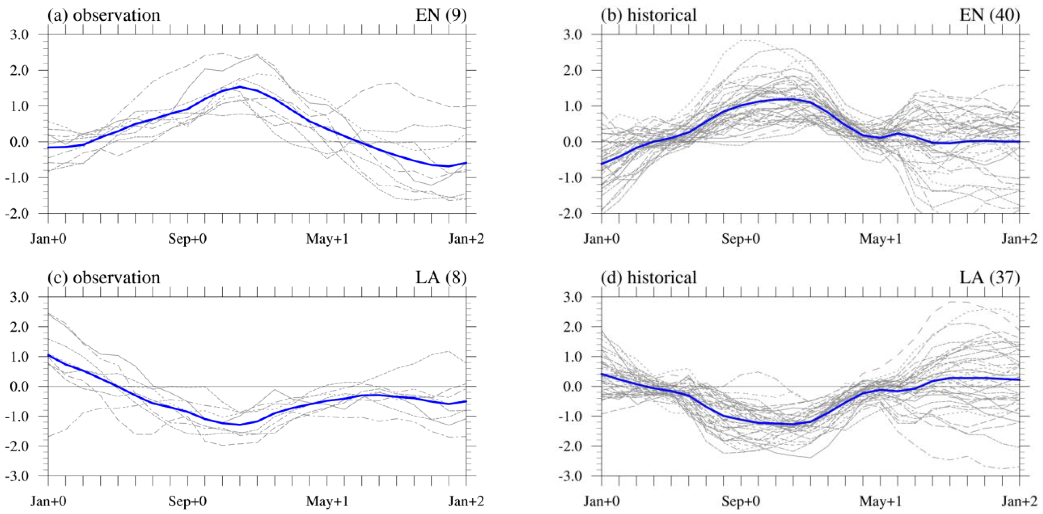
The observed and simulated evolutions of the composite El Niño and La Niña events are shown in Figure 3a,c. The El Niño developing (decaying) year is marked with “+0” (“+1”), respectively. The observed composite Niño3.4 index is positive from April to November of year +0, then decays rapidly after reaching the peak around December and January, and turns negative near July of year +1. Afterwards, a cooling condition begins (Figure 3a). The simple ensemble mean of the historical simulated El Niño usually reaches a peak in December, which is consistent with the observations, but the warming (damping) rate in the developing (decaying) phase seems faster than that in the observations (Figure 3b). Moreover, the observed evolution of La Niña is almost symmetrical to El Niño. It translates to the negative phase in May of year +1 and reaches a peak in the winter, though the composite decaying phase is slower compared to El Niño (Figure 3c). The simulated developing rate of La Niña is close to that in the observations, but it dampens much faster compared with the observations, which means that the observed long persistence of La Niña is not reproduced. Although there is some discrepancy in the magnitude and damping rate, the model generally captures the above observed features.
Maintenance of the equatorial westerly anomaly is necessary for the occurrence of an El Niño event. The equatorial westerly anomalies overlie the climatological easterly and excite a warm oceanic Kelvin wave, which pushes the accumulated warm water in the Western Pacific to propagate eastward.
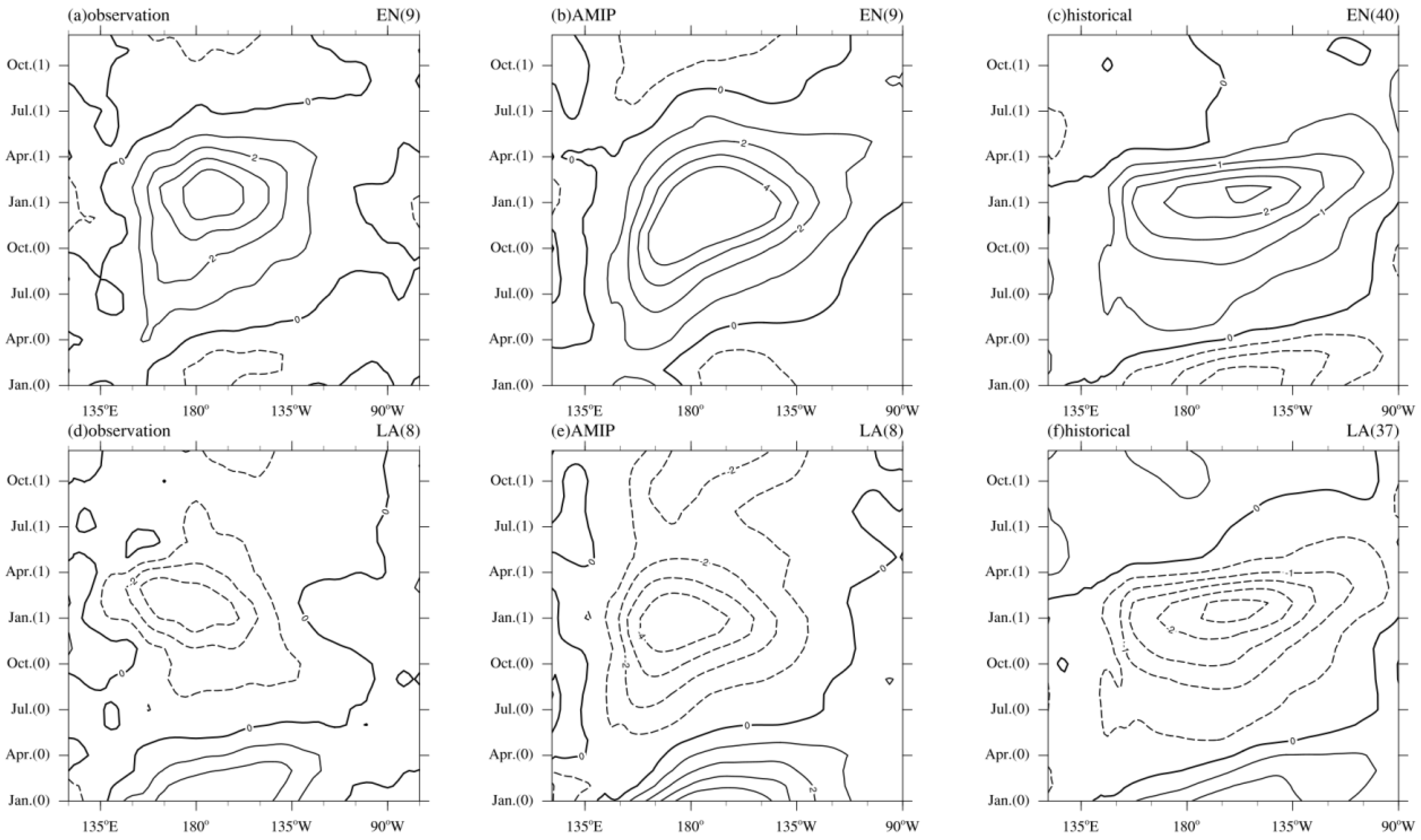
As shown in Figure 4a, in April of the EN developing phase, the westerly anomalies appear in the equatorial Western Pacific, and its location adjusts eastward gradually with the maturity of the warm SST signal. Compared with the observations, the AMIP simulations perform an enhancing process from April to July of year +0, but the maximum westerly anomalies are larger and earlier than those observed (Figure 4b). From the coupled simulations, the occurrence of westerly anomalies is consistent with the observations. However, the westerly anomalies intensify slowly and decay rapidly, associated with eastward propagation (Figure 4c). In the LN event, the easterly anomalies start in the equatorial Western Pacific in the summer of year +0 and ends around July of year +1 (Figure 4d). The easterly anomalies simulated by the AMIP start earlier and end later, so the persistence of the easterly anomaly is longer than that observed (Figure 4e). Unfortunately, in the coupled simulations, the easterly anomalies are still located eastward and still show faster damping (Figure 4f), similar to Figure 4c.

3.2. The East Asian Summer Monsoon Simulated by CAS-ESM2

After examining the composites for the ENSO years, the climatological features of the EASM simulated by CAS-ESM2 and its atmospheric component were evaluated for the common period 1979–2014. Figure 5 shows the summer mean precipitation and 850 hPa circulation in the observations and simulations, along with the model bias (simulation minus observation).
In the observations, an anticyclone circulation resides in the Western North Pacific (WNP), which is known as the WPSH. Precipitation is along the flank of the WPSH (Figure 5a). In the AMIP simulations, the convection in the Philippine Sea has been overestimated compared with the observations (Figure 5b,d). Associated with the convection bias, a cyclonic circulation bias exists south of Japan. The WPSH is located more eastward compared with the observations (Figure 5b). The coupled model can largely reduce this bias, including precipitation and low-level circulation (Figure 5c,e,f). As explored in previous studies, air–sea interaction processes are important in the East Asia and WNP region, and they contribute to this improvement in the performance of the AMIP and coupled models [47].
To examine the interannual variability in the simulation, Figure 6 shows the interannual SDs of the summer mean precipitation in the East Asia and WNP region. In the observations, the SDs are larger along the edge of the WPSH than under the WPSH, which is associated with the interannual eastward/westward movement of WPSH (Figure 6a). In the AMIP simulations, the maximum SD centers are located in the South China Sea (SCS) and the Philippine Sea, associated with the overestimated convection there (Figure 6b). Moreover, the mid-latitude SDs are underestimated (Figure 6d). With respect to the coupled simulations, although the overall magnitude of the SDs has been underestimated (especially for the Philippine Sea), the pattern of the observed SD can be improved compared with the AMIP simulations. That is, the SDs are larger along the edge of the WPSH than under it (Figure 6c). In addition, the underestimated mid-latitude variability in the AMIP simulations can be improved in the coupled simulation (Figure 6e,f). The interannual variability in East China and Northeast China can be realistically reproduced in the coupled model.

3.3. The East Asian Summer Monsoon Related to ENSO Simulated by CAS-ESM2

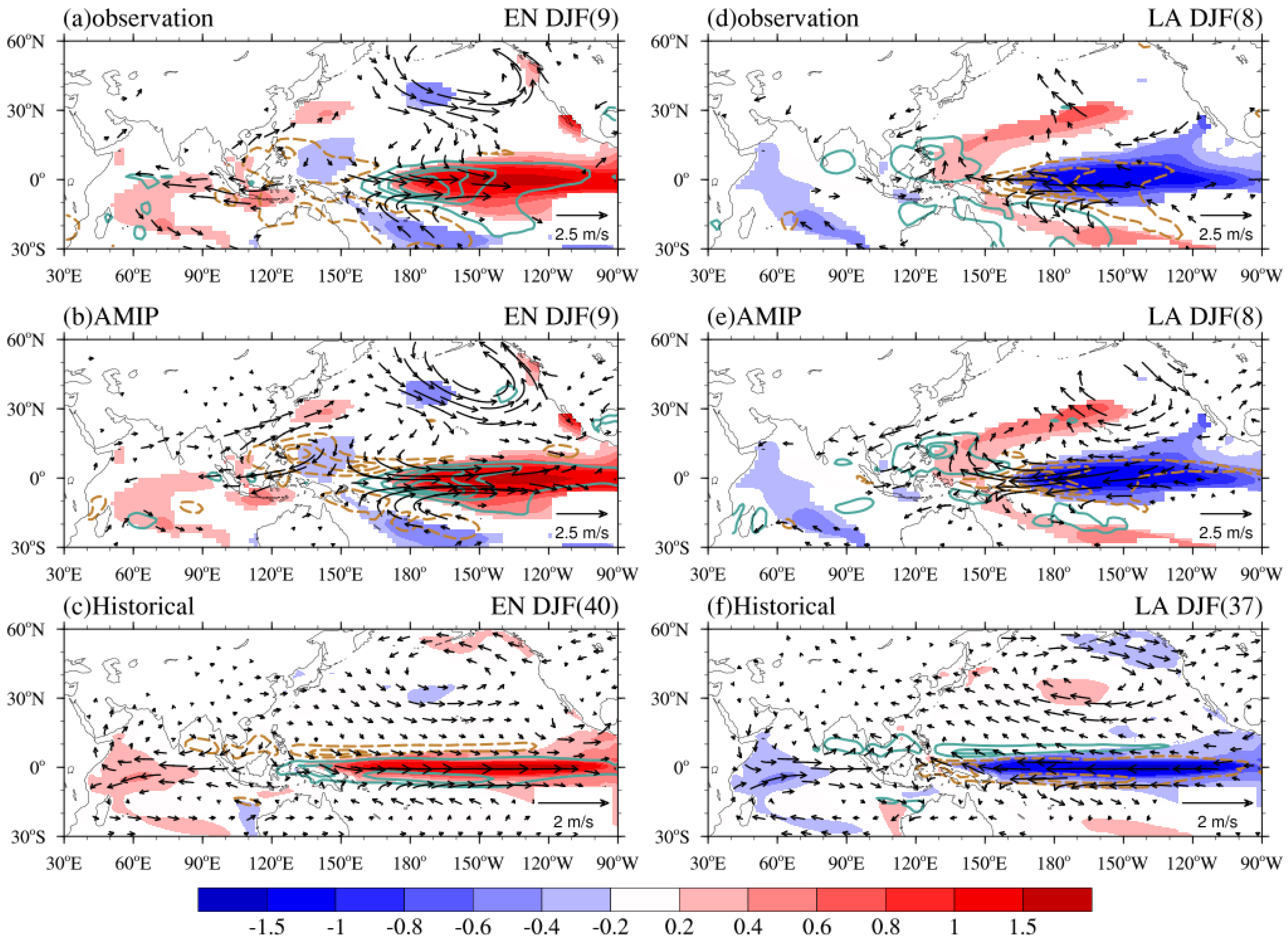
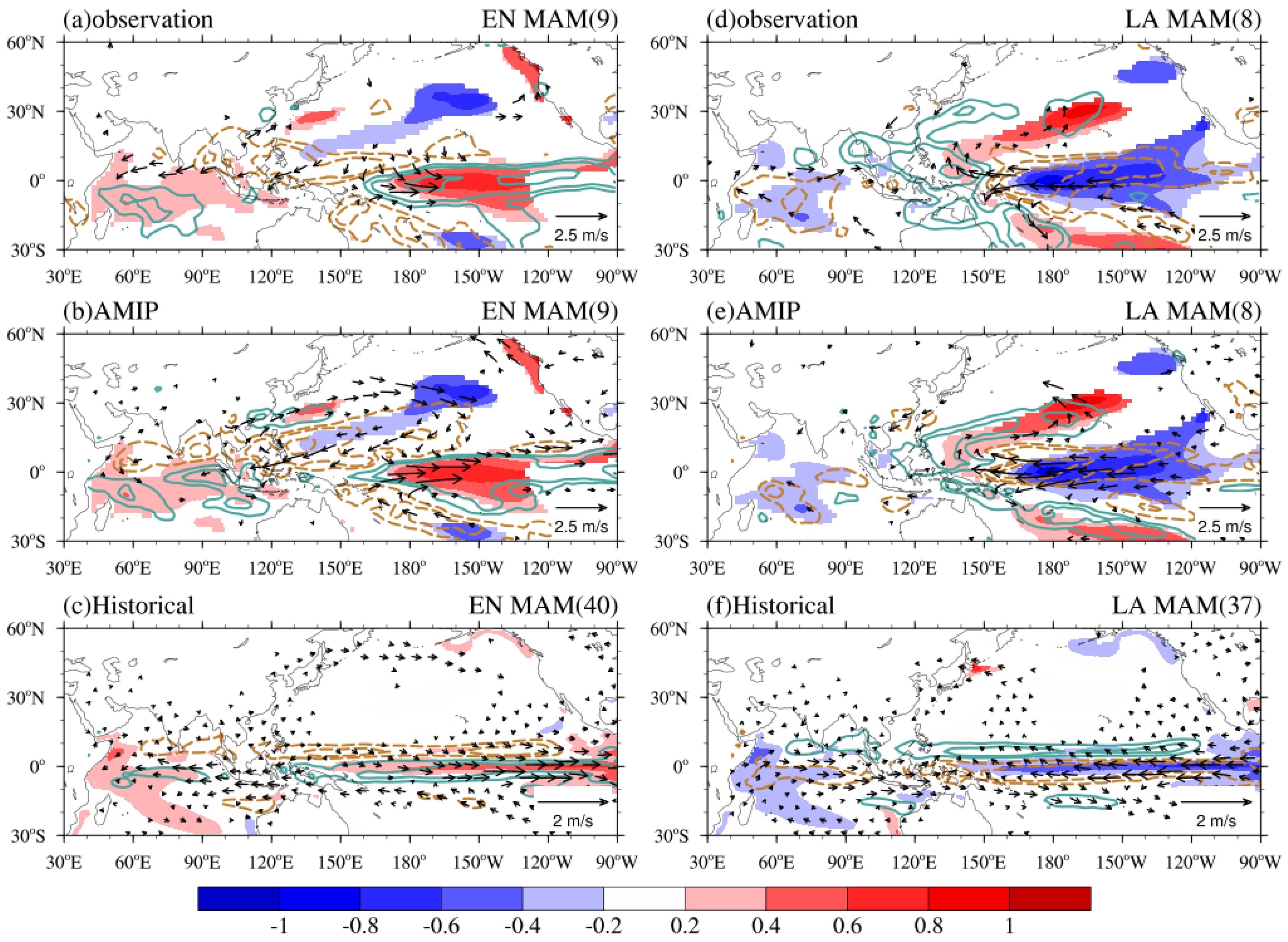
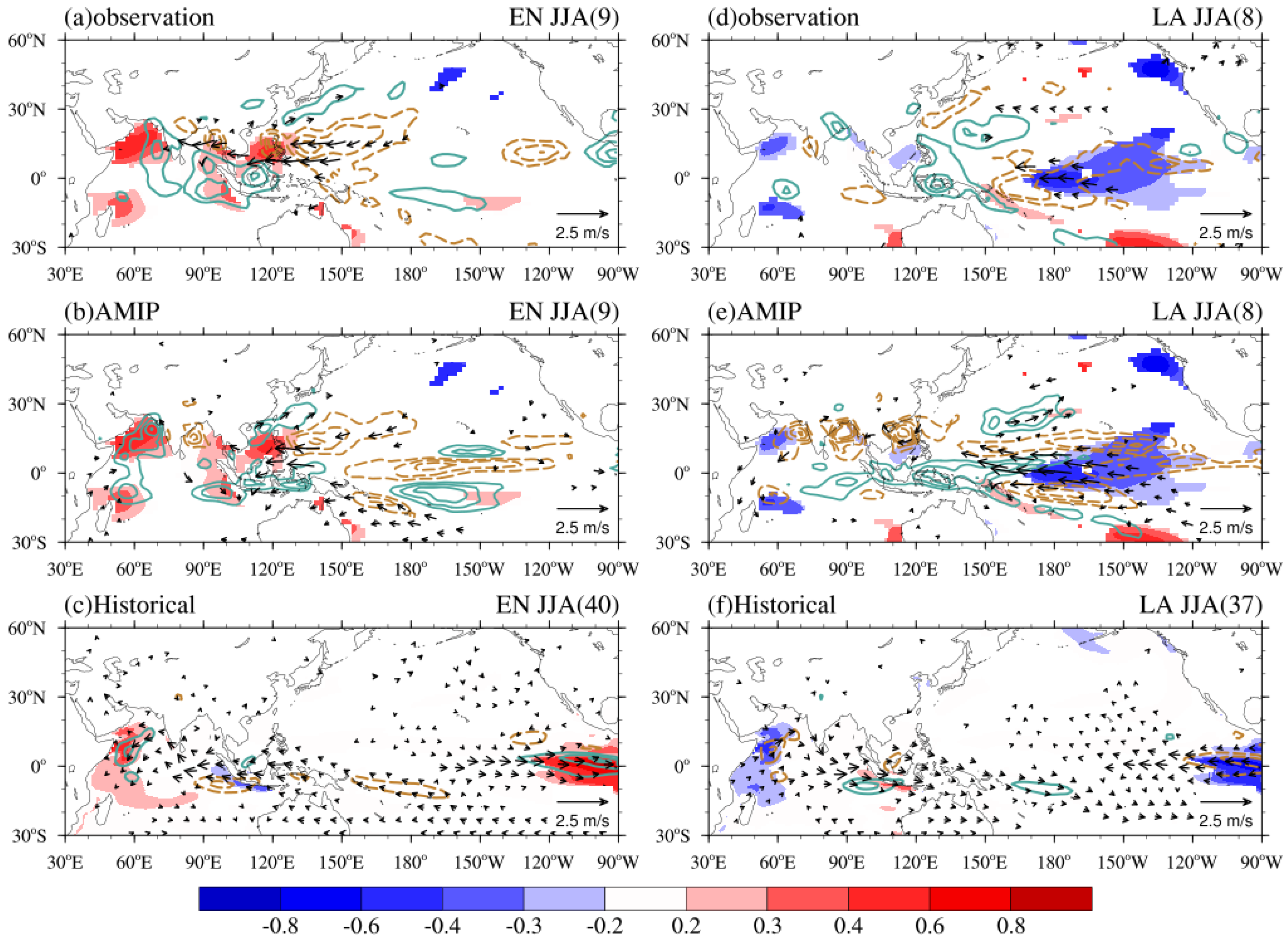
In this section, the evolution of SST, precipitation, and low atmospheric wind anomalies from the mature winter to the decaying summer in the EN and LN years are presented, including the observations and the AMIP and coupled simulations (Figure 7, Figure 8 and Figure 9).
For the observational composite mature winter of EN (Figure 7a), the most pronounced SST signal is the warm SST anomalies in the tropical Central to Eastern Pacific, and the cold SST anomalies occur in the tropical Western Pacific and the Maritime Continent. Other obvious SST anomalies exist in the Indian Ocean, exhibiting basin-wide warming. Corresponding to the Central to Eastern Pacific warming, an abnormal Walker circulation appears in the equatorial Pacific, with anomalous ascending (descending) motion in the equatorial Central Pacific (Maritime Continent). Thus, the more (less) precipitation in the Central (Western) Pacific is a direct response to the anomalous heating associated with El Niño. Correspondingly, there are low-level westerly wind anomalies over the equatorial central and easterly wind anomalies over the Indian Ocean. The WNP is dominated by an anomalous anticyclone, which is coupled with the cold SST anomalies through the wind–evaporation–SST feedback, resulting in less precipitation. It should be highlighted that the maintenance of the Western North Pacific anomalous anticyclone (WNPAC) is a critical connection between El Niño and the EASM.
Based on the AMIP simulations, the WNPAC can be reproduced to an extent, but the westerly anomalies and the associated precipitation anomalies over the equatorial Central Eastern Pacific is stronger than those observed and can reach the East Pacific (Figure 7b). However, in the historical simulations, the performance of the coupled model still has considerable bias. Firstly, the WNPAC is significantly weakened. Secondly, the precipitation anomalies are largely underestimated in magnitude and more concentrated in the equator (Figure 7c). The positional bias may be caused by the further westward extension of the positive SST anomalies.
During the observational mature winter of LN years (Figure 7a), on the contrary, there are cold SST anomalies in the tropical Central to Eastern Pacific, and the warm SST anomalies distribute on the northwest and southwest sides of the cold SST anomalies. Moreover, there is a robust cooling SST signal appearing in the Indian Ocean, showing a negative phase of basin-wide cooling (IOBW). Over the WNP, the anomalous cyclone (WNPC) is shifted westward and weaker compared with the WNPAC during the EN years, and the equatorial region is dominated by easterly anomalies. Coupled with the SST anomalies pattern in the tropical Pacific, which is warm in the west and cold in the central and eastern part, less precipitation appears over the equatorial Central to Eastern Pacific, while the eastern part of the Maritime Continent experiences much precipitation.
The distinguished features of precipitation anomalies and low-level circulation anomalies over the WNP simulated by the AMIP are as significant as that in the observations (Figure 7e), except for an enhanced anomalous anticyclone over the North Pacific. The main discrepancy of the historical simulations is that the cold SST anomalies extend excessively westward, and the zonal structures are much narrower compared with the observations. Accordingly, the anomalous cyclone is more westward than the observations, located over the west of the Indian Ocean, which leads to false location of precipitation (Figure 7f).
In the decaying spring of EN years, the SST signal begins to damp. The warm SST anomalies are significant east of the dateline in the tropical Pacific; meanwhile, the coupled easterly wind anomalies are confined to west of 150° W over the tropical Pacific. Moreover, the amplitude of SST anomalies in the tropical Pacific is weaker than that in the mature winter, while in the Indian Ocean it tends to enhance. The WNPAC is weaker, and the southwesterly anomalies to the northwestern flank of this anomalous anticyclone transport some moisture and enhance the precipitation over Southeastern China (Figure 8a).
For AMIP simulations, the WNPAC is not reproduced well, extends further eastward, and is stronger than that in the observations. Affected by this biased anomalous anticyclone, the area with fewer precipitation anomalies over the Western Pacific is markedly expanded, while the positive precipitation anomalies over Southeastern China can be realistically reproduced (Figure 8b). In the historical simulations, the SST anomalies in the Central and Eastern Pacific are characterized by bias features from winter to spring, with the SST anomalies extending eastward and limited to the equator, so the precipitation is simulated unrealistically (Figure 8c).
With the decaying of cold SST anomalies in the spring of LN, the maximum cold SST anomalies is clearly weakened, with the southwest to northeast extending of warm SST anomalies near the Philippine Sea. Corresponding to this cooling SST, the related lesser precipitation zones over the equatorial Central Eastern Pacific are located to the west of the high-precipitation anomalies associated with EN, reflecting asymmetrical properties. Meanwhile, the WNPC is weaker than that in the mature winter, and the eastern part of the Maritime Continent suffers severe convection and more precipitation induced by warming SST. At the same time, the convection over the Southwest Indian Ocean is suppressed (Figure 8d).
Different from the spring WNPAC in EN simulated by the AMIP (Figure 8e), the crucial WNPC in LN does not show an extending trend to the North Pacific but is closely similar to the observations, and the precipitation anomalies are better reproduced in turn. In the historical simulations, the above anomalous cyclone over the WNP is extend northward, and the magnitude is weaker. The precipitation anomaly distribution shows a symmetry from north to south (Figure 8f).
In the observations, the SST anomalies rapidly decay from the mature winter to the summer, and the warm SST signal in the tropical Central to Eastern Pacific is close to normal, with warm SST anomalies occupying the WNP and SCS instead of the cooling SST in the winter and spring. Meanwhile, the WNPAC persists from the mature winter to the following spring and summer. The equatorial easterly anomalies in the southern flank of this WNPAC reduce the mean monsoon westerly and decrease the surface wind speed, therefore weakening the surface latent heat flux together with the increased the shortwave radiation, leading to warming SST in the WNP. In addition, the WNPAC corresponds to the westward extension of the WPSH, which has a significant impact on precipitation in East Asia. The area with less precipitation extends from the SCS to the Central North Pacific, while many precipitation anomalies are located in the Yangtze River Basin and the Indian Ocean (Figure 9a).
In the AMIP simulations, the WNPAC is located eastward relative to the observations, the magnitude of the former being weaker. Accordingly, the related precipitation anomalies move eastward and are located over the south of the Philippine Sea (Figure 9b). However, the coupled simulations hardly reproduce the above features. On the one hand, there are still strong warm SST anomalies in the equatorial Eastern Pacific with obvious westerly anomalies. On the other hand, the pronounced anomalous anticyclone is located westward (Figure 9c), which leads to a discrepancy in the precipitation pattern. What is more, there are weak negative SST anomalies located in the Eastern Indian Ocean, which is contrary to the observed warming SST, which may be one of the reasons for the further amplification of the simulated bias.
Slightly different from the El Niño in the decaying summer, there are cold SST anomalies in the Central to Eastern Pacific. The maximum cold SST anomalies are near the dateline with easterly anomalies, while the warm SST anomalies near the Philippine Sea vanish in the summer. In the meantime, the WNPC is more northerly, and a weak anomalous anticyclone is established over Northeast Japan, which corresponds to a positive Pacific–Japan pattern [48,49]. Many precipitation anomalies persist over the eastern part of the Maritime Continent, while fewer precipitation anomalies appear over Japan, corresponding to the aforementioned Pacific–Japan Pattern with convection over the subtropical Western Pacific and suppressed convection over Japan (Figure 9d).
On the whole, the AMIP simulations can describe the features of low-level circulation anomalies and precipitation anomalies, but there are still some biases, which is reflected in the stronger easterly anomalies over the Central Pacific and the fewer precipitation anomalies over the SCS (Figure 9e). In the coupled historical simulations, the cooling SST signal is limited to the tropical Eastern Pacific, which is inconsistent with the observations. Therefore, the coupled easterly anomalies are weaker and more easterly than the observations, resulting in a deviation in the falling area of precipitation (Figure 9f).
In the EN decaying summers, the WPSH extends westward consistently throughout the whole summer compared with the climatology (Figure 10a–c). The westward WPSH is associated with suppressed local convection, as represented by the positive precipitation anomalies over the WNP. Associated with the suppressed convection, there is an anticyclonic circulation in the lower level (850 hPa). It is noted that the suppressed convection center tends to shift northward and eastward from June to August, along with the seasonal march of the monsoon circulation.
In the AMIP simulations, the westward extension of WPSH can be reproduced to some extent, especially in June and July (Figure 10d,e). However, the suppressed convection center is not well reproduced compared with the observations. However, with the second subseasonal northward jumping of the WPSH, the simulated circulation markedly decreases. The largest bias is in August (Figure 10f), in which the westward extension of WPSH cannot be realistically reproduced, induced by the underestimated convection weakening in WNP. One reason for the poor performance in the AMIP simulations in the WNP is the lack of air–sea coupling [47]. We find in the historical simulations, however, that the performance of the model of EN decaying summers cannot be improved (Figure 10g–i). However, the coupled model could still capture the process characteristics of the WPSH from June to July, particularly the lower precipitation on the south flank of the WPSH. Meanwhile, the area with more precipitation in Southern China presents a northward movement, similar to the observations. Undeniably, there are some biases in this coupled run. The reasons for the discrepancy may result from the model bias in ENSO simulation, e.g., the overly westward-displaced cold tongue in equatorial regions. The observed EN events tended to shift into LN events in the following year, while the equatorial Pacific in the EN decaying summers remains in normal conditions in the simulations (Figure 3a,b).
In the LN years, the cold conditions in the equatorial Central and Eastern Pacific persist from the mature winter to the summer. In the WNP, convection activity tends to enhance associated with a local warmer SST, resulting in the eastward retreat of the WPSH, especially in July. An anomalous cyclone resides in the lower level, with increased local precipitation.
In the AMIP simulations, the enhanced convection shifts eastward with a weaker magnitude than the observations. Although the enhanced convection can be reproduced to some extent, its subseasonal variation has considerable bias. The simulated enhancement of the convection seems to occur in June, rather than observed July. The largest bias in the AMIP simulations is the overestimated weakening of the convection in the SCS. Compared with the poor performance of the EN decaying summers in the historical simulations, the coupled simulations of the LN years outperform those of the AMIP. First, the overestimated convection weakening in the SCS region is improved in the coupled run. Second, the eastward retreat of the WPSH in the LN summers along with the enhanced convection activity south of Japan can be reproduced to some extent, especially in July. The location bias in the AMIP simulations (eastward-shifted convection enhancement) is also improved in the coupled simulations. The improved performance in the LN years simulated by the historical rather than the AMIP simulations indicates that the air–sea coupling processes may be more important. Further efforts should be conducted to explore whether this conclusion holds in the other CMIP6 models.

4. Conclusions and Discussion

In this study, simulations of the EASM in the EN and LN years by CAS-ESM2 and its atmospheric component have been systematically analyzed. The major conclusions are summarized as follows:
(1) The coupled model generally simulates the annual cycle and interannual variability in the SST in the tropical Pacific, i.e., the 1.5–3-year period. Moreover, the simulated ENSO evolution is analogous to that in the observations, especially for the phase locking. Typically, ENSO events begin in the spring, peak in the mature winter, decay quickly in the following spring, and vanish in the summer. However, the rate of development and attenuation in the simulated ENSO is faster than what is observed; that is to say, the persistence of the ENSO developing and decaying phase is shorter.
Moreover, with both AMIP and historical simulations, the model realistically reproduces a prerequisite for the occurrence of ENSO events and the westerly/easterly anomalies in the equatorial Western Pacific, though there is a tendency in faster damping along with the eastward propagation, which may be related to the depth of the thermocline in the model [50].
(2) Although the climatological precipitation centers and circulation can be reproduced in the AMIP simulations, including the low-level anticyclone circulation corresponding to the WPSH and the precipitation at the edge of the WPSH, the coupled model run can further improve performance; i.e., the overestimated convection in the Philippine Sea and the related cyclonic circulation bias are largely reduced, as revealed in previous studies [24]. With respect to the interannual variability in the EASM, the coupled run presents an observed SDs pattern, in which the SDs along the edge of the WPSH are larger than the SDs below it. Meanwhile, the coupled run can also reduce the mid-latitude bias in the AMIP simulations.
(3) The performance of CAS-ESM2 in simulating low atmospheric circulation and precipitation associated with EN and LN years have been further evaluated from the mature winter to the decaying summer, including the EASM and its subseasonal variation.
The AMIP simulations can capture the circulation characteristics, especially the performance in WNPAC/WNPC, though the westerly/easterly anomalies and the associated precipitation anomalies over the equatorial Central and Eastern Pacific are somewhat overestimated, i.e., with stronger wind anomalies and a more eastward extension. Compared with the AMIP simulations, the performance of the coupled run shows limited improvement.
For the subseasonal simulations, the AMIP run can reproduce the westward extension of the WPSH in the EN summers, though the eastward retreat of the WPSH is weak in the LN summers. In addition, the performance in the simulation of the early summer (June and July) is better than the late summer (August), i.e., corresponding to the westward extension of the WPSH, the distribution pattern of precipitation anomalies is in agreement with the observations.
From the above analysis, we can conclude that, although there is bias in the circulation and precipitation anomalies, the AMIP simulations can realistically reproduce the key characteristics associated with ENSO, especially the performance in WNPAC/WNPC. Thus, new-generation IAP AGCM, like its previous versions, has the potential to be applied in monsoon climate prediction services [51].
As noted in previous studies, air–sea coupling processes are essential to multiscale monsoon variability [23,41,47]. Although air–sea coupling is considered in a coupled model [52,53], it is not necessarily the case that the coupled model outperforms the atmospheric models [54]. The bias in the SST simulation in the coupled models may offset the advantage of considering coupling processes. Considering CAS-ESM2, for example, we found that the bias in ENSO-related SST anomalies limits the ability of the model to realistically reproduce the anomalous EASM associated with ENSO. For instance, the ENSO-related equatorial SST anomaly shifts westward in the coupled model, leading to the westward-shifted easterly anomalies in the equatorial Western Pacific in the EN decaying summers (Figure 9). These anomalies extend from the Western Pacific to the Eastern Indian Ocean. The “wrong” anomalies in the Eastern Indian Ocean result in an upwelling of cold water from the subsurface, forming the local negative SST anomaly. In the observations, the Indian Ocean basin warming in the boreal summer is a key bridge that connects the preceding ENSO and the EASM [55,56]. However, in the coupled model, the “wrong” Eastern Indian Ocean cooling may be a primary cause for the degraded EASM simulation in the coupled model. Thus, improving the coupled model performance (e.g., ENSO) is an imminent task.

Author Contributions

Conceptualization, X.D.; methodology, X.D.; software, W.Z. and X.D.; writing—original draft preparation, W.Z.; writing—review and editing, X.D., J.J., F.X., H.Z., R.L. and W.Z. All authors have read and agreed to the published version of the manuscript.

Funding

This research was jointly supported by the Ning Xia Science Foundation of China (2022AAC03674), the Key Research Program of Frontier Sciences, the Chinese Academy of Sciences (ZDBS-LY-DQC010), and the Youth Innovation Promotion Association of CAS (2022074). The numerical experiment is conducted at “Earth System Science Numerical Simulator Facility” (EarthLab) which is supported by the National Key Scientific and Technological project.

Institutional Review Board Statement

Not applicable.

Informed Consent Statement

Not applicable.

Data Availability Statement

Not applicable.

Conflicts of Interest

The authors declare that there is no conflict of interest.

References

  1. Zhu, K. The enigma of southeast monsoon in China. Acta Geogr. Sin. 1934, 1, 1–27. (In Chinese) [Google Scholar]
  2. Tu, C.; Huang, S. The monsoon advance and retreat in China. Acta Meteorol. Sin. 1944, 18, 81–92. (In Chinese) [Google Scholar]
  3. Ding, Y.H. Summer monsoon rainfall in China. J. Meteorol. Soc. Japan. Ser II 1992, 70, 373–396. [Google Scholar] [CrossRef] [Green Version]
  4. Tao, S.Y.; Chen, L.X. A review of recent research on the East Asian summer monsoon in China. In Monsoon Meteorology; Chang, C.-P., Krishnamurti, T.N., Eds.; Oxford University Press: Oxford, UK, 1987; pp. 60–92. [Google Scholar]
  5. Huang, R.; Zhou, L.; Chen, W. The progresses of recent studies on the variabilities of the East Monsoon and their causes. Adv. Atmos. Sci. 2003, 20, 55–69. [Google Scholar] [CrossRef]
  6. Huang, R.H.; Sun, F.Y. Impact of the tropical western Pacific on the East Asian summer monsoon. J. Meteorol. Soc. Jpn. Ser. II 1992, 70, 243–256. [Google Scholar] [CrossRef] [Green Version]
  7. Dong, X.; Lin, R.; Fan, F. Comparison of the two modes of the western Pacific subtropical high between early and late summer. Atmos. Sci. Lett. 2017, 18, 153–160. [Google Scholar] [CrossRef] [Green Version]
  8. Dong, X.; He, C. Zonal displacement of the western north Pacific subtropical high from early to late summer. Int. J. Climatol. 2020, 40, 5029–5041. [Google Scholar] [CrossRef]
  9. Wu, B.; Zhou, T.; Li, T. Seasonally Evolving Dominant Interannual Variability Modes of East Asian Climate. J. Clim. 2009, 22, 2992–3005. [Google Scholar] [CrossRef]
  10. Huang, R.-H.; Wu, Y.-F. The influence of ENSO on the summer climate change in China and its mechanism. Adv. Atmos. Sci. 1989, 6, 21–33. [Google Scholar]
  11. Ashok, K.; Yamagata, T. Climate change: The El Niño with a difference. Nature 2009, 461, 481–484. [Google Scholar] [CrossRef]
  12. Webster, P.J.; Yang, S. Monsoon and ENSO: Selectively interactive systems. Q. J. R. Meteorol. Soc. 2010, 118, 877–926. [Google Scholar] [CrossRef]
  13. Fu, C.; Teng, X. Climate anomalies in China associated with El Niño/Southern Oscillation. Chin. J. Atmos. Sci. 1988, 12, 133–141. (In Chinese) [Google Scholar]
  14. Zhang, R.H.; Sumi, A.; Kimoto, M. Impact of El Niño on the East Asian monsoon: A diagnostic study of the ‘86/87’ and ‘91/92’ events. J. Meteorol. Soc. Jpn. Ser. II 1996, 74, 49–62. [Google Scholar] [CrossRef] [Green Version]
  15. Xue, F.; Liu, C.-Z. Influence of moderate ENSO on summer precipitation in eastern China and its comparison with strong ENSO. Chin. Sci. Bull. 2007, 52, 2798–2805. (In Chinese) [Google Scholar]
  16. Kawatani, Y.; Ninomiya, K.; Tokioka, T. The north Pacic subtropical high characterized separately for June, July, and August: Zonal displacement associated with submonthly variability. J. Meteorol. Soc. Jpn. Ser. II 2008, 86, 505–530. [Google Scholar] [CrossRef] [Green Version]
  17. Su, T.-H.; Xue, F. Two northward jumps of the summertime western Pacific subtropical high and their associations with the tropical SST anomalies. Atmos. Ocean. Sci. Lett. 2011, 4, 98–102. [Google Scholar]
  18. Wu, B.; Zhou, T.J. Relationships between the East Asian-western north pacific monsoon and ENSO simulated by FGOALS-s2. Adv. Atmos. Sci. 2013, 30, 713–725. [Google Scholar] [CrossRef]
  19. Wu, B.; Zhou, T.J. Relationships between ENSO and the East Asian-western North Pacific monsoon: Observations versus 18 CMIP5 models. J. Clim. 2016, 46, 729–743. [Google Scholar] [CrossRef]
  20. Zhou, T.; Wu, B.; Guo, Z.; Chao, H.; Zou, L.; Chen, X.; Zhang, L.; Man, W.; Li, P.-X.; Li, D.-H. A Review of East Asian Summer Monsoon Simulation and Projection: Achievements and Problems, Opportunities and Challenges. Chin. J. Atmos. Sci. 2018, 42, 902–934. (In Chinese) [Google Scholar]
  21. Zhang, R.-H.; Yu, Y.-Q.; Song, Z.-Y.; Ren, H.-L.; Tang, Y.-M.; Qiao, F.-L.; Wu, T.-W.; Gao, C.; Hu, J.-Y.; Tian, F.; et al. A review of progress in coupled ocean-atmosphere model developments for ENSO studies in China. J. Oceanol. Limnol. 2020, 38, 930–961. [Google Scholar] [CrossRef]
  22. Dong, X.; Fan, F.; Lin, R.; Jin, J.; Lian, R. Simulation of the western north Pacific subtropical high in El Niño decaying summers by CMIP5 AGCMs. Atmos. Ocean. Sci. Lett. 2017, 10, 146–155. [Google Scholar] [CrossRef] [Green Version]
  23. Lin, R.; Dong, X.; Fan, F. Can coupled models perform better in the simulation of sub-seasonal evolution of the western north Pacific subtropical high than atmospheric models in boreal summer? Atmos. Sci. Lett. 2018, 2018, e862. [Google Scholar] [CrossRef] [Green Version]
  24. Dong, X.; Lin, R. Climatological increased precipitation from July to August in the western north Pacific region simulated by CMIP6 models. Atmosphere 2021, 12, 664. [Google Scholar] [CrossRef]
  25. Lin, R.; Zhu, J.; Zheng, F. The application of the SVD method to reduce coupled model biases in seasonal predictions of rainfall. J. Geophys. Res. Atmos. 2019, 124, 11837–11849. [Google Scholar] [CrossRef]
  26. Zhou, Z.-Q.; Xie, S.-P.; Zhang, G.-J.; Zhou, W. Evaluating AMIP skill in simulating interannual variability of summer rainfall over the Indo-Western Pacific. J. Clim. 2018, 31, 2253–2265. [Google Scholar] [CrossRef]
  27. Kanamitsu, M.; Ebisuzaki, W.; Woollen, J.; Yang, S.-K.; Hnilo, J.J.; Fiorino, M.; Potter, G.L. NCEP–DOE AMIP-II Reanalysis (R-2). Bull. Am. Meteorol. Soc. 2002, 83, 1631–1644. [Google Scholar] [CrossRef]
  28. Adler, R.F.; Huffman, G.J.; Chang, A.; Ferraro, R.; Xie, P.-P.; Janowiak, J.; Rudolf, B.; Schneider, U.; Curtis, S.; Bolvin, D.; et al. The Version-2 Global Precipitation Climatology Project (GPCP) Monthly Precipitation Analysis (1979–Present). J. Hydrometeorol. 2003, 4, 1147–1167. [Google Scholar] [CrossRef]
  29. Huang, B.; Thorne, P.W.; Banzon, V.F.; Boyer, T.; Chepurin, G.; Lawrimore, J.H.; Menne, M.J.; Smith, T.M.; Vose, R.S.; Zhang, H.-M. Extended Reconstructed Sea Surface Temperature, Version 5 (ERSSTv5): Upgrades, Validations, and Intercomparisons. J. Clim. 2017, 30, 8179–8205. [Google Scholar] [CrossRef]
  30. Smith, T.M.; Reynolds, R.W.; Peterson, T.C.; Lawrimore, J. Improvements to NOAA’s Historical Merged Land–Ocean Surface Temperature Analysis (1880–2006). J. Clim. 2008, 21, 2283–2296. [Google Scholar] [CrossRef]
  31. Zhang, H.; Zhang, M.; Zeng, Q.-C. Sensitivity of Simulated Climate to Two Atmospheric Models: Interpretation of Differences between Dry Models and Moist Models. Mon. Weather Rev. 2013, 141, 1558–1576. [Google Scholar] [CrossRef]
  32. Liu, H.; Zhang, X.; Li, W.; Yu, Y.-Q. An Eddy-Permitting Oceanic General Circulation Model and Its Preliminary Evaluation. Adv. Atmos. Sci. 2004, 21, 675–690. [Google Scholar]
  33. Dong, X.; Jin, J.-B.; Liu, H.-L.; Zhang, H. CAS-ESM2.0 model datasets for the CMIP6 Ocean Model Intercomparison Project Phase 1 (OMIP1). Adv. Atmos. Sci. 2021, 38, 307–316. [Google Scholar] [CrossRef]
  34. Jin, J.; Zhang, H.; Dong, X.; Liu, H.; Zhang, M.; Gao, X.; He, J.-X.; Chai, Z.; Zeng, Q.; Zhou, G. CAS-ESM2.0 Model Datasets for CMIP6 Flux-Anomaly-Forced Model Intercomparison Project (FAFMIP). Adv. Atmos. Sci. 2021, 38, 296–306. [Google Scholar] [CrossRef]
  35. Dai, Y.-J.; Zeng, X.-B.; Dickinson, R.; Baker, I. The common land model (CLM). Bull. Am. Meteorol. Soc. 2003, 84, 1013–1023. [Google Scholar] [CrossRef] [Green Version]
  36. Ji, D.-Y.; Wang, L.; Feng, J.-M.; Wu, Q.-Z. Description and basic evaluation of Beijing Normal University Earth System Model (BNU-ESM) version 1. Geosci. Model Dev. 2014, 7, 2039–2064. [Google Scholar] [CrossRef] [Green Version]
  37. Hunke, C.H.; Lipscomb, W.H. CICE: The Los Alamos Sea Ice Model Documentation and Software User’s Manual Version 4.0 LA-CC-06-012; Los Alamos National Laboratory: Santa Fe, NM, USA, 2008. [Google Scholar]
  38. Dong, X.; Xue, F.; Zhang, H.; Zeng, Q. Evaluation of surface air temperature change over China and the globe during the twentieth century in IAP AGCM4.0. Atmos. Ocean. Sci. Lett. 2012, 5, 435–438. [Google Scholar]
  39. Dong, X.; Su, T.; Wang, J.; Lin, R. Decadal variation of the Aleutian Low-Icelandic Low seesaw simulated by a climate system model (CAS-ESM-C). Atmos. Ocean. Sci. Lett. 2014, 7, 110–114. [Google Scholar]
  40. Dong, X.; Xue, F. Phase transition of the Pacific decadal oscillation and decadal variation of the East Asian summer monsoon in the 20th century. Adv. Atmos. Sci. 2016, 33, 330–338. [Google Scholar] [CrossRef]
  41. Lin, R.; Zhu, J.; Zheng, F. Decadal shifts of East Asian summer monsoon in a climate model free of explicit GHGs and aerosols. Sci. Rep. 2016, 6, 38546. [Google Scholar] [CrossRef] [Green Version]
  42. Dong, X.; Zheng, F.; Lin, R.-P.; Yang, H.-P. A reasonable mean dynamic topography state on improving the ability of assimilating the altimetry observations into a coupled climate system model: An example with CAS-ESM-C. J. Geophys. Res. Oceans 2021, 126, e2020JC016760. [Google Scholar] [CrossRef]
  43. Eyring, V.; Bony, S.; Meehl, G.A.; Senior, C.; Stevens, R.J.; Stouffer, R.J.; Taylor, K.E. Overview of the coupled model intercomparison project phase 6 (CMIP 6) experimental design and organization. Geosci. Model Dev. 2015, 8, 10539–10583. [Google Scholar]
  44. Zhang, H.; Zhang, M.-H.; Jin, J.-B.; Fei, K. Description and climate simulation performance of CAS-ESM Version 2. J. Adv. Model. Earth Syst. 2020, 12, e2020MS002210. [Google Scholar] [CrossRef]
  45. Xue, F.; Dong, X.; Fan, F.-X. Anomalous western Pacific subtropical high in El Niño developing summer and its comparison with the decaying summer. Adv. Atmos. Sci. 2018, 35, 360–367. [Google Scholar] [CrossRef]
  46. Dong, X. Influences of the Pacific Decadal Oscillation on the East Asian Summer Monsoon in non-ENSO years. Atmos. Sci. Lett. 2016, 17, 115–120. [Google Scholar] [CrossRef]
  47. Wang, B.; Ding, Q.; Fu, X.; Kang, I.-S.; Jin, K.; Shukla, J.; Doblas-Reyes, F. Fundamental challenge in simulation and prediction of summer monsoon rainfall. Geophys. Res. Lett. 2005, 32, L15711. [Google Scholar] [CrossRef] [Green Version]
  48. Kosaka, Y.; Nakamura, H. Structure and dynamics of the summertime Pacific-Japan teleconnection pattern. Q. J. R. Meteorol. Soc. 2010, 132, 2009–2030. [Google Scholar] [CrossRef]
  49. Nitta, T. Convective activities in the tropical wetern Pacific and their impact on the northern hemisphere summer circulation. J. Meteorol. Soc. Jpn. Ser. II 1987, 65, 373–390. [Google Scholar] [CrossRef] [Green Version]
  50. Su, T.-H.; Xue, F.; Sun, H.-C.; Zhou, G.-Q. The El Niño-Southern Oscillation cycle simulated by the climate system model of Chinese Academy of Sciences. Acta Oceanol. Sin. 2015, 34, 55–65. [Google Scholar] [CrossRef]
  51. Lin, Z.-H.; Wang, H.-J.; Zhou, G.-Q.; Chen, H.; Lang, X.-M.; Zhao, Y.; Zeng, Q.-C. Recent Advances in Dynamical Extra-Seasonal to Annual Climate Prediction at IAP/CAS. Adv. Atmos. Sci. 2004, 21, 456–466. [Google Scholar]
  52. Zhang, R.-H. A hybrid coupled model for the Pacific ocean-atmosphere system. Part I: Description and basic performance. Adv. Atmos. Sci. 2015, 32, 301–318. [Google Scholar] [CrossRef]
  53. Zhang, R.-H. Structure and effect of ocean biology-induced heating (OBH) in the tropical Pacific, diagnosed from a hybrid coupled model simulation. Clim. Dyn. 2015, 44, 695–715. [Google Scholar] [CrossRef]
  54. Zhang, R.-H.; Gao, C.; Feng, L.C. Recent ENSO evolution and its real-time prediction challenges. Natl. Sci. Rev. 2022, 9, nwac052. [Google Scholar] [CrossRef] [PubMed]
  55. Xie, S.P.; Hu, K.M.; Hafner, J.; Tokinaga, H.; Du, Y.; Huang, G.; Sampe, T. Indian Ocean capacitor effect on Indo-western Pacific climate during the summer following El Niño. J. Clim. 2009, 22, 730–747. [Google Scholar] [CrossRef]
  56. Xie, S.P.; Kosaka, Y.; Du, Y.; Hu, K.; Chowdary, J.S.; Huang, G. Indo-western Pacific ocean capacitor and coherent climate anomalies in post-ENSO summer: A review. Adv. Atmos. Sci. 2016, 33, 411–432. [Google Scholar] [CrossRef] [Green Version]
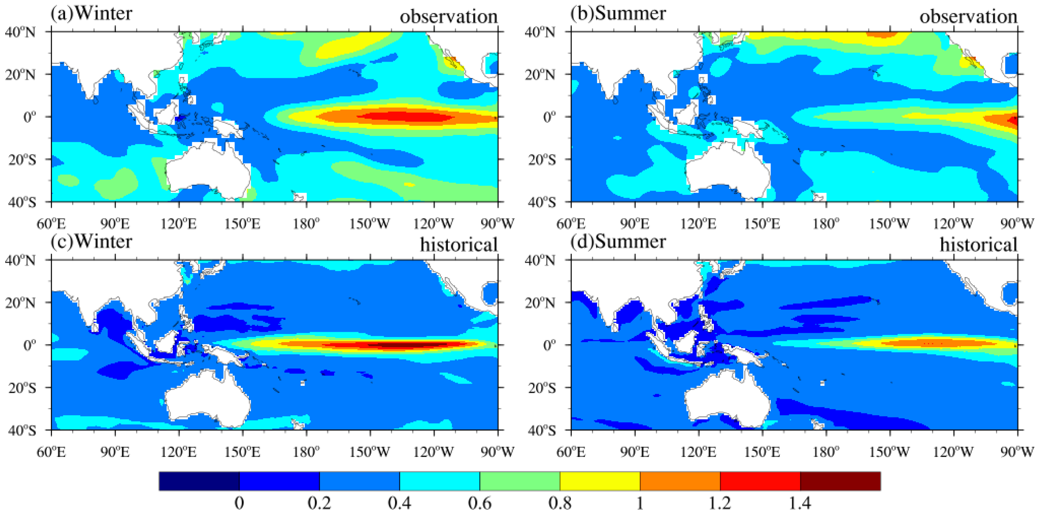
Figure 1. The observed (a,b) and simulated (c,d) standard deviation of the sea surface temperature (units: °C) in the tropical Pacific in the winter (a,c) and the following summer (b,d).
Atmosphere 13 00998 g001
Figure 2. The observed (a) and simulated (b) power spectra of the Niño3.4 index (the black line). The blue dashed line and red line indicate the 0.95 confidence level and the red noise spectrum, respectively.
Atmosphere 13 00998 g002
Figure 3. The observed (a,c) and simulated (b,d) temporal SST anomalies (units: °C) over the Niño3.4 region in the El Niño (a,b) and La Niña (c,d) years. The gray lines represent the individual ENSO events in the observations or simulations, and the thick blue line represents the composite of these ENSO events.
Atmosphere 13 00998 g003
Figure 4. The time-longitude cross-sections of the composite 850 hPa zonal wind (m/s) along the equator in the observations (a,d), AMIP simulations (b,e), and historical simulations (c,f) of the El Niño (ac) and La Niña (de) years. The “0” and “1” in the vertical coordinates represent the developing and decaying years of the El Niño and La Niña, respectively.
Atmosphere 13 00998 g004
Figure 5. Climatological summer mean precipitation (shading, unit: mm/day) and 850 hPa wind field (vectors, unit: m/s) in (a) observations, (b) AMIP simulations, and (c) historical simulations. (d,e) The AMIP and historical bias, respectively. (f) The difference between historical and AMIP simulations.
Atmosphere 13 00998 g005
Figure 6. The interannual standard deviations of summer mean precipitation. (shading) in (a) observations, (b) AMIP simulations, and (c) historical simulations. (d,e) The AMIP and historical bias, respectively. (f) The difference between historical and AMIP simulations.
Atmosphere 13 00998 g006
Figure 7. Composite SST (shaded, unit: °C), wind field at 850 hPa (vectors, unit: m/s), and precipitation anomalies (contour, unit: mm/d) in the El Niño (ac) and La Niña (df) mature winters in the observations (top panels), AMIP simulations (middle panels), and historical simulations (bottom panels). The green solid (yellow dashed) lines denote positive (negative) precipitation values. SST anomalies and wind anomalies exceeding the 10% significance level are shown.
Atmosphere 13 00998 g007
Figure 8. Composite SST (shaded, unit: °C), wind field at 850 hPa (vectors, unit: m/s), and precipitation anomalies (contour, unit: mm/d) in El Niño (ac) and La Niña (df) decaying springs in observations (top panels), AMIP simulations (middle panels), and historical simulations (bottom panels). The green solid (yellow dashed) lines denote positive (negative) precipitation values. SST anomalies and wind anomalies exceeding the 10% significance level are presented.
Atmosphere 13 00998 g008
Figure 9. Composite SST (shaded, unit: °C), wind field at 850 hPa (vectors, unit: m/s), and precipitation anomalies (contour, unit: mm/d) in the El Niño (ac) and La Niña (df) decaying summers in the observations (top panels), AMIP simulations (middle panels), and historical simulations (bottom panels). The green solid (yellow dashed) lines denote positive (negative) precipitation values. SST anomalies and wind anomalies exceeding the 10% significance level are presented.
Atmosphere 13 00998 g009
Figure 10. Composite precipitation anomalies (shading, unit: mm/d), wind field at 850-hPa (vectors, unit: m/s), and WPSH (contour, denoted by 5880 or 5870 gpm geopotential height at 500 hPa, unit: gpm) in El Niño decaying summers in the observations (left panels), AMIP simulations (middle panels), and historical simulations (right panels). (a,d,g) June, (b,e,h) July, and (c,f,i) August. Black (red) line denotes the climatological mean (composite in El Niño decaying years).
Atmosphere 13 00998 g010
Publisher’s Note: MDPI stays neutral with regard to jurisdictional claims in published maps and institutional affiliations.