Combining Spatial and Temporal Data to Create a Fine-Resolution Daily Urban Air Temperature Product from Remote Sensing Land Surface Temperature (LST) Data

Abstract

Remotely sensed land surface temperature (LST) is often used as a proxy for air temperature in urban heat island studies, particularly to illustrate relative temperature differences between locations. Two sensors are used predominantly in the literature, Landsat and Moderate Resolution Imaging Spectroradiometer (MODIS). However, each has shortcomings that currently limit its utility for many urban applications. Landsat has high spatial resolution but low temporal resolution, and may miss hot days, while MODIS has high temporal resolution but low spatial resolution, which is inadequate to represent the fine grain heterogeneity in cities. In this paper, we overcome this inadequacy by combining high spatial frequency Environmental Services (ES), Landsat-driven Normalized Difference Vegetation Index (NDVI), and MODIS low spatial frequency background LST at different spatial frequency bands (spatial spectral composition). The method is able to provide fine scale LST four times daily on any day of the year. Using data from Paris in 2019 we show that (1) daytime cooling by vegetation reaches a maximum of 30 °C, above which there is no further increase in cooling. In addition, (2) the cooling is relatively local and does not extend further than 200 m beyond the boundary of the NBS. This model can be used to quantify the benefits of NBS in providing cooling in cities.

1. Introduction

For detailed studies of the impact of nature-based solutions (NBS) on air temperatures in urban environments, one needs a high spatial resolution distribution of air temperature on multiple days throughout the year. One can use measured temperature profiles [1,2,3,4] but these are limited to single parks or other transects through the city (i.e., sparse geographical information) with sparse temporal measurements. Another option would be to use remotely sensed land surface temperature (LST) since these capture spatial temperature patterns. However, LST requires conversion in some manner to air temperatures to be useful with many other studies of the benefits of NBS and the impacts of high urban air temperatures. For example, the daily mean air temperature has been related to human mortality and health [5] and energy demand for cooling [6]. Adding a spatially continuous proxy for weather station air temperature components on multiple days may improve the results of the analyses and identify hot spots (pun intended). The goal of this methodology is to produce this component (a spatially continuous proxy for weather station air temperatures) using freely available data such as LANDSAT and MODIS remote sensing products and weather station temperature records, for example from NOAA or the national weather service.

However, to reach this desired goal, two hurdles must be overcome: (1) LST with high spatial resolution tends to have a low temporal resolution, and vice versa, and (2) the relationship between LST to air temperature is not straightforward. Therefore, the goal is approached in two phases. Firstly, a new method for producing high spatial frequency LST on a daily basis will be presented (overcoming the first hurdle). Thereafter, these intermediary products, daily high spatial frequency LST, will be used to build a relationship with daily weather station air temperature indicators and this relationship will be applied to the intermediary product to create a modelled or “synthetic” spatially continuous weather station air temperature. For consistency, in the remainder of this paper air temperature has the meaning of weather station based air temperature. This should not be confused with air temperature measured in situ or other measurements of thermal comfort (e.g., Physiological Equivalent Temperature index [7]).

Two sensors, LANDSAT and MODIS, are used predominantly in the literature for LST studies. However, these two have shortcomings. LANDSAT has a high spatial resolution (100 to 120 m, resampled to 30 m × 30 m) but a low temporal resolution (every 16 days), and MODIS has a high temporal resolution (four-times daily) but a low spatial resolution (1000 m × 1000 m). The low temporal resolution of LANDSAT and the presence of clouds mean that there are often very few images of a specific location available per year, and the 16-day interval means that individual hot days, which are often a focus for studying the impacts of extreme events may not always be represented. The temporal interval of the MODIS images is well suited to capturing temperature variation at sub-daily scales, but their spatial coarseness makes them unsuitable in fine-grained highly heterogeneous urban settings.

To overcome these limitations, methods have been developed to produce high spatial resolution LST images at frequent temporal resolution. The most commonly used of these methods are the disaggregation procedure for radiometric surface temperature (DisTrad) [8] and the algorithm for sharpening thermal imagery (TsHARP) [9]. Both these methods use the observed linear relationship between LST and the normalized difference vegetation index (NDVI) to generate the high spatial resolution LST from the existing high resolution (NDVI). These methods assume that the linear relationship does not change over the study region. Subsequently, methods that are more complicated have been developed which improve the accuracy of the downscaling and remove the spatially invariant assumption. These methods include using additional independent variables [10,11] or geographic variability [12]. In all studies, the downscaled product is compared with the high resolution LANDSAT LST. None of these methods attempt to mix LST data from the two sources.

In the present study, we propose a new approach to addressing the first hurdle by postulating that there are three components to the spatial variation of LST in urban environments: (1) a mean level controlled by the time of day and year, and weather; (2) a low spatial frequency component controlled by the broad-scale structure of the city and surface elevation; and (3) a high spatial frequency component that results from the addition of NBS in the city. The downscaling methodology does not need to address the first two spatial components. The mean temperature is available from weather stations throughout a city. MODIS instruments measure the long wavelength LST component four times daily. Hence, the problem can be simplified to mixing a short wavelength “differential” LST calculated using a DisTrad approach to the long wavelength MODIS LST.

For the second hurdle, many studies using MODIS LST have already shown a correlation with air temperature [13,14,15,16,17,18]. Generally, these studies have found that the correlation tends to be good for winter months and nighttime in summer months. The correlation is poorer for daytime in the summer months. There is a tendency for MODIS LST to overestimate the air temperature in non-forested areas. This result should not be surprising since the MODIS LST is a 1000 m × 1000 m sample, and the air temperature is a point measurement on a grassy area at least 4 m away from a building or other structure.

Of more interest to the present paper are studies investigating the relationship between LANDSAT LST and air temperature. These studies are much fewer in number. In a regional study, Goldblatt et al. [19] develop a multiple linear regression model for predicting air temperature which includes LST, NDVI, surface albedo, elevation, and Julian day. For a small geographic area, they found significant linear relationships between in-situ air temperature and LST alone and LST plus other variables at different spatial locations on 2 days. This result was found even though the days of in-situ measurements and the LANDSAT flyovers did not coincide exactly.

Study Objectives

To summarise, the purpose of this study is to develop a robust method to (1) create a fine-spatial resolution product of air temperature (daily mean and maximum) based on publicly available data (LANDSAT and MODIS images and weather station based temperatures) on any day of the year, (2) apply this method to evaluate the benefits of urban vegetation in parks in Paris, to demonstrate the potential of such NBS to provide urban cooling.

The structure of the paper is as follows: first, the methodology is developed in detail. The method creates high spatial resolution LSTs using an extension to the accepted DisTrad approach as interim products. The method then converts these interim products to air temperature (daily mean and maximum) assuming that the relationship between LST and air temperature throughout the year is similar to the relationship on a specific day (similar to the concept of ergodicity in geology). Secondly, results are presented after each processing step. Finally, the main results and their implications are discussed before drawing a conclusion.

2. Materials and Methods

2.1. Study Area

The study area is Île-de-France/Paris region (1.53° E–3.49° E, 47.99° N–49.48° N). Île-de-France is the administrative region around France’s national capital, Paris. The region has a population of roughly 12.2 million inhabitants and over 25,000 inhabitants per 5 km² [20]. The topography of the region is one of the low hills surrounding the Seine River valley. The minimum and maximum elevations are 56 m and 183 m respectively. Paris has average daily temperatures of 4.3 °C in January to 19.8 °C in July. However, the average maximum temperatures in July are 24.2 °C. In 2019, Orly Airport reported a then-record daily maximum temperature of 42.4 °C on July 25 (day 206). Paris typically has gentle breezes of 15–18 km/h for most of the year, with slightly higher wind speeds in winter months. The wind direction in summer is predominantly from the west although in summer 2019 the wind was southerly.

2.2. Datasets

Remote sensing data are from all MODIS Aqua and Terra daytime LST and NDVI with low cloud cover from 2019. The two sensors record different LST since Aqua has flyovers in mid-afternoon and the Terra images are from around 13:00. The spatial resolution of the images is 1000 m × 1000 m. Each image consists of 163 × 172 = 28, 036 pixels.

In addition, we used five LANDSAT 8 images from 2019 (days 57, 89, 153, 185, and 249). All datasets are from LANDSAT 8, with OLI and TIRS bands, with a processing level C1 Level-1. These images have a spatial resolution of 30 m × 30 m and consist of 5017 × 5351 = 26,845,967 pixels. LANDSAT flyovers are around mid-day.

Very little weather data is publicly available for the region. Two stations, Orly Airport (NOAA Station ID FRM00007149, 48.7167 °N, 2.3842 °E, elevation 89 m) and Le Bourget (NOAA Station ID: GHCND:FRM00007150, 48.9675 °N, 2.4275 °E, elevation 67 m), from NOAA Climate Data Online (https://www.ncdc.noaa.gov/cdo-web/, accessed on 14 July 2022), were used.

2.3. Approach

The methodology presented consists of four steps:

• Creating temperature variable DisTrad functions for a specific MODIS sensor (i.e., Aqua or Terra)
• Generating day-specific high resolution simple DisTrad LST
• Calculating day-specific high-resolution synthetic LST using a spatial band-width composition, including the application of a correction (blurring) filter, and
• Converting the day-specific high-resolution synthetic LST to a modeled air temperature by applying linear regression against known weather stations

A quantitative comparison of the processing steps to the LANDSAT LST is not straightforward since the MODIS-based products occur at a different time than the LANDSAT LST. Hence, there is a bias that is inherent in the comparison. For comparison, root mean square error (RMSE) is shown after each processing step with the assumption that the processing step is a model, and the LANDSAT LST is the observed data. In addition, since there may be outliers the mean absolute error (MAE) may also be calculated. In order to accommodate and correct for the bias, two sets of indicators at each step are shown: without correction, and with correction by subtracting the mean for the processed data and adding the mean LANDSAT LST.

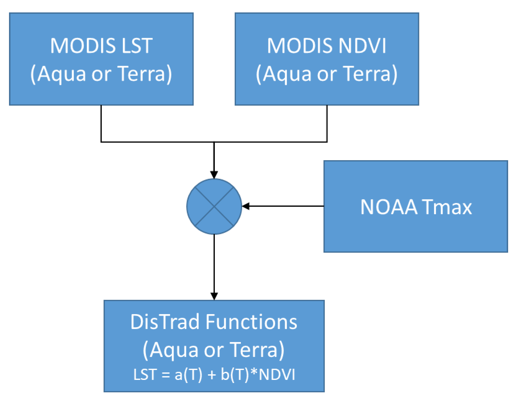
Figure 1 shows the flow for the first step. For all days in the study year, a linear regression is performed between MODIS NDVI (predictor) and LST (response).

LST = a + b NDVI

(1)

All pixels are used in the regression. The regression parameters (intercept and slope) are then combined with the daily maximum temperature (NOAA T_max) to create functions that predict the DisTrad intercept and slope for any daily maximum temperature. The form of these functions will be discussed in the results section. Because LST is strongly affected by clouds and recent precipitation [21], care must be taken to remove poor data from further analysis. Only scenes with more than 50% non-cloud, and with the percentage standard error intercept or slope < 25% were included to form the functions.

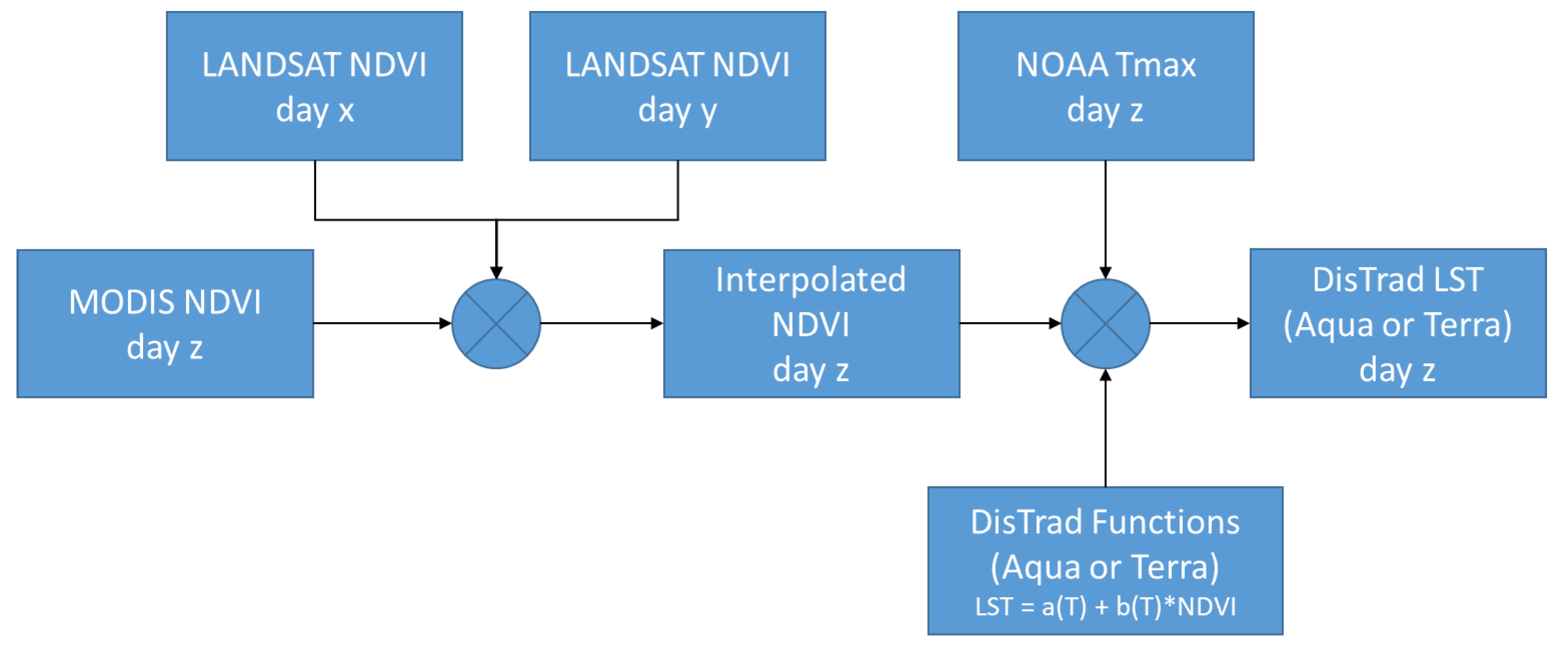
In the second step, LANDSAT NDVI for all available days was calculated using the Mono-Window Algorithm (MWA) described in Wang et al. [22]. To find the high resolution NDVI on a specific day (z), adjacent LANDSAT NDVI were linearly interpolated (days x and y) and adjusted using the average MODIS NDVI on a specific day. This is designated the interpolated NDVI in Figure 2. This raster, in combination with the maximum temperature (T_max) for the day and the temperature dependent DisTrad functions, was used to create a high resolution DisTrad LST for the specified day and time, as illustrated schematically in Figure 3.

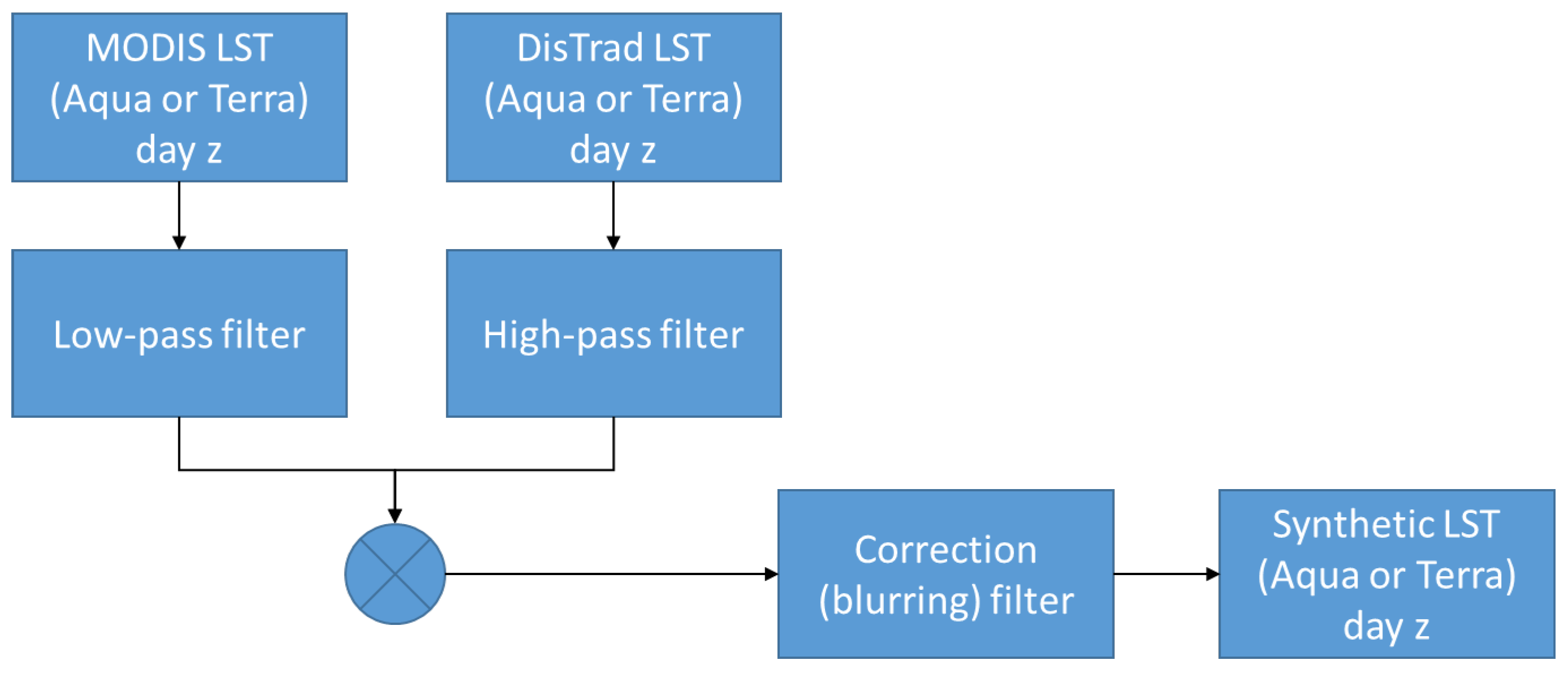
During the analysis, it became apparent that the MODIS and DisTrad LSTs have quite different spatial power spectra. The MODIS LST is rich in low and poor in high spatial frequencies. The DisTrad LST has the reverse relationship. However, a simple summing of the two products may overestimate the entire spectrum. Hence, a low-pass spatial filter using a circular equal weight average filter is applied to the day-specific MODIS LST. The same filter is applied to the day-specific DisTrad LST. However, the filtered product is subtracted from the DisTrad LST and results in a high-pass spatially filtered version of the DisTrad LST.

One can compare this spatial bandwidth composed product with different filter radii with LANDSAT LST to choose an optimal filter radius. For this purpose, the LANDSAT LST was calculated using the Split Window Algorithm (SWA) described in Rozenstein et al. [23].

Even with optimal bandwidth composition, the power spectrum of the composed product does not match the power spectrum of the LANDSAT LST. The composed product is still too rich in high spatial frequencies as compared to the LANDSAT LST. Hence, a correction filter is estimated using naïve deconvolution [24] for each day with a LANDSAT LST. The correction filters are averaged, and the average filter is applied to the day-specific composed product to create the synthetic LST. The step is related to algorithms for deblurring photos, but the blurring filter is estimated and applied purposely to blur the composed LST. More complicated algorithms could be used that rely on a priori knowledge of the approximate signal-to-noise ratio (e.g., Wiener deconvolution [24]. However, in our experience, the naïve deconvolution results were very stable. The processing flow up to here enables the user to generate a high-resolution synthetic LST for potentially any day of the year.

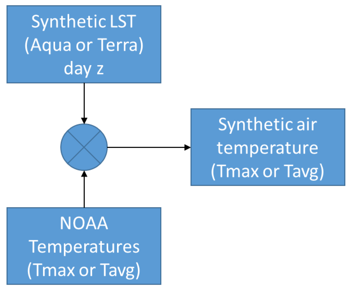
With a continuous range of days with synthetic LST products throughout the year, it is possible to define a relationship between the LST and air temperature at weather stations (Figure 4). This is especially valuable since weather/synoptic stations serve as reference points to verify the results. Since, in Europe, MODIS Aqua passes overhead in mid-afternoon, the Aqua-based synthetic LST can be related to T_max. The Terra-based synthetic LST can be used to predict T_ave. The parameters defining the relationships can then be used to generate T_ave and T_max scenes.

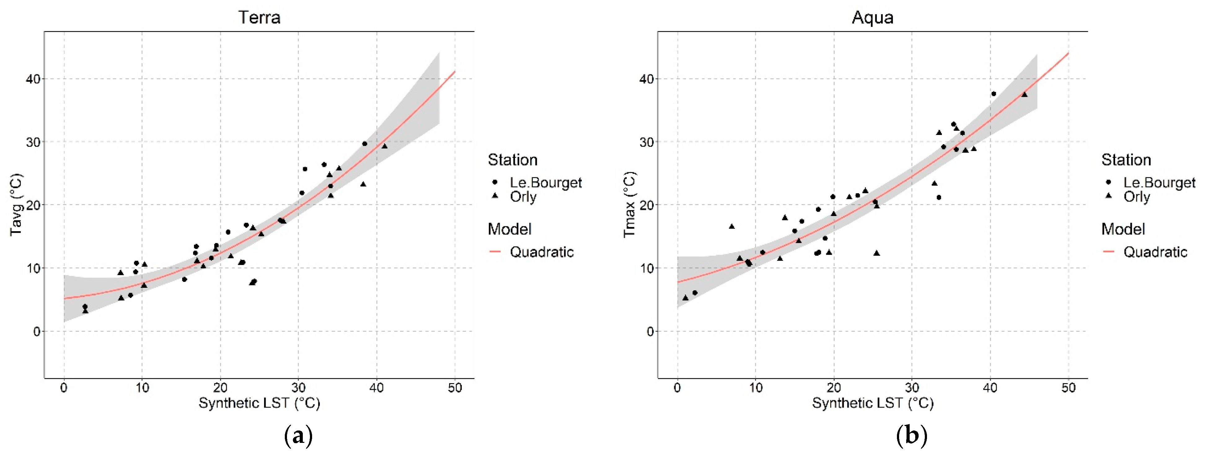
In this study, quadratic regression was used to calculate the relation between air temperature and synthetic LST using data from two weather stations in Paris, Le Bouget and Orly airport

3. Results

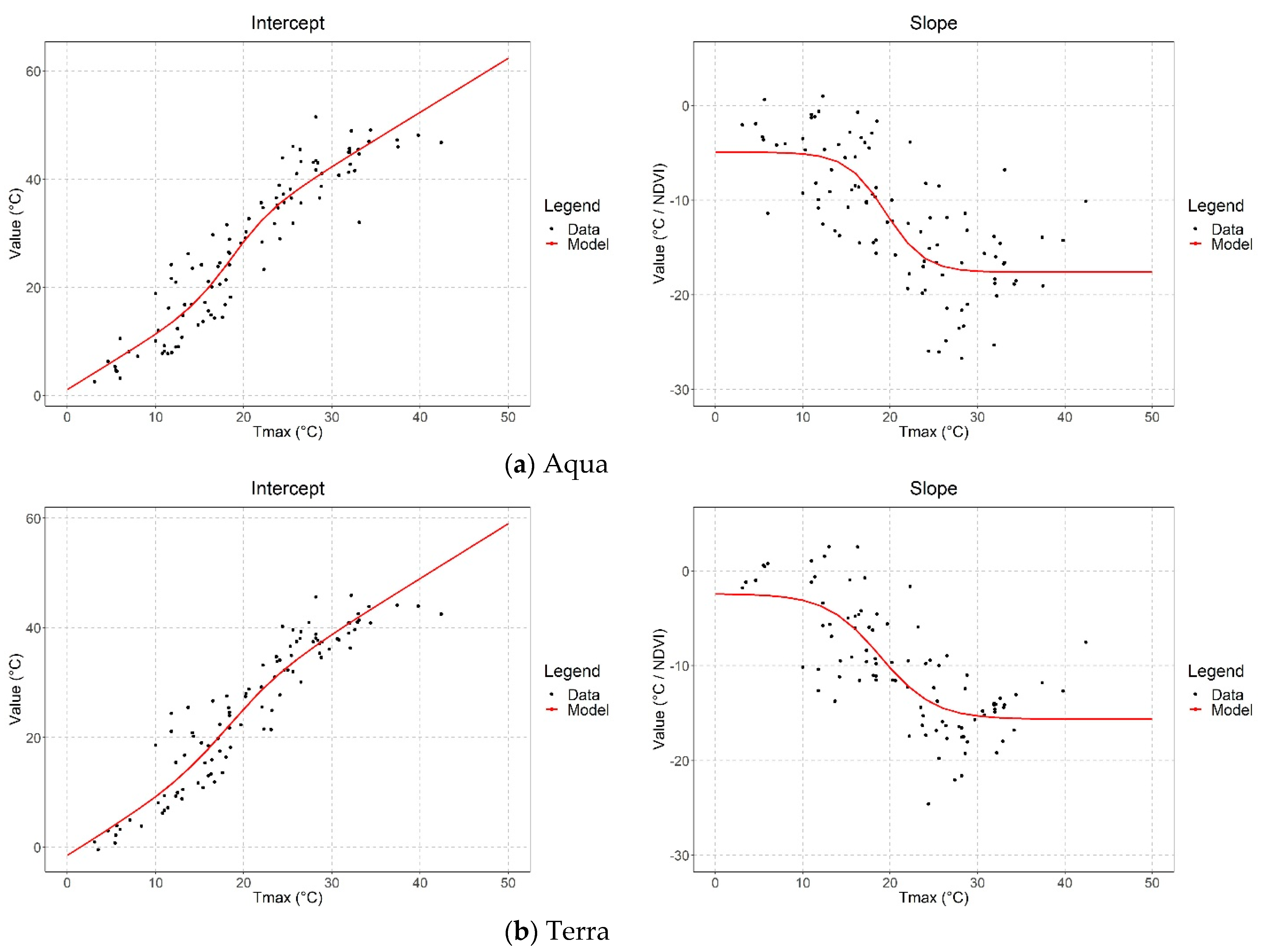
3.1. Temperature Variable DisTrad Parameters

The results from the first processing step are shown in Figure 5. Here one can see the variation in the intercept and slope as a function of maximum temperature throughout the year. The data suggests that a logistic function is more appropriate than a linear model for relating slope to temperature. The models used are:

$$\mathrm{Slope}={ \mathrm{a}}_{\mathrm{slope}}+\frac{{\mathrm{b}}_{\mathrm{slope}}}{\left(1-\exp (-{\mathrm{g}}_{\mathrm{slope}}* ({\mathrm{T}}_{\max }-{\mathrm{t}}_{\mathrm{slope}}\right)}$$

(2)

$$\mathrm{IIntercept}={ \mathrm{T}}_{\max }+{\mathrm{a}}_{\mathrm{intercept}}+\frac{{\mathrm{b}}_{\mathrm{intercept}}}{\left(1-\exp (-{\mathrm{g}}_{\mathrm{intercept}}* ({\mathrm{T}}_{\max }-{\mathrm{t}}_{\mathrm{intercept}}\right)}$$

(3)

The variables in the equations above are typical of logistic functions. The variable a controls the minimum of the curve. The sum of the variables a and b is the maximum of the curve. The variable g is the growth rate, and it controls how steep the transition between the curve’s minimum and maximum is. Finally, the variable t sets the inflection point of the curve.

Due to the difference in the time of the flyovers of the MODIS sensors (Aqua in mid-afternoon, Terra shortly after mid-day), the analysis proceeds separately for each sensor. For both the Aqua (

Table 1. Model parameters—Aqua.

Logistic Model
	a	b	t	g	R2	AIC
Intercept	1.14	11.2	18.6	0.434	0.883	606
Slope	−4.93	−12.7	19.5	0.449	0.563	586
Linear Model (c0 + c1 Tmax)
	c0	c1			R2	AIC
Intercept	−1.87	1.45			0.860	620
Slope	−0.592	−0.534			0.460	603

) and Terra (

Table 2. Model parameters—Terra.

Logistic Model
	a	b	t	g	R2	AIC
Intercept	−1.52	10.5	18.2	0.3145	0.869	613
Slope	−2.40	−13.2	18.8	0.326	0.585	538
Linear Model (c0 + c1 Tmax)
	c0	c1			R2	AIC
Intercept	−3.57	1.40			0.855	619
Slope	0.730	−0.513			0.490	554

) data, the r² is larger, and the Akaike information criterion (AIC) is smaller for a logistic model than for a simple linear regression. The lessening of the slope at lower temperatures is well known since at air temperatures below 10 °C photosynthesis decreases [25].

Above 30 °C, the relationship of photosynthesis with temperature is not straightforward. It is species-dependent and varies with water availability.

The logistic model suggests that there is a limit to the decrease of LST one can expect as a result of cooling by vegetation. The maximum magnitudes of the slope are 17.6, and 15.6 °C/NDVI, respectively, for Aqua and Terra data. With a maximum ΔNDVI of 0.7, these values mean that the maximum decrease in LST is 12.3 and 10.9 °C in mid-afternoon (Aqua) and midday (Terra).

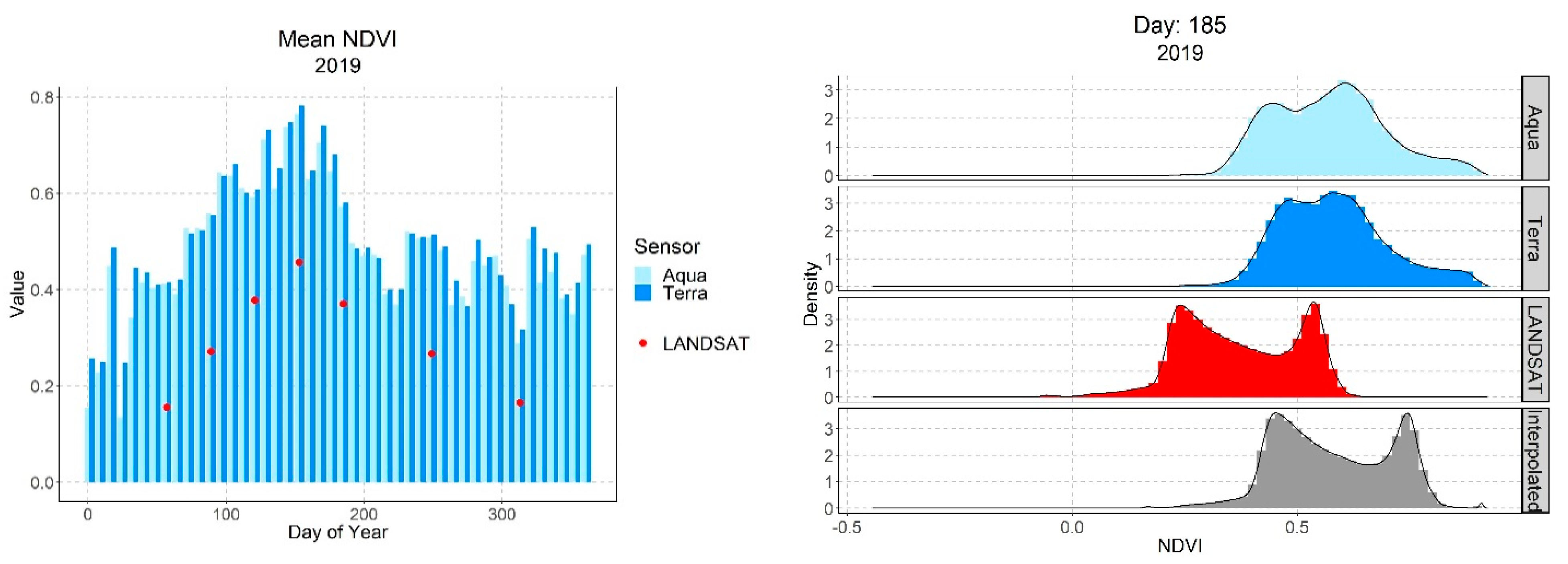
3.2. Interpolation of NDVI

Once the temperature variant DisTrad equation parameters have been calculated, they can be used in combination with a high resolution LANDSAT NDVI to create a simple DisTrad LST product. However, the availability of LANDSAT NDVI has the same constraints as the LANDSAT LST, namely, low temporal resolution (every 16-days) and losses due to clouds. To overcome these problems, one could naively propose simple linear interpolation between two good LANDSAT NDVI products as the buildings (lower NDVI) and green spaces (higher NDVI) do not move spatially. However, NDVI is known to be sensitive to rainfall in dry climates [26,27], and ground-based NDVI is sensitive to leaf and canopy properties [28]. In addition, the NDVI used in the DisTrad equations is from MODIS and not LANDSAT, which we use here. A comparison of the mean NDVI throughout the year for the various products is shown in Figure 6 (left). There is a monthly variation due to leaf and canopy properties, an inter-day variation presumably due to changes in rainfall, and even an intra-day variation. The NDVI from Terra (midday) is usually greater than the estimate from Aqua (mid-afternoon). In addition, the mean NDVI from LANDSAT (30 m × 30 m resolution) is much lower than the MODIS products (1000 m × 1000 m resolution). Hence, simple linear interpolation of LANDSAT NDVI alone is not adequate.

To correct this difference, after the linear interpolation of the LANDSAT NDVI, the resultant product is scaled so that its mean value equals the mean of the MODIS NDVI product for the day and time (i.e., Aqua or Terra) of interest. A comparison of the density plots for the three sensors and the interpolated NDVI is shown in Figure 6 (right).

It is important to note here, that the absolute value of the NDVI is not as important as the range of NDVI to the synthetic LST (output of step 3) due to the spatial filtering and combination step that follows. The high spatial frequency information from the DisTrad LST is used in synthetic LST; the low spatial frequency information (including the mean value) comes from the MODIS LST products themselves. The scaling of the interpolated NDVI allows for the comparison of the intermediate DisTrad product, to the LANDSAT LST.

3.3. Spatial Power Spectra of LANDSAT, MODIS and Simple DisTrad LST

A north-south transect through the three LST products (LANDSAT, simple DisTrad, and Terra) and the equivalent spatial power spectra are shown in Figure 7. Visual inspection of the transects shows that the DisTrad product lacks the low spatial frequency features of the LANDSAT LST, and the Terra LST is mostly devoid of high spatial frequency detail.

This observation is supported by the spatial power spectra. At low spatial frequencies (<0.000125 m⁻¹), the Terra spectrum is comparable to the LANDSAT spectrum. Above this spatial frequency, the simple DisTrad spectrum is more similar to the LANDSAT spectrum. At spatial frequencies above 0.0025 m⁻¹, the simple DisTrad has more power than the LANDSAT spectrum. This suggests the sum of products at different spatial bandwidths may provide a good estimate of the LANDSAT.

As introduced in the methodology section, the sum of low-pass filtered Terra LST and high-pass filtered simple DisTrad is used to model the LANDSAT LST. Filtering is performed using a circular, even weighted, average of a user specified radius. The same filter is applied to the Terra and simple DisTrad products as a low-pass filter. The low-pass filtered simple DisTrad product is subtracted from the DisTrad LST to create a high-pass filtered version. The two filtered sub-products are then summed to form the intermediary product. The choice of filter radius can be optimized to minimize the RMSE to the LANDSAT LST. The optimum filter length was tested and for these data occurs at 2000 m, as shown in Figure 8.

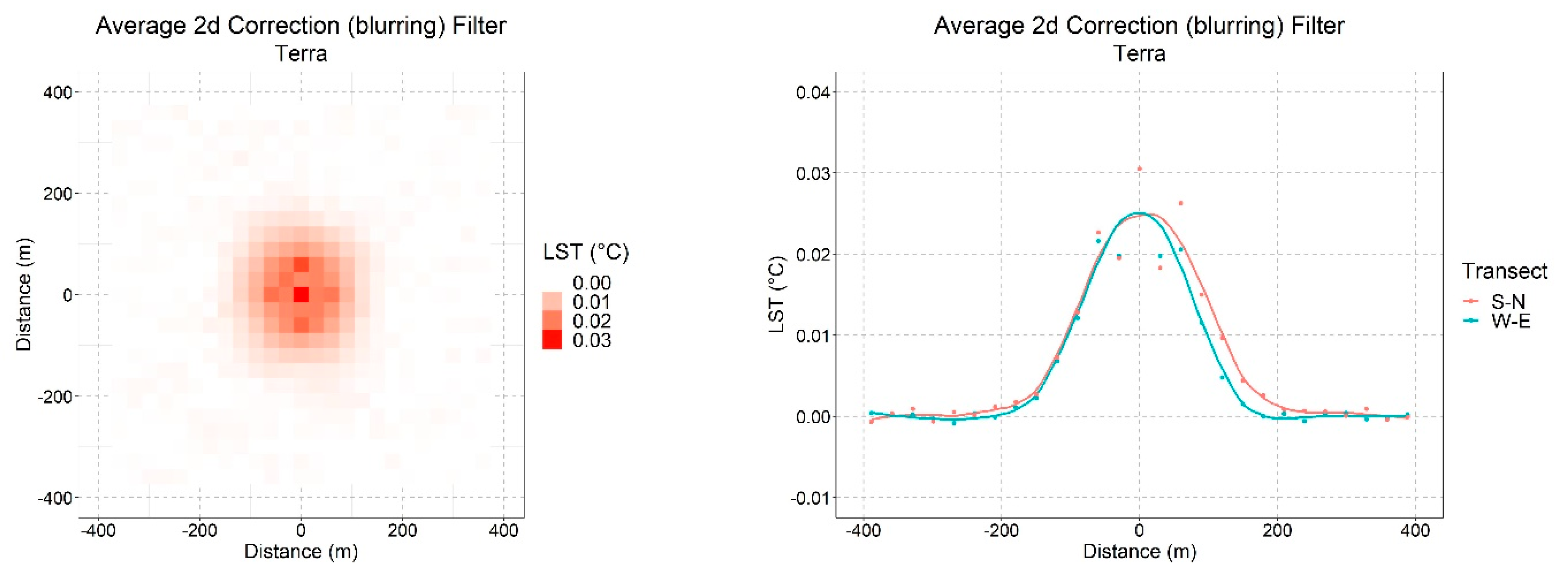
The final process in step 3 is the calculation of a correction (blurring filter). It is shown in Figure 9. It has the effect of spreading the heat at the center to ±200 m. The filter is not perfectly symmetric in that it is slightly broader to the north side. The sum of all points in the filter is unity, so it does not change the overall level of the scene.

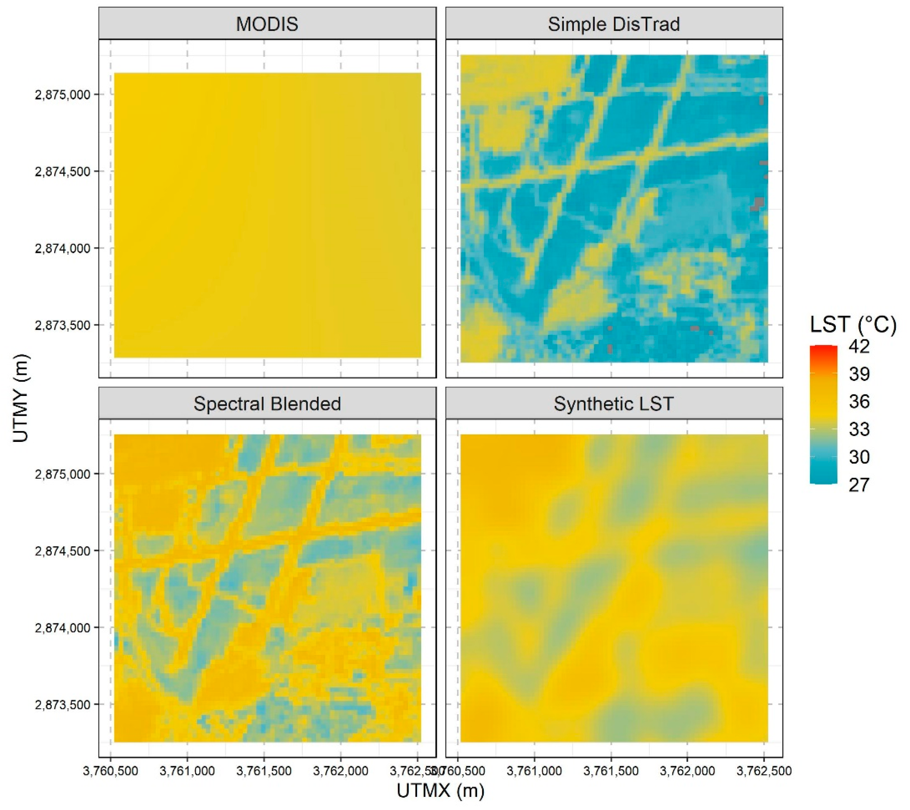
A visual summary of the processing steps to create the synthetic LST and a comparison to the LANDSAT LST is shown in Figure 10. The location is Orly Airport. The Terra LST (top left) is uniform over the small area shown in the scene. The simple DisTrad (top right) product shows sharp detail. The linear higher temperature features are the runways and the cooler areas in-between are grass. The synthetic LST (bottom right) shows the effect of the correction (blurring) filter, and it resembles the LANDSAT LST much better than the simple DisTrad.

A comparison of MSE, RMSE, and MAE after each of the processing steps is shown in

Table 3. Evolution of the mean squared error (MSE), root mean squared error (RMSE) and mean absolute error (MAE) during the processing steps. The “adjusted” indicators are used to remove the bias caused by differences in time of day.

Product	Mean [°C]	Adj. Mean [°C]	MSE [°C]	RMSE [°C]	Adj. MSE [°C]	Adj. RMSE [°C]	MAE [°C]	Adj. MAE [°C]
LANDSAT	27.7	27.7
MODIS Terra	28.3	27.7	7.1	2.7	6.8	2.6	2.1	2.0
DisTrad	28.7	27.7	7.8	2.8	7.0	2.6	2.3	2.1
Spatial bandwidth composition	28.3	27.7	5.7	2.4	5.4	2.3	1.9	1.8
Blurring filter	28.3	27.7	4.8	2.2	4.5	2.1	1.8	1.7

. There is a 15% improvement in RMSE from the spatial bandwidth composition process and a further 7% improvement from applying the blurring filter. The improvements are larger when the data are corrected for the bias caused by the difference in time of day.

The mean absolute error (MAE) is significantly less than the RMSE. This indicates that outliers are present in the products. Inspection of the entire LANDSAT image shows some very hot isolated locations (e.g., Stellantis automotive factory in Poissy: 48.937 N, 2.044 E, 51.6 °C). This location is not shown in Figure 10. Another source of outliers is water bodies, as they have negative NDVI and would appear as very cold spots using a DisTrad-based methodology unless the calculated NDVI is replaced by some value. Water bodies are not modeled properly using this method.

3.4. Converting LST to Air Temperature

With the ability to produce a synthetic LST image for every day in the year, one can build a linear relationship between the synthetic LST (either Terra or Aqua-based) to a temperature indicator (e.g., average or maximum) from one or more weather stations [14,15,16,18,19]. However, non-linear relationships have also been modeled [13,17], especially for higher temperatures. Here the relationship is modeled as a quadratic function. Figure 11 displays these relationships for modeled air temperature against measured air temperature for the two weather stations in Paris with publicly available data, Le Bouget and Orly airport. The regression parameters are shown in

Table 4. Model parameters—T_avg and T_max as second order polynomial function of synthetic LST.

Indicator	Product	Intercept	Linear-Term	Quadratic-Term	R2
Tavg	Terra	5.18	0.120	0.0120	0.854
Tmax	Aqua	7.76	0.310	0.00834	0.862

.

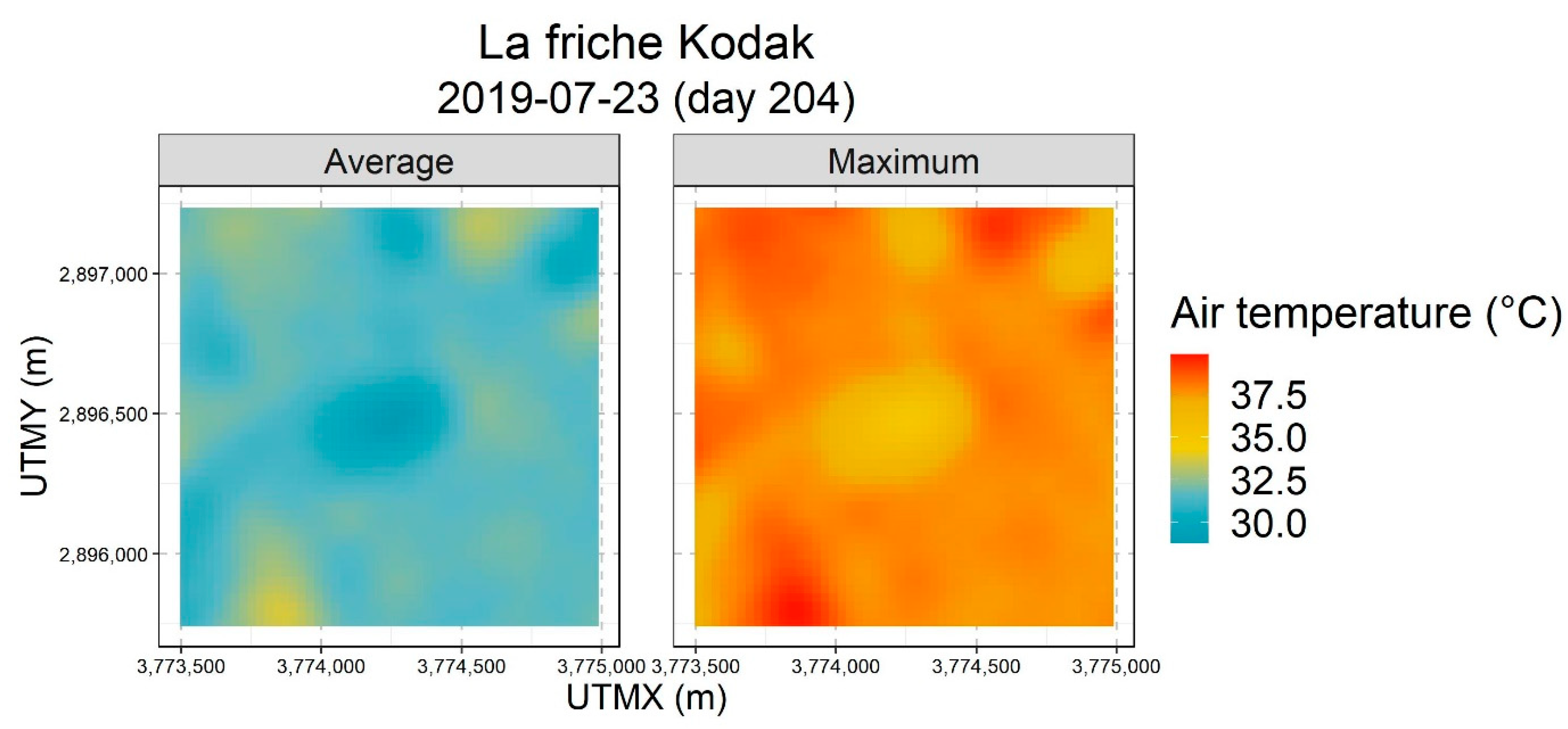
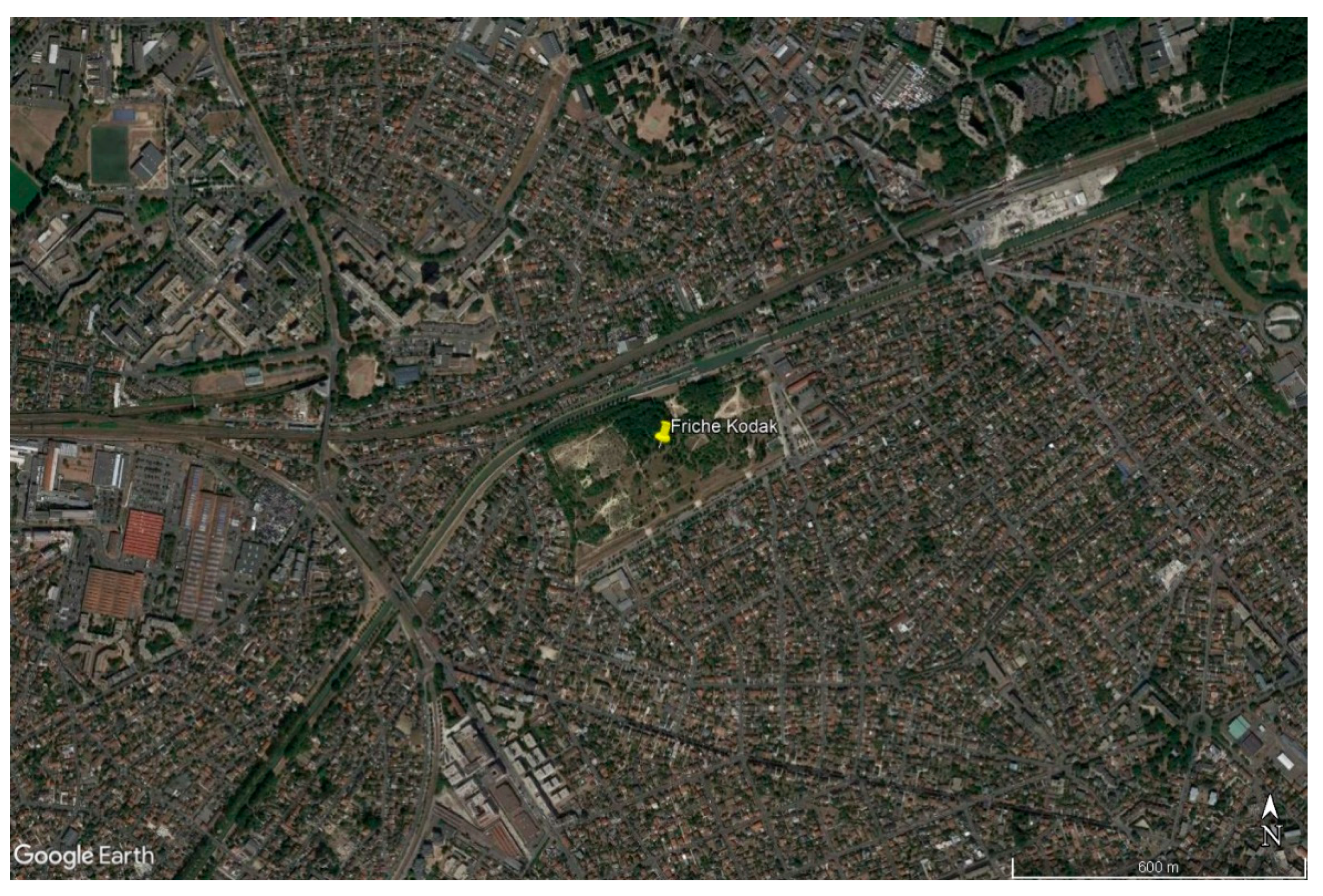
With these relationships, one can transform the LST into modeled average and maximum air temperature products. Figure 12 shows these products in detail for a small park. At the center of the scene is La friche Kodak, a 14 ha denaturalized area recovered from the former Kodak Industrial Site. The park is 270 m × 480 m of mixed grassland and trees. NDVI (not shown) in the park has a maximum value of 0.57 and an average value of 0.40 as compared to the surrounding built-up area (0.25). The scene selected (23 July) was the hottest day of the year in 2019. The modeled average air temperature in the park center is 28.9 °C, about 2.3 °C cooler than the surroundings. The modeled maximum temperature in the park center is 35.0 °C, which is 3.1 °C cooler than the surroundings (38.1 °C). A Google Earth Image of La friche Kodak is provided for reference (Figure 13).

4. Discussion

4.1. Temperature Variable DisTrad Functions

The relationship of the DisTrad slope with temperature showed a good fit with the logistic curve model at low temperatures. However, on days with the highest temperatures, the fit was not as good, and the absolute value of the DisTrad slope was well below the fitted line in some cases. This suggests that there are other factors influencing the ability of vegetation to provide cooling (i.e., actual DisTrad slope less than the modeled curve).

Studies of stomatal conductance indicate that if there is sufficient water, then higher temperatures lead to higher stomatal conductance and hence higher photosynthesis [29,30]. Many studies conclude that drought is more significant than heat as a stressor for plant dynamics [31,32,33,34]. A decrease in photosynthesis in Mediterranean Oaks has been observed above an air temperature of 30 °C [35] and above 40 °C in oaks in Western USA [36], but these authors did not consider the influence of drought.

Hence, a combination of high temperatures and prolonged dry periods may explain the low DisTrad slopes on some days in this study. The overall response of the DisTrad slope to drought and temperature will not be simple, because Paris is in an area with strong human influence. Some green areas may be irrigated, and others not. In addition, as the drought continues in the extreme, irrigation will be discontinued. If this is the case, in prolonged dry periods, the DisTrad slope versus temperature may not be a logistic curve, but starts decreasing at high temperatures, due to the loss of evapotranspirative cooling under drought conditions. In arid climates, studies of LST and vegetation have documented that there may be little to no cooling from vegetation [37,38,39,40].

4.2. Spatial Bandwidth Limited Mixing of MODIS and Simple DisTrad Products

The optimal spatial filter radius of 2000 m is double the spatial resolution of the MODIS LST. This is probably not a coincidence. The Nyquist frequency for something sampled every Δx m is 1/(2 Δx) and does not include information at frequencies above this value (if properly sampled). The boxcar filter with a length of 2 L has a frequency notch at 1/(2 L). In this study, the smoothing filter (a circular boxcar filter) has a radius of 2000 m (L), and the notch occurs at the Nyquist frequency. Since the RMSE is dominated by low spatial wavelengths, the optimal filter radius should always be around 2000 m.

In “R”, the platform used to process these data, the spatial filtering program “focal” requires that within the filter area all values exist (i.e., non-NA), or an NA value is returned. This means that NA values in all products should be filled since the spatial bandwidth mixing step applies a large spatial filter (r = 2000 m) to both the MODIS and the simple DisTrad product. The issue of the size of filters is not limited to NA values, however. Studies that include large bodies of water (i.e., ocean or large lakes) or large mountains may require special processing so that unwanted edge effects during the application of the filters are minimized. Such geographical effects do not affect the study region in this paper.

4.3. Correction (Blurring) Filter

The correction (blurring) filter size of 200 m is an interesting observation. The filter is required to blur the composite LST based on LANDSAT resolution (30 m × 30 m) NDVI to be more like the LANDSAT LST. The value we report here is data-driven, i.e., that relationship has emerged from the data. A possibility is that different remote sensors cause it. However, as the high spatial frequency component of the composite LST and the LANDSAT LST are both from the same sensor, one would think that different sensors would not likely be the cause.

Another possibility is that the correction (blurring) filter is a natural outcome of the mixing of air between cooler and warmer locations—i.e., it represents the effectiveness of green spaces in cooling surrounding areas. Studies of air temperature profiles moving away from parks have found curves similar to the negative of the blurring filter. The distance of measured cooling may vary depending on park size. Yu et al. (2017) found cooling extending to a distance of 60 to 280 m in Fuzhou, China [41]. Sugawara et al. [42] measured a distance of about 200 m and an impact of wind direction. Other authors have estimated the distance to be about 300 m [3,43], and Doick, Peace, and Hutchings [44] found the nighttime effects of Kensington Gardens in London, England, to extend between 20 and 440 m away from the park boundary depending on weather conditions.

The application of the correction (blurring) filter has significant implications for designing strategies to adapt to increased urban warming using nature based solutions (NBS): (1) individual trees and pocket parks will have little impact on air temperature unless they are uniformly spaced throughout the city, and (2) the full cooling impact of an NBS is reached only if a park is more than 200 m wide. These concepts are discussed in detail by Yue et al. [45].

4.4. Air Temperature Versus LST

Air temperature and LST represent outcomes of slightly different physical processes. They respond differently to atmospheric, hydrological, and ecological conditions [46,47]. In addition, the emissivity of the surfaces strongly influences the relationship [48]. Many methods have been developed to estimate air temperature from MODIS LST [47,49,50,51] and inconsistencies over large distances have been documented mostly due to elevation effects [17]. In this study, because we are using LST based on a mixed LANDSAT, MODIS product, we have opted to use a simple regression to known weather stations within the study area as these data are used for input to other studies [5,52,53]. This method, although simple, has problems if one wants absolute (and not relative) air temperature over the entire city. However, LST is known to have variation beyond a simple relationship to NDVI in cropland, water bodies, and snowy landscapes and is also influenced by elevation or topography. Weather stations measure temperature in a standardized, systematic manner, but this does not include understory air temperature.

Despite the strong linear relationship between LST and air temperature found in this study, there may be spatially varying effects in either the air temperature or LST data. In this situation, a simple linear regression over many weather stations may not be suitable to resolve this with sufficient accuracy. A more appropriate method to convert LST to air temperature may be co-kriging [54], a method used predominantly in geological geospatial analysis [55,56]. However, for only two weather stations, as in this example, this approach is not possible.

4.5. Limitations

The methodology described in this paper has some limitations. In the interim product, the low spatial frequency LST is corrected for high spatial frequency NDVI vegetation effects only. Because the method uses MODIS LST as its basis, low spatial frequency features such as the gradual increasing density of built up areas, changes in building heights and materials by district, or district scale topographic effects should be incorporated. However, local scale impacts of building materials (e.g., cement versus asphalt parking lot), different albedo (e.g., a building with white versus dark façades), and local wind, humidity, and shadow effects, and point sources of heat (e.g., air conditioning cooling vanes, heavy industry) are not included. Some of this variation may be addressed if the regression (in step 2) includes more predictors. This has been tested by Liu et al. [19].

In addition, one should remember that air temperature is related to, but not exactly what, people experience. For studies on human exposure, an indicator, such as the Physiological Equivalent Temperature index [57], is more appropriate.

5. Conclusions

In this paper, a methodology is presented whose goal is to produce a spatially continuous proxy for weather station air temperature using freely available data such as LANDSAT and MODIS remote sensing products and weather station temperature records, for example, from NOAA or the national weather service. This goal is accomplished in two steps. Firstly, a variation of the DisTrad method is presented that mixes high spatial resolution, and vegetation related LST impacts, using the normalized differential vegetation index (NDVI) from LANDSAT with lower spatial frequency and resolution background LST from MODIS in different spatial-frequency bands (spatial spectral composition) to provide high-resolution LST. A blurring filter that may be a result of heat dissipation then further modifies this product. The method allows for the calculation of high-resolution LST two times daily on any day of the year. The two times during the day depend on the flyover times of the MODIS Terra and Aqua sensors. Secondly, the daily high-resolution LSTs that result from the first step are used to define a transfer function to convert Terra and Aqua-based products to average and maximum daily air temperatures under the assumption of ergodicity.

An example of the use of this methodology is applied in Paris, Île de France. It is shown that the methodology relatively accurately replicates the LANDSAT LST (RMSE = 2.1 °C, MAE = 1.7 °C). On 23 July 2019, the methodology models that a small park, La friche Kodak, was 2.3 °C cooler at midday and 3.1 °C cooler in mid-afternoon than the surrounding urban area.

The availability of a spatially continuous proxy for weather station air temperature component on multiple days, that includes influences of NBS, would be extremely helpful in studies investigating temperature influences at a fine scale, for example, in cities, when looking at human mortality and health, or energy demand for heating and cooling. These studies may be used to calculate the economic benefits of NBS. In addition, a detailed analysis of the products could be used to identify the optimal design of NBS (size, shape, maximum NDVI attained), and spacing of NBS within the urban landscape. The optimal design could be used as input to forward thinking studies on adaptation to climate change.