Atmospheric Gravity Wave Potential Energy Observed by Rayleigh Lidar above Jiuquan (40° N, 95° E), China

Abstract

Two years of observational data from the 532 nm Rayleigh lidar were used to study the vertical profile characteristics of atmospheric gravity wave potential energy density (GWPED) between 40–80 km above Jiuquan (40° N, 95° E) for the first time. The atmospheric gravity waves (AGWs) characteristics are presented in terms of the atmospheric relative temperature perturbation, along with the estimated annual and seasonal GWPED with high spatial and temporal resolution (0.5 km and 1 h). The annual potential energy mass density ${\mathrm{E}}_{\mathrm{pm}}$ and volume density ${\mathrm{E}}_{\mathrm{pv}}$ vertical profiles show that the GWPED in the upper mesosphere is close to the adiabatic growth rate. The seasonal vertical profiles result shows that ${\mathrm{E}}_{\mathrm{pm}}$ is higher in autumn–winter than in spring–summer in all the observed altitudes. The GWPED approaches adiabatic growth above 61 and 65 km in spring–summer and autumn–winter, respectively. The AGWs severely dissipate below the turning altitudes and transfer energy into the background atmosphere. The GWPED scale heights show that the AGWs dissipation rate of spring–summer is close to that of autumn–winter. Furthermore, based on the wind data from SD–WACCM, the influence of critical level filtering on AGWs is discussed. It plays an important role in affecting the seasonal variation in GWPED.

1. Introduction

Atmospheric gravity waves (AGWs) are an important dynamic process in the middle atmosphere, and they are a key factor affecting atmospheric circulation, thermal structure distribution, and chemical component transport [1]. In the middle atmosphere, the typical scale of AGWs is tens to a few thousands of kilometers in horizontal wavelength and several to tens of kilometers in vertical wavelength [2]. In current general circulation models (GCMs) and chemistry climate models (CCMs), the influence of AGWs activity is the main source of model uncertainty. Therefore, to improve and tune AGWs parameterizations in models, more studies are needed to reveal the characteristics of AGWs.

Gravity wave potential energy density (GWPED) is considered a critical measure of the strength of AGWs activities [3,4], which can be utilized to derive the momentum flux, an important parameter for the observation as well as parameterization of AGWs. Lidar has the advantages of high temporal resolution, high spatial resolution, and continuous observation, which can be used to study GWPED. The rotational Raman lidar and metal fluorescence lidars are used for measurement in the lower atmosphere and mesosphere and lower thermosphere (MLT), respectively [5,6,7,8]. For the main dissipation region of AGWs (stratosphere and mesosphere), Rayleigh lidar is widely used in measurement. Wilson et al. [9] performed a detailed study of AGWs between 30 and 75 km altitudes with Rayleigh lidar from two stations at 40° N in southern France, and compared the seasonal profiles and daily mean variation characteristics on GWPED. In the study of AGWs between 35 and 50 km above Toronto (44° N, 80° W), Whiteway and Carswell [10] found the same seasonal variation characteristics as the study in the south of France, with maximum mass potential energy density ${\mathrm{E}}_{\mathrm{pm}}$ in the winter and minimum in the summer. Sivakumar et al. [11] studied the AGWs between 30 and 70 km above Gadanki (13.5° N, 79.2° E) and found that the ${\mathrm{E}}_{\mathrm{pm}}$ is higher in the low-latitude regions than in the mid-latitude regions. Thurairajah et al. [12] studied Alaska’s (65° N, 147° W) AGWs between 40 and 80 km for three winters and found that the average ${\mathrm{E}}_{\mathrm{pm}}$ is ~2.6 J/kg, which is less than that of the mid-latitudes. Kafle [13] researched the seasonal variation in the GWPED between 45 and 90 km above Logan, Utah (41.74° N, 111.81° W), and showed that the GWPED has significant daily and seasonal variations. Mzé et al. [14] pointed out that ${\mathrm{E}}_{\mathrm{pm}}$ peaks in winter and noted the minimum in summer in the upper stratosphere (30–50 km) from the vertical distribution of the GWPED between 30 and 85 km above Haute-Provence Observatory (43.93° N, 5.71° E). The lower mesosphere also has a maximum in winter. However, in the upper mesosphere, the maximum AGWs activity occurs in winter and summer. Guo et al. [15] studied AGWs between 30 and 70 km above Beijing (40° N, 116° E) and showed that the ${\mathrm{E}}_{\mathrm{pm}}$ varies with seasons and altitudes, and the AGWs activity intensity during winter is about twice that of summer. Chen [16] studied AGWs between 30 and 55 km above Wuhan (31° N, 114° E) and showed that the statistical results in this area are basically consistent with other mid-latitude regions and that the average ${\mathrm{E}}_{\mathrm{pm}}$ in winter is twice the average ${\mathrm{E}}_{\mathrm{pm}}$ in summer. These studies demonstrate the reliability of Rayleigh lidar applied to the study of AGWs and reveal the GWPED characteristics of the stations at different geographic locations.

A recent observational dataset was collected above Jiuquan (40° N, 96° E) during 2019–2020 based on the Rayleigh lidar, which can be used to investigate GWPED. Jiuquan is located in the northern foothills of the Qinghai–Tibet Plateau, the third pole of the world. A total of 471 h of temperature profiles through temperature perturbations were used to investigate GWPED characteristics between 40 and 80 km above Jiuquan. Section 2 gives the data and methods of analysis. Section 3 shows the results. The conclusions and discussion are presented in Section 4 and Section 5, respectively.

2. Data and Analysis Methods

2.1. Rayleigh Lidar and Data

The 532 nm Rayleigh lidar used in this study was initially developed in 2014 and routinely operated [17]. During 2019–2020, the lidar moved to Jiuquan. It provided stratospheric and mesospheric hourly-mean nocturnal temperature measurements, from which the relative density profiles were normalized to absolute density values at 35 km altitude from the NRLMSIS–00 to produce the absolute density profiles. The density and temperature data used in this study have a temporal resolution of 1 h and a spatial resolution of 0.5 km. The main performance parameters of the lidar are shown in

Table 1. Main parameters of the Rayleigh lidar.

Parameters	Value
Laser Wavelength/nm	532
Laser Power/W	15
Pulse Repeat Frequency/Hz	30
Pulse Duration/ns	7
Telescope Aperture/cm	100
Bandwidth of Interference filter/nm	1.0

.

Excluding the nocturnal lidar observation data with a continuous observation time of less than 5 h, a total of 55 days (471 h) of data were acquired. The average daily observation time was 8.6 h. The temporal distribution data are shown in

Table 2. Statistics of the temperature data.

2019	April	May	November	December	Total
Observations/days	3	5	10	6	24
Observation hours/h	22	32	83	53	190
2020	May	Jun	Nov		Total
Observations/days	11	4	16		31
Observation hours/h	79	32	170		281

and divided into two parts: the Spring–Summer part for April, May, and June; and the Autumn–Winter part for November and December.

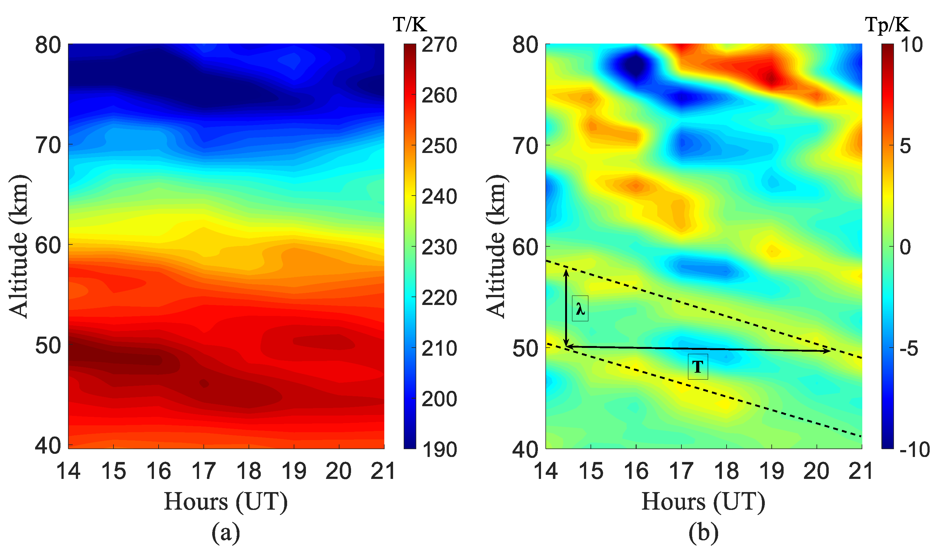
2.2. Extraction Method of Temperature Perturbations

The algorithm below details the temperature perturbations extraction method used by Gardner [18]:

• Eliminate the temperature data with uncertainty higher than 10 K to retain the data with higher reliability.
• Fit a straight line to the temperature temporal series for each altitude during the nocturnal observation to obtain the background temperature.
• Obtain the temperature perturbation ${\mathrm{T}}^{\prime }\left(\mathrm{z}\right)$ by subtracting the background temperature from the measured temperature.

As the time duration of each night data on average is 8.6 h and the time interval is 1 h, temperature perturbations are mainly caused by AGWs. The characteristics of AGWs with a period of 2 h from the observation duration the night can be obtained from this data.

The background temperature obtained by this method includes the trend in atmospheric temperature as a function of time. Subtracting the background temperature can effectively eliminate the influence of long-period waves, such as tidal, planetary, and gravity waves, whose periods exceed the observation period. The GWPED is slightly higher using the above method than the considerate method between 84 and 100 km, which can remove the real background based on the full-diurnal-cycle observations [7]. Below 80 km, the tides’ amplitudes decrease a lot versus decreasing height, especially below 70 km, where they are too small and should be neglected compared with AGWs activities.

For example, the nightly temperature contour plot for the temperature data from 10 May, 2020 is shown in Figure 1. Figure 1a shows the continuous 8 h observation data from 14:00 UT to 21:00 UT, where the temperature ranges from ~255.7 K at 40 km to ~197.1 K at 80 km, and the temperature uncertainty is ~0.2 K at 40 km and increases to ~3.6 K at 80 km. The stratopause is clear at ~50 km. Figure 1b shows the AGWs-induced temperature perturbations. The downward phase progression is clearly seen, which suggests a dominant quasi-monochromatic inertial gravity wave with an apparent period of ~6 h and vertical wavelength of ~8 km, which can be roughly estimated using the data below 60 km, as indicated by the dashed line in Figure 1b.

2.3. Calculation of GWPED and Scale Height

GWPED measures the strength of AGWs. The mass density ${\mathrm{E}}_{\mathrm{pm}}$ is the measure of wave amplitude, and the volume density ${\mathrm{E}}_{\mathrm{pv}}$ can be used to measure the degree of dissipation of AGWs. The calculations of ${\mathrm{E}}_{\mathrm{pm}}$ and ${\mathrm{E}}_{\mathrm{pv}}$ are shown in Equations (1) and (2) [3,9]:

$${\mathrm{E}}_{\mathrm{pm}}\mathrm{z}=\frac{1}{2}\frac{{\mathrm{g}}^2}{{\mathrm{N}}^2\mathrm{z}}{\left(\frac{ {\mathrm{T}}^{\prime }\left(\mathrm{z}\right)}{{\mathrm{T}}_0\left(\mathrm{z}\right)}\right)}^2$$

(1)

$${\mathrm{E}}_{\mathrm{pv}}\mathrm{z}={\mathsf{\rho }}_0\left(\mathrm{z}\right){\mathrm{E}}_{\mathrm{pm}}\left(\mathrm{z}\right)$$

(2)

where the gravitational acceleration g is 9.7 m/s²; ${\mathrm{T}}^{\prime }$ is the temperature perturbation; ${\mathrm{T}}_0$ is the background temperature, estimated as the average of the measured temperature over the observation nocturnal time here for simplified calculation; ${\mathsf{\rho }}_0\left(\mathrm{z}\right)$ is the background density, which is the profile obtained by the averaged density at each height during the night; and ${\mathrm{N}}^2$ is the square of the Brunt–Väisälä frequency given by [19]:

$${\mathrm{N}}^2\mathrm{z}=\frac{\mathrm{g}}{{\mathrm{T}}_0}\left(\frac{{\mathrm{dT}}_0\left(\mathrm{z}\right)}{\mathrm{dz}}+\frac{\mathrm{g}}{{\mathrm{C}}_{\mathrm{p}}}\right)$$

(3)

where ${\mathrm{dT}}_0\left(\mathrm{z}\right)/\mathrm{dz}$ is the mean temperature gradient, and ${\mathrm{C}}_{\mathrm{p}}$ = 1004 J/K/kg is the specific heat of dry air at constant pressure. The uncertainty associated with ${\mathrm{E}}_{\mathrm{pm}}$ and ${\mathsf{\sigma }\mathrm{E}}_{\mathrm{pm}}$ is calculated as follows:

$${\mathsf{\sigma }}^2{\mathrm{E}}_{\mathrm{pm}}={\left(\frac{\partial {\mathrm{E}}_{\mathrm{pm}}}{\partial {\mathrm{T}}^{\prime }}\right)}^2{\mathsf{\sigma }}^2 {\mathrm{T}}^{\prime }+{\left(\frac{\partial {\mathrm{E}}_{\mathrm{pm}}}{\partial {\mathrm{N}}^2}\right)}^2{\mathsf{\sigma }}^2{\mathrm{N}}^2+{\left(\frac{\partial {\mathrm{E}}_{\mathrm{pm}}}{\partial {\mathrm{T}}_0}\right)}^2{\mathsf{\sigma }}^2{\mathrm{T}}_0$$

(4)

Compared with the magnitude order of ${\mathrm{E}}_{\mathrm{pm}}$, ${\mathsf{\sigma }}^2{\mathrm{E}}_{\mathrm{pm}}$ is not significant. ${\mathrm{E}}_{\mathrm{pm}}$ can be precisely estimated when using multiple profiles and sufficient data. Therefore, the uncertainty associated with ${\mathrm{E}}_{\mathrm{pm}}$ was ignored. Similarly, the uncertainty of ${\mathrm{E}}_{\mathrm{pv}}$ is no longer considered.

The atmospheric density scale height is calculated as follows:

$$\mathrm{H}=-{\left(\frac{\mathrm{dln}\mathsf{\rho }}{\mathrm{dz}}\right)}^{-1}$$

(5)

For an upward-propagating AGW, its amplitude exponentially increases versus increasing height due to the exponentially decreasing atmospheric density according to the non-dissipating linear gravity waves theory. For the energy conserved (non-dissipated) AGWs, ${\mathrm{E}}_{\mathrm{pv}}\mathrm{z}$ stays constant versus increasing height, while ${\mathrm{E}}_{\mathrm{pm}}$ exponentially grows with the atmospheric density scale height of H or the adiabatic growth rate of 1/H.

It is well-known that upward-propagating AGWs are filtered by critical levels in the stratosphere, which become broken and saturated in the upper mesosphere due to their amplitudes increasing too much. These processes cause the AGWs to dissipate while propagating upward through the atmosphere. If the linear propagation cases are considered, the main reason for the ${\mathrm{E}}_{\mathrm{pm}}$’s scale height deviation from H means that dissipation occurs and transfers energy into the background atmosphere.

In order to better understand AGWs dissipation by observing the potential energy density, we define the potential energy density scale height ${\mathrm{H}}_{\mathrm{pm}}$ and ${\mathrm{H}}_{\mathrm{pv}}$:

$${\mathrm{E}}_{\mathrm{pm}}\mathrm{z}={\mathrm{E}}_{\mathrm{pm}}{\mathrm{z}}_0\exp \left(\frac{\mathrm{z}-{\mathrm{z}}_0}{{\mathrm{H}}_{\mathrm{pm}}}\right)$$

(6)

$${\mathrm{E}}_{\mathrm{pv}}\mathrm{z}={\mathrm{E}}_{\mathrm{pv}}{\mathrm{z}}_0\exp \left(\frac{{\mathrm{z}}_0-\mathrm{z}}{{\mathrm{H}}_{\mathrm{pv}}}\right) .$$

(7)

According to this definition, these scale heights are indicators of the dissipation of gravity wave energy: when ${\mathrm{H}}_{\mathrm{pm}}$ is positive and larger than H, it means that the increase in ${\mathrm{E}}_{\mathrm{pm}}$ with altitudes is slower than the energy conservation wave, and the AGWs experience dissipates. The positive ${\mathrm{H}}_{\mathrm{pv}}$ means that the AGWs dissipate with increasing altitude. For energy conservation AGWs, ${\mathrm{H}}_{\mathrm{pv}}$ remains infinity with increasing altitude [8,20].

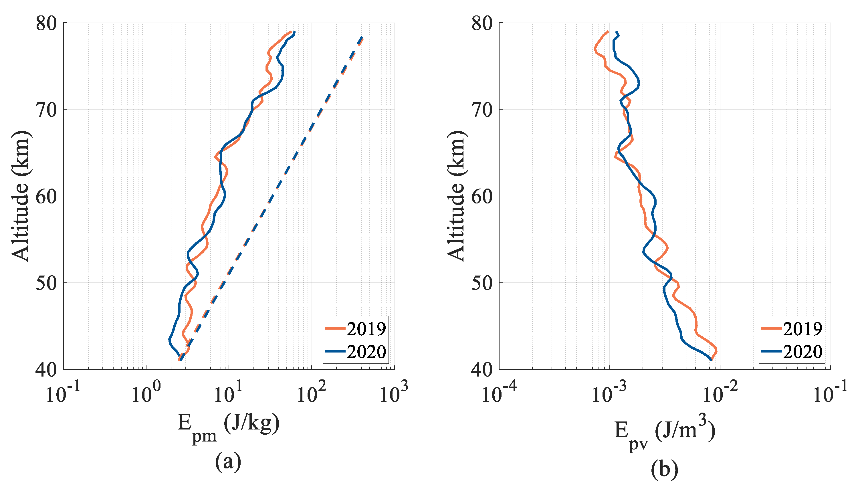
3. Results and Analysis of GWPED

According to the method above, the averaged GWPED profiles between 40–80 km above Jiuquan in 2019 and 2020 are shown in Figure 2. The two-year annual average GWPED profiles are close to each other, and the ${\mathrm{E}}_{\mathrm{pm}}$ shows an increasing trend with increasing altitude, while the ${\mathrm{E}}_{\mathrm{pv}}$ shows a decreasing trend. The dashed line in Figure 2a indicates the increasing trend for energy conservation AGWs.

In Figure 2a, the growth rate in ${\mathrm{E}}_{\mathrm{pm}}$ is close to the adiabatic growth rate above 65 km and less than the adiabatic growth rate below 65 km, which suggests that the AGWs are nearly energy conservative between 65 and 80 km and dissipated between 40 and 65 km. In Figure 2b, the ${\mathrm{E}}_{\mathrm{pv}}$ decreases from 40 to 65 km and becomes nearly constant above 65 km, which agrees with Figure 2a that the AGWs are closer to energy conservation in the upper mesosphere than in the stratosphere and lower mesosphere. The main dissipation process may be a stratospheric and lower mesospheric wind filter, which can account for the GWPED dissipation profiles below 65 km.

The seasonal distribution of the observation data is divided into two parts: spring–summer (April and May in 2019, May and June in 2020) and autumn–winter (November and December in 2019, November in 2020). Figure 3a shows the ${\mathrm{E}}_{\mathrm{pm}}$ and ${\mathrm{E}}_{\mathrm{pv}}$ profiles for different seasons. In Figure 3a, both ${\mathrm{E}}_{\mathrm{pm}}$ and ${\mathrm{E}}_{\mathrm{pv}}$ are higher in autumn–winter than in spring–summer. Like Figure 2, in autumn–winter, the growth rate of the ${\mathrm{E}}_{\mathrm{pm}}$ is close to (lower than) the adiabatic growth rate at the upper height (lower height). The difference is that the turning altitude is 65 km in autumn–winter and 61 km in spring–summer. The turning altitude in autumn–winter is higher than that in spring–summer. The ${\mathrm{E}}_{\mathrm{pv}}$ value in Figure 3b agrees with the above.

The AGWs dissipation in spring–summer and autumn–winter mainly occurs between 40 and 61 km and 40 and 65 km, respectively. Equations (6) and (7) were used to estimate the GWPED scale heights in the dissipation altitude ranges, and the fitted dashed line is shown in Figure 3. As shown in

Table 3. Scale heights (${\mathrm{H}}_{\mathrm{pm}}$, ${\mathrm{H}}_{\mathrm{pv}}$, and $\mathrm{H})$.

	Spring–Summer	Autumn–Winter
${\mathrm{H}}_{\mathrm{pm}}$ (km)	17.19	20.54
${\mathrm{H}}_{\mathrm{pv}}$ (km)	12.94	10.95
$\mathrm{H}$ (km)	7.38	7.14

, the estimated ${\mathrm{H}}_{\mathrm{pm}}$ in autumn–winter is slightly larger than that in spring–summer, and ${\mathrm{H}}_{\mathrm{pv}}$ in spring–summer is slightly greater than in autumn–winter, which means that the autumn–winter waves’ energy dissipation rate at 40–61 km is almost equal to that of spring–summer at 40–65 km. H, ${\mathrm{H}}_{\mathrm{pm}}$, and ${\mathrm{H}}_{\mathrm{pv}}$ are intrinsically related by Equations (5)–(7) as $1/{\mathrm{H}}_{\mathrm{pm}}+1/{\mathrm{H}}_{\mathrm{pv}}=1/\mathrm{H}$, which is consistent, as shown in Table 3.

4. Discussion

The data obtained by the 532 nm Rayleigh lidar indicate that the ${\mathrm{E}}_{\mathrm{pm}}$ above Jiuquan is higher in autumn–winter than in spring–summer. Their energy dissipation rates in the stratosphere and lower mesosphere are similar, as well as in the upper mesosphere below 80 km. The AGWs act as energy-conservation AGWs, which agree with previous results [8,9,13,15].

The NCAR Community Earth System Model (CESM) includes an atmospheric model that extends in altitude to the lower thermosphere, which is known as the Whole Atmosphere Community Climate Model (WACCM). Because wind filtering is the main reason for AGWs dissipation in the stratosphere and mesosphere [9,21], WACCM was run in the specified dynamics mode (SD–WACCM) to output the wind profiles below 80 km. SD–WACCM demonstrates its reliability by integrating dynamic parameters from observational or reanalysis data [22,23]. The dataset was used to interpolate the wind with the hours of the lidar observations above Jiuquan. The interpolated wind profiles were averaged to obtain the background wind profiles for spring–summer and autumn–winter. Figure 4 shows the time-averaged wind data corresponding to the lidar observation time in Jiuquan in spring–summer and autumn–winter. Because the meridional wind speed is relatively small, the zonal wind was used to analyze the critical level filtering phenomenon of AGWs. Above 10 km in Figure 4a, the wind appears as a peak westerly wind of about 25 m/s in the upper troposphere and then gradually decreases and becomes zero around 25–32 km. This shift filters the mountain waves as discussed above and turns to the easterly wind when the altitude increases. In summer, it appears as a peak easterly wind of about 25 m/s at 70 km altitude. In Figure 4c, the winter zonal wind is dominated by the westerly wind, which allows the mountain waves to propagate upward through the atmosphere. Above 10 km, it gradually increases with altitudes and peaks near 50 m/s at 52 km and then decreases until 80 km.

In the mid-latitudes, mountain waves are thought to be the main sources of AGWs [9]. In summer, a zero-wind level exists around a 20 km altitude, which filters out the mountain waves whose horizontal phase speed is zero, according to the critical level theory, while there is no zero-wind level in winter and the mountain waves can propagate upward through the stratosphere and mesosphere. The critical level wind filtering of the mountain waves in spring–summer alone may lead to the observed weaker AGWs energy in spring–summer compared with that of autumn–winter. Interestingly, the altitude range of the dissipation in spring–summer is different from that in autumn–winter.

For simplicity, the source AGWs are generated in the lower atmosphere and propagate upward and east-westward, with their horizontal phase speeds distributed around zero [21,24]. In the spring–summer background wind shown in Figure 4a, the AGWs with a phase speed greater than 25 m/s penetrate the stratosphere and mesosphere through the tropospheric peak westerly wind. Furthermore, those with a phase speed lower than 25 m/s penetrate the upper mesosphere through the peak easterly at 70 km. Therefore, at above 70 km no upward AGWs undergo wind filtering, and AGWs are conservative. According to the same principle, in autumn–winter (Figure 4c), those with zero and negative phase speeds or phase speeds greater than 50 m/s penetrate the upper mesosphere above 52 km. Moreover, at above 52 km, no upward AGWs undergoes wind filtering. Therefore, the wind-filtering effect can be the reason why the non-dissipating height in spring–summer and in autumn–winter is 70 and 52 km, respectively, and the reason that the former is greater than the latter. According to the above wind-filtering theory, AGWs are dissipated in the upper stratosphere and lower mesosphere by wind filtering but are non-dissipated in the upper mesosphere, as depicted in Figure 2 and Figure 3.

However, the GWPED-turning altitudes of different seasons are different from the observation results in Figure 3. Critical-layer filtering theory plays an important role in the seasonal variation in GWPED [25], but it cannot fully explain the variation trend of the vertical profiles of GWPED. A study of the seasonal variation of GWPED above Kühlungsborn (54° N, 12° E) pointed out that there is no direct correlation between the AGWs activity and background wind [26]. This finding is different from those of many studies [8,9,10,27]. Rauthe et al. explained that the phenomenon is caused by the difference in the source of the AGWs and the tilted propagation of the AGWs (waves observed by lidar are not necessarily affected by the local wind field below). The above analysis of objective data proves that there is a correlation between wind-field filtering and seasonal differences in GWPED, but more factors that affect GWPED need to be explored.

Within the observation range, the results from Jiuquan Station show that the vertical profiles of GWPED turn at 61 km and 65 km in spring–summer and autumn–winter, respectively. This finding means that AGWs are more seriously dissipated in the upper stratosphere and lower mesosphere, near the energy-conserved wave propagation above the turning point, and that the feature has no apparent seasonal dependence. Other studies have also been reported, in addition to the mid-latitude regions close to Jiuquan Station: The study of the Delaware Observatory (42.9° N, 81.4° W) in Canada indicated that the GWPED is obviously lost in the upper stratosphere [28]. The study of 45–90 km above Logan, Utah (41.74° N, 111.81° W) showed that AGWs are close to adiabatic growth rate below 60–65 km and above 75–80 km, with obvious dissipation in the middle region [13]. A GWPED study of 30–85 km above the Haute-Provence Observatory (43.93° N, 5.71° E) showed that AGWs are more significantly dissipated above 70 km [14]. In the Antarctic, the studies at Davis Station (69° S, 78° E) showed more severe dissipation of AGWs above the upper stratosphere. The results of Alexander et al. [29] showed that the AGWs in winter are dissipated above 40 km and the dissipation in the mesosphere is relatively weak. AGWs in autumn grow close to conservative in the mesosphere. Kaifler et al. [30] reported that AGWs propagate conservatively between 29 and 41 km in winter and summer and dissipate between 41 and 50 km. AGWs conservatively propagate at 29–37 km in spring and autumn and dissipate at 37–45 km. Obviously, the dissipation heights of AGWs in different geographic locations have their own characteristics. Different sources of AGWs and background winds may be the main reasons for the differences.

5. Conclusions

The high-resolution (1 h and 0.5 km in temporal and spatial) temperature data from the 532 nm Rayleigh lidar observations for 471 h over 2 years (2019 and 2020) above Jiuquan (40° N, 95° E) were used to study the GWPED characteristics in the upper stratosphere and mesosphere (40–80 km). The characteristics of AGWs were obtained by temperature perturbation, and the vertical distribution profiles of potential energy mass density ${\mathrm{E}}_{\mathrm{pm}}$ and potential energy volume density ${\mathrm{E}}_{\mathrm{pv}}$ were displayed. The main dissipation region of AGWs is the upper stratosphere and lower mesosphere. The growth rate of ${\mathrm{E}}_{\mathrm{pm}}$ in the upper mesosphere is close to the adiabatic growth rate. There are obvious GWPED seasonal variations in the observational altitude range, and ${\mathrm{E}}_{\mathrm{pm}}$ is consistently higher in autumn–winter than in spring–summer. The GWPED scale heights show that the AGWs’ dissipation rate in autumn–winter in the altitude range of 40–61 km is close to that of spring–summer in the altitude range of 40–65 km. The GWPED approaches adiabatic growth rates above 61 and 65 km in spring–summer and autumn–winter, respectively. Based on SD–WACCM wind data, this research demonstrated the effect of critical-layer filtering on the seasonal variation in GWPED.

References

1. Fritts, D.C.; Alexander, M.J. Gravity wave dynamics and effects in the middle atmosphere. Rev. Geophys. 2003, 41, 1003. [Google Scholar] [CrossRef] [Green Version]
2. Preusse, P.; Eckermann, S.; Ern, M. Transparency of the atmosphere to short horizontal wavelength gravity waves. J. Geophys. Res. Earth Surf. 2008, 113, D24104. [Google Scholar] [CrossRef]
3. Wilson, R.; Chanin, M.L.; Hauchecorne, A. Gravity waves in the middle atmosphere observed by Rayleigh lidar: 1. Case studies. J. Geophys. Res. Earth Surf. 1991, 96, 5153. [Google Scholar] [CrossRef]
4. Llamedo, P.; Salvador, J.; de la Torre, A.; Quiroga, J.; Alexander, P.; Hierro, R.; Schmidt, T.; Pazmiño, A.; Quel, E. 11 Years of Rayleigh Lidar Observations of Gravity Wave Activity Above the Southern Tip of South America. J. Geophys. Res. Atmos. 2019, 124, 451–467. [Google Scholar] [CrossRef]
5. Rauthe, M.; Gerding, M.; Höffner, J.; Lübken, F.-J. Lidar temperature measurements of gravity waves over Kühlungsborn (54° N) from 1 to 105 km: A winter-summer comparison. J. Geophys. Res. Earth Surf. 2006, 111, D24108. [Google Scholar] [CrossRef]
6. Alpers, M.; Eixmann, R.; Fricke–Begemann, C.; Gerding, M.; Höffner, J. Temperature lidar measurements from 1 to 105 km altitude using resonance, Rayleigh, and Rotational Raman scattering. Atmos. Chem. Phys. 2004, 4, 793–800. [Google Scholar] [CrossRef] [Green Version]
7. Cai, X.; Yuan, T.; Liu, H.L. Large Scale Gravity Waves perturbations in mesosphere region above northern hemisphere mid–latitude during Autumn–equinox: A joint study by Na Lidar and Whole Atmosphere Community Climate Model. Ann. Geophys. 2017, 35, 181–188. [Google Scholar] [CrossRef] [Green Version]
8. Chu, X.; Zhao, J.; Lu, X.; Harvey, V.L.; Jones, R.M.; Becker, E.; Chen, C.; Fong, W.; Yu, Z.; Roberts, B.R.; et al. Lidar Observations of Stratospheric Gravity Waves From 2011 to 2015 at McMurdo (77.84° S, 166.69° E), Antarctica: 2. Potential Energy Densities, Lognormal Distributions, and Seasonal Variations. J. Geophys. Res. Atmos. 2018, 123, 7910–7934. [Google Scholar] [CrossRef] [Green Version]
9. Wilson, R.; Chanin, M.L.; Hauchecorne, A. Gravity waves in the middle atmosphere observed by Rayleigh lidar: 2. Climatology. J. Geophys. Res. Earth Surf. 1991, 96, 5169. [Google Scholar] [CrossRef]
10. Whiteway, J.A.; Carswell, A.I. Lidar observations of gravity wave activity in the upper stratosphere over Toronto. J. Geophys. Res. Earth Surf. 1995, 100, 14113–14124. [Google Scholar] [CrossRef]
11. Sivakumar, V.; Rao, P.B.; Bencherif, H. Lidar observations of middle atmospheric gravity wave activity over a low–latitude site (Gadanki, 13.5° N, 79.2° E). Ann. Geophys. 2006, 24, 823–834. [Google Scholar] [CrossRef] [Green Version]
12. Thurairajah, B.; Collins, R.L.; Harvey, V.L.; Lieberman, R.S.; Mizutani, K. Rayleigh lidar observations of reduced gravity wave activity during the formation of an elevated stratopause in 2004 at Chatanika, Alaska (65° N, 147° W). J. Geophys. Res. Earth Surf. 2010, 115, D13109. [Google Scholar] [CrossRef] [Green Version]
13. Kafle, D.N. Rayleigh-Lidar Observations of Mesospheric Gravity Wave Activity above Logan; Utah State University: Logan, UT, USA, 2009. [Google Scholar]
14. Mzé, N.; Hauchecorne, A.; Keckhut, P.; Thétis, M. Vertical distribution of gravity wave potential energy from long–term Rayleigh lidar data at a northern middle-latitude site. J. Geophys. Res. Atmos. 2014, 119, 12069–12083. [Google Scholar] [CrossRef]
15. Wenjie, G.U.O.; Zhaoai, Y.A.N.; Xiong, H.U.; Shangyong, G.U.O.; Yongqiang, C.H.E.N.G.; Wenze, H.A.O. Seasonal Variation of Atmospheric Temperature and Gravity Wave Activity over Beijing Area. Chin. J. Space Sci. 2017, 37, 177–184. [Google Scholar]
16. Chen, C. The Preliminary studies on the gravity waves of mid–Atmosphere through Rayleigh Lidar. Master’s Thesis, University of Science and Technology of China, Hefei, China, 2012. [Google Scholar]
17. Zhaoai, Y.; Xiong, H.; Wenjie, G.; Shangyong, G.; Yongqiang, C.; Bingyan, Z.; Zhifang, C.; Weibo, Z. Near space Doppler lidar techniques and applications. Infrared Laser Eng. 2021, 50, 36–45. [Google Scholar]
18. Gardner, C.S.; Liu, A. Seasonal variations of the vertical fluxes of heat and horizontal momentum in the mesopause region at Starfire Optical Range, New Mexico. J. Geophys. Res. Earth Surf. 2007, 112, D09113. [Google Scholar] [CrossRef] [Green Version]
19. Lighthill, J. Waves in Fluids; Cambridge University Press: Cambridge, UK, 1978. [Google Scholar]
20. Lu, X.; Chu, X.; Fong, W.; Chen, C.; Yu, Z.; Roberts, B.R.; McDonald, A.J. Vertical evolution of potential energy density and ver-tical wave number spectrum of Antarctic gravity waves from 35 to 105 km at McMurdo (77.8° S, 166.7° E). J. Geophys. Res. Atmos. 2015, 120, 2719–2737. [Google Scholar] [CrossRef]
21. Lindzen, R.S. Turbulence and stress owing to gravity wave and tidal breakdown. J. Geophys. Res. Earth Surf. 1981, 86, 9707–9714. [Google Scholar] [CrossRef] [Green Version]
22. Yang, J.; Xiao, C.; Hu, X.; Xu, Q. Responses of zonal wind at 40° N to stratospheric sudden warming events in the stratosphere, mesosphere and lower thermosphere. Sci. China Technol. Sci. 2017, 60, 935–945. [Google Scholar] [CrossRef]
23. Lee, W.; Song, I.S.; Kim, J.H.; Kim, Y.H.; Jeong, S.H.; Eswaraiah, S.; Murphy, D.J. The observation and SD–WACCM simulation of planetary wave activity in the middle atmosphere during the 2019 southern hemispheric sudden stratospheric warming. J. Geophys. Res. Space Phys. 2021, 126, e2020JA029094. [Google Scholar] [CrossRef]
24. Fritts, D.C.; Lu, W. Spectral Estimates of Gravity Wave Energy and Momentum Fluxes. Part II: Parameterization of Wave Forcing and Variability. J. Atmos. Sci. 1993, 50, 3695–3713. [Google Scholar] [CrossRef] [Green Version]
25. Zhao, W.; Hu, X.; Pan, W.; Yan, Z.; Guo, W. Mesospheric Gravity Wave Potential Energy Density Observed by Rayleigh Lidar above Golmud (36.25° N, 94.54° E), Tibetan Plateau. Atmosphere 2022, 13, 1084. [Google Scholar] [CrossRef]
26. Rauthe, M.; Gerding, M.; Lübken, F.-J. Seasonal changes in gravity wave activity measured by lidars at mid-latitudes. Atmos. Chem. Phys. 2008, 8, 6775–6787. [Google Scholar] [CrossRef] [Green Version]
27. Yamashita, C.; Chu, X.; Liu, H.-L.; Espy, P.J.; Nott, G.J.; Huang, W. Stratospheric gravity wave characteristics and seasonal variations observed by lidar at the South Pole and Rothera, Antarctica. J. Geophys. Res. Earth Surf. 2009, 114, D12101. [Google Scholar] [CrossRef] [Green Version]
28. Sica, R.J.; Argall, P.S. Seasonal and nightly variations of gravity-wave energy density in the middle atmosphere measured by the Purple Crow Lidar. Ann. Geophys. 2007, 25, 2139–2145. [Google Scholar] [CrossRef]
29. Alexander, S.P.; Klekociuk, A.R.; Murphy, D.J. Rayleigh lidar observations of gravity wave activity in the winter upper strat-osphere and lower mesosphere above Davis, Antarctica (69° S, 78° E). J. Geophys. Res. 2011, 116, D13109. [Google Scholar] [CrossRef]
30. Kaifler, B.; Lübken, F.J.; Höffner, J.; Morris, R.J.; Viehl, T.P. Lidar observations of gravity wave activity in the middle atmos-phere over Davis (69° S, 78° E), Antarctica. J. Geophys. Res. Atmos. 2015, 120, 4506–4521. [Google Scholar] [CrossRef] [Green Version]
Figure 1. The temperature (a) and temperature perturbations (b) on 10 May 2020. λ and T indicate the vertical wavelength and period of the wave, respectively.
Atmosphere 13 01098 g001
Figure 2. The profiles of GWPED above Jiuquan in 2019 and 2020, including E pm (a) and E pv (b). The dotted line is the E pm of the energy conservation AGWs.
Atmosphere 13 01098 g002
Figure 3. The seasonal profiles of GWPED above Jiuquan are shown as the red line in spring–summer and the blue line in autumn–winter. The colored dotted lines are the GWPED of the energy conservation AGWs, and the black dotted lines are the fitting of H pm (a) and H pv (b).
Atmosphere 13 01098 g003
Figure 4. The average horizontal wind profiles of SD–WACCM between 0–80 km altitudes corresponding to the lidar data in spring–summer (a,b) and in autumn–winter (c,d).
Atmosphere 13 01098 g004aAtmosphere 13 01098 g004b