Article

Impact of Climate-Driven Land-Use Change on O3 and PM Pollution by Driving BVOC Emissions in China in 2050

1
State Key Joint Laboratory of Environmental Simulation and Pollution Control, School of Environment, Tsinghua University, Beijing 100084, China
2
State Environmental Protection Key Laboratory of Sources and Control of Air Pollution Complex, School of Environment, Tsinghua University, Beijing 100084, China
3
Centre for Climate Research Singapore, Meteorological Service Singapore, Singapore 537054, Singapore
4
ETH Zürich, Institute for Atmospheric and Climate Science, 8092 Zurich, Switzerland
5
University of Chinese Academy of Sciences, Beijing 100039, China
6
Department of Environmental Science and Engineering, Fudan University, Shanghai 200433, China
*
Author to whom correspondence should be addressed.
Atmosphere 2022, 13(7), 1086; https://doi.org/10.3390/atmos13071086
Submission received: 11 June 2022 / Revised: 5 July 2022 / Accepted: 5 July 2022 / Published: 10 July 2022
(This article belongs to the Section Aerosols)

Abstract

:
This study predicted three future land-use type scenarios in 2050 (including the Shared Socioeconomic Pathway SSP126, SSP585, and carbon scenario) based on the Land-Use Harmonization (LUH2) project and the future evolution of land-use types considering China’s carbon neutrality background. The contribution of land-use changes to terrestrial natural source biogenic volatile organic compounds (BVOCs), as well as O3 and PM concentrations, were determined. Under the SSP126 pathway, meteorological changes would increase BVOC emissions in China by 1.0 TgC in 2050, compared with 2015, while land-use changes would increase them by 1.5–7.1 TgC. The impact of land-use changes on O3 and PM concentrations would be less than 3.6% in 2050 and greater in summer. Regional differences must be considered when calculating future environmental background concentrations of pollutants. Due to more afforestation measures under the SSP126 scenario, the impact of land-use change on pollutants was more obvious under the SSP126 pathway than under the SSP585 pathway. Under the carbon scenario, the increase in PM concentration caused by land-use changes would pose a risk to air quality compliance; thus, it is necessary to consider reducing or offsetting this potential risk through anthropogenic emission control measures.

1. Introduction

Air pollution has received widespread attention in recent years as a result of its significant impact on the ecological environment and human health [1,2]. Although air quality in China has improved significantly [3], PM2.5 concentrations in most cities still exceed the World Health Organization (WHO) standards (an annual average value of less than 5 μg m−3). Furthermore, the concentration of O3 has been increasing in recent years. As a result, China is still confronted with the challenge of coordinating O3 and PM2.5 control [4].
A significant contribution to the generation mechanism of O3 and PM2.5 results from the transformation of pollutants discharged from natural sources [5,6,7,8]. Since emissions from natural sources are heavily influenced by meteorological conditions (such as temperature, wind speed, etc.) [9], and emissions from terrestrial natural sources are also influenced by land-use types [10,11,12,13], future climate and land-use types are important factors in quantifying changes in emissions from natural sources. The greening trend in China is causing an increase in BVOC and soil-source NOx emissions [11]. Jiang et al. [14] found that a 62% increase in urban land-use area from the 2000s to 2050s exerted more influence on O3 than climate change. Feng and Li [15] and Liu et al. [16] also proved that concentrations of O3 and PM2.5 are related to their urban or suburban location based on the land-use regression model. However, land-use types will change as a result of future climate change, affecting the emission of terrestrial natural source emissions [10,11,12]; however, research on this topic is relatively limited. The study of future land-use changes is critical for more accurate quantification of future terrestrial natural source emissions and their pollutant contributions. Future changes in climate and land-use types will drive emissions from natural sources and further affect the background concentration of the atmospheric environment, which requires systematic quantification.
The method for calculating land-use type evolution in future years is based on base annual characteristics multiplied by the variation coefficient [17]. Predictions of future land-use scenarios vary greatly between models [18]. Many studies have been conducted in an attempt to forecast future land-use types [17,19,20]. Verburg et al. [19] developed two scenarios for assessing the uncertainty in agricultural land allocation in Europe between 2000 and 2030. The Land-Use Harmonization (LUH2) project [17] published the evolution of land-use types from the Shared Socioeconomic Pathway (SSP) to 2100, with a global resolution of 0.25° × 0.25°. The SSP126 scenario was created using the IMAGE 3.0 integrated assessment model. The SSP585 scenario’s comprehensive assessment modeling framework consists of a regionalized investment and development model (REMIND) and a model of agricultural production and its environmental impact (MAgPIE) [17].
The Intergovernmental Panel on Climate Change released a report in 2018 calling on countries to take action to limit global warming to 1.5 K. At the 75th United Nations General Assembly in 2020 [21], the Chinese government proposed, “China will increase its nationally determined contribution, adopt more powerful policies and measures, strive to peak carbon dioxide emissions by 2030, and strive to achieve carbon dioxide emissions neutralization by 2060”. However, research on the impact of land-use changes on atmospheric pollution at present is insufficient, particularly due to a lack of scenarios for carbon-neutral policies. To compensate for the shortcomings, the goal of this study is to forecast the evolution trend of land-use types in China in 2050, as well as quantify the impact of land-use changes on terrestrial natural source emissions as well as on pollution contributions.

2. Methods

2.1. Model Application

We used the Weather Research and Forecasting Model (WRF, version 4.2, http://www.mmm.ucar.edu/wrf/users/document.html, accessed on 11 June 2022) to simulate meteorological fields and the Meteorology–Chemistry Interface Processor (MCIP, version 5.1) [22] to process meteorological data in the format required by the Model of Emissions of Gases and Aerosols from Nature (MEGAN) and the Community Multiscale Air Quality Model (CMAQ). MEGAN (version 2.10) [23] was used to calculate biogenic volatile organic compound (BVOC) emissions, and the CMAQ model (version 5.3.2) [24] was configured to simulate O3 and PM concentrations for various scenarios using the AERO6 aerosol module and the CB6 gas-phase chemical mechanism. Compared with the newer version of MEGAN3+, MEGAN2.10 does not take into account the effects of drought and non-drought period [25]. Based on limited observations from a study [26], results based on v2 and v3 were closer to observations with v2 overestimating isoprene concentration in almost all sites and v3 overestimating in urban areas. Further, when comparing total column tropospheric formaldehyde concentration, both v2 and v3 showed similar performance with respect to satellite retrievals, specifically in April [26].
Liu et al. [27] provided the input meteorological field data for the two SSP scenarios (SSP126 and SSP585), which are ensembles of five climate models: the Beijing Climate Center Climate System Model version 2 (BCC-CSM2-MR), a Climate Model developed at the Centre National de Recherches Météorologiques (CNRM-CM6-1), an Earth System Model with Climate feedbacks and processes (EC-Earth3), a global Climate Model developed at Institut Pierre-Simon Laplace (IPSL-CM6A-LR, LR stands for low resolution), and the Meteorological Research Institute Earth System Model version 2 (MRI-ESM2-0). Our 2015 upper air and surface meteorological and observation data analysis was based on datasets from the National Centers for Environmental Prediction (NCEP, datasets ds083.2, ds351.0, and ds461.0). To approximate the reanalysis data, the grid-nudging four-dimensional data assimilation method was used. The year-specific leaf area index (LAI) data were derived from a moderate-resolution imaging spectroradiometer (MODIS) LAI product (MOD15A2) [28]. The anthropogenic emissions inventory for 2015 in use for China is the Air Benefit and Cost and Attainment Assessment System—Emission Inventory (ABaCAS-EI) [29], which includes pollutants such as SO2, NOx, PM10, PM2.5, black carbon (BC), organic carbon (OC), VOCs, and NH3, as detailed by Zhao et al. [30] and Ding et al. [3], as well as CO, downscaled based on the ECLIPSE v5a [31]. In our simulations for 2050, we also used the anthropogenic emissions for 2015, which may be overestimated. In fact, the absolute contribution of natural source emissions to pollutant concentrations may decrease in 2050, as anthropogenic emissions are reduced, but the proportion will increase, compared with the results of this study. The boundary conditions for the WRF simulation were derived from the downscaling of the global model, and those for the CMAQ simulation were generated using the default configurations of CMAQ (clean atmosphere).

2.2. Preprocessing of LUH2 Data

In this study, SSP126 and SSP585 scenarios were chosen as climate change pathways to study the effect of future land-use change on atmospheric pollution. Land-use data based on the global LUH2 project [17] at 0.25° × 0.25° resolution were interpolated to a 27 km × 27 km resolution grid in order to perform regional simulations in China. The time scale, both in years, was consistent with the global data.
In this study, 12 different land-use types were considered—namely, primary forest, primary non-forest land, secondary forest land, secondary non-forest vegetation land, urban, C3 annual crops, C4 annual crops, C3 perennial crops, C4 perennial crops, C3 nitrogen-fixing crops, managed pastures, and other pastures—denoted as primf, primn, secdf, secdn, urban, c3ann, c4ann, c3per, c4per, c3nfx, pastr, and range, respectively. The Chinese government released a plan in 2016 to increase forest areas to 1.2 times those of the 2015 level by 2050. The proportion of forests in China may increase further in the future in order to achieve “carbon neutrality”, which is an important way to increase carbon sinks. Even the SSP126 scenario with the lowest CO2 emissions fails to meet the “carbon neutrality” goal and does not meet the “1.8 billion mu red line” for arable land. As a result, in order to achieve the “dual-carbon goal”, this study increased the forest area in 2050 to 1.5 times that of 2015, controlled the decreasing trend of cultivated land to ensure the “red line of 1.8 billion mu” and developed a land-use “carbon-neutral” scenario, denoted as “carbon”, to study the potential contribution to pollutants when vegetated land is increased as much as possible.
LAI is linearly related to vegetation cover, according to satellite inversion data. As a result, in this study, the LAI was calculated in 2050 using vegetation cover data from 2015 and 2050, as well as the LAI obtained through satellite inversion in 2015. The emission factors (EF) in 2050 were estimated based on the vegetation cover information in 2050 and the global EF in Guenther et al. [23]. The LAI and fraction of photosynthetically active radiation (FPAR) of vegetation in 2015 were fitted using the Beer–Lambert law; thus, the FPAR in 2050 could be calculated [32].
Since LUH2 and MEGAN use different vegetation classification methods, we referred to the method of Liao et al. [20] and summarized forest land and pasture into forest and grassland, respectively. LAI was used to fit 7 vegetation types, including 5 crops, and the correlation coefficient R2 was greater than 0.7. This research employed two processing methods: ratio and grid. The former is based on the full grid data’s average fitting result as the national average level, and the calculation for 2050 is in the form of the full grid multiplied by the same proportion, while the latter is based on the full grid data. The fitting coefficients were calculated one by one for each grid. The former method (ratio) is useful for capturing feature regions or feature grids, while the latter method (grid) is useful for reflecting the overall change trend between 2015 and 2050. In this study, we chose the grid processing method for the SSP scenario and the ratio processing method for the carbon scenario based on the principle of maximum data utilization and more reliable results (SSP grid). Table 1 shows the fitting coefficients for each variable in the carbon scenario using the ratio method (carbon ratio).
The following equation can represent the relationship between FPAR and LAI:
FPAR = 1 e k · LAI
Since the coefficient k is related to the solar altitude, in this study, the simulated area was divided into four parts for fitting, from low to high latitude, and the overall correlation coefficient R2 is around 0.95. Table S1 displays the fitting coefficient k and correlation coefficient R2 for each month in the Supplementary Material. The fitting effect is strongest in low latitude regions and during the summer, which is related to the degree of vegetation coverage in the time and space where the input data is located. Typically, at low latitudes, or during the summer, the values of LAI and FPAR are higher, and data are more abundant. The LAI, EF, and FPAR calculated in 2050 based on the land-use type and vegetation cover information will be used as input data for MEGAN and CMAQ simulations to further quantify their impacts on terrestrial natural source emissions in the future.

2.3. Configurations of Parameters

The modeling domain covered East Asia, northern Southeast Asia, and northeastern India, with a 27 km × 27 km grid resolution. A Lambert projection with a domain origin of 34° N, 110° E, and two true latitudes of 25° N and 40° N was used [33]. The meteorological field simulation employed 35 vertical layers, while the chemical field employed 14 layers (from ground to 100 hPa). As in previous studies, a five-day simulation spin-up was performed to minimize the effects of initial conditions [3,34,35]. The concentrations in the ground layer were analyzed. As shown in Figure 1, the region-specific analysis covered five typical regions: the Jin-Jin-Ji region (JJJ), the Yangtze River Delta (YRD), the Pearl River Delta (PRD), the Sichuan Basin (SCH), and central China (HUZ) [36]. Data from eastern China including five typical regions (ECH) and the entire Mainland China (CHA) were used for specific calculations to analyze overall trends. The main parameter settings of the WRF-CMAQ model were the same as those of Liu et al. [36].
Based on the downscaled LUH2 data and the evolution of land-use types in 2050 considering China’s “carbon neutrality” background, we quantified the emissions from terrestrial natural sources under two SSP meteorological pathways, as well as contributions to O3 and PM (hereafter, PM refers to PM2.5 and PM10 in this study) concentrations. The inventory of anthropogenic source emissions was kept consistent with the base year, and the meteorological field used the 2015 baseline scenario and the future scenarios of SSP126 and SSP585. In the scenario named “carbon”, we considered China’s “carbon neutrality” background, and its meteorological field followed the SSP126 scenario, which was closer to low-carbon evolution. Table 2 lists the specific simulation cases. The difference in each group represents the impact of land-use change in each scenario in which the carbon group is compared with the SSP126 group. For example, the difference between ssp126 and ssp126g represents the impact of land-use change under the SSP126 climate change pathway.

2.4. Model Performance

The meteorological predictions were compared with data from the National Climatic Data Center (NCDC, https://www.ncdc.noaa.gov/data-access/land-based-station-data/, accessed on 11 June 2022). Surface observations from the China National Environmental Monitoring Center (http://beijingair.sinaapp.com/, accessed on 11 June 2022) were used to validate air quality predictions. We compared the simulated temperature and humidity levels at 2 m (T2 and Q2), as well as wind speed and wind direction levels at 10 m (WS10 and WD10), with observations from 2015. The statistical indicators used include mean observation (Mean OBS), mean simulation (Mean SIM), bias, gross error (GE), root mean square error (RMSE), index of agreement (IOA), and normalized mean bias (NMB). The benchmark values were derived based on Emery et al. [37]. We also compared the simulated maximum daily average of 8 h O3 (MDA 8 h O3) and PM2.5 from CMAQ with observation data. The error level of the WRF and CMAQ models was considered to be within acceptable limits for this study, as described in Liu et al. [36].

3. Results and Discussions

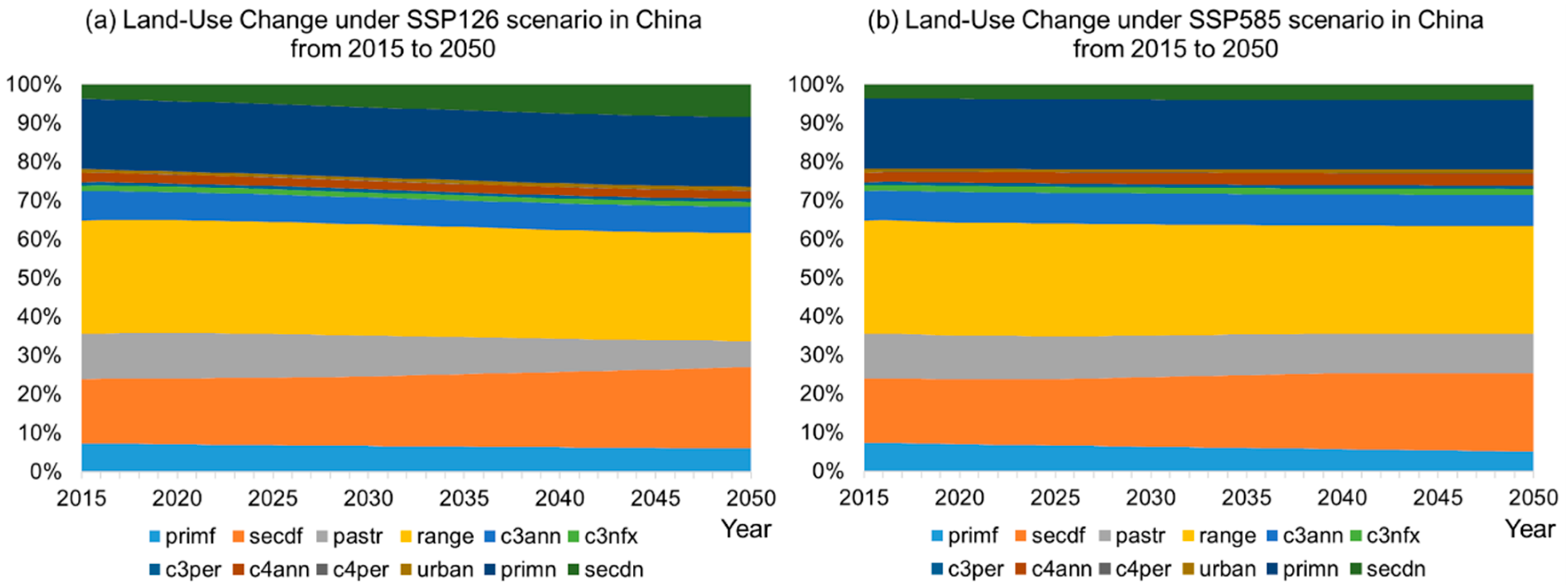
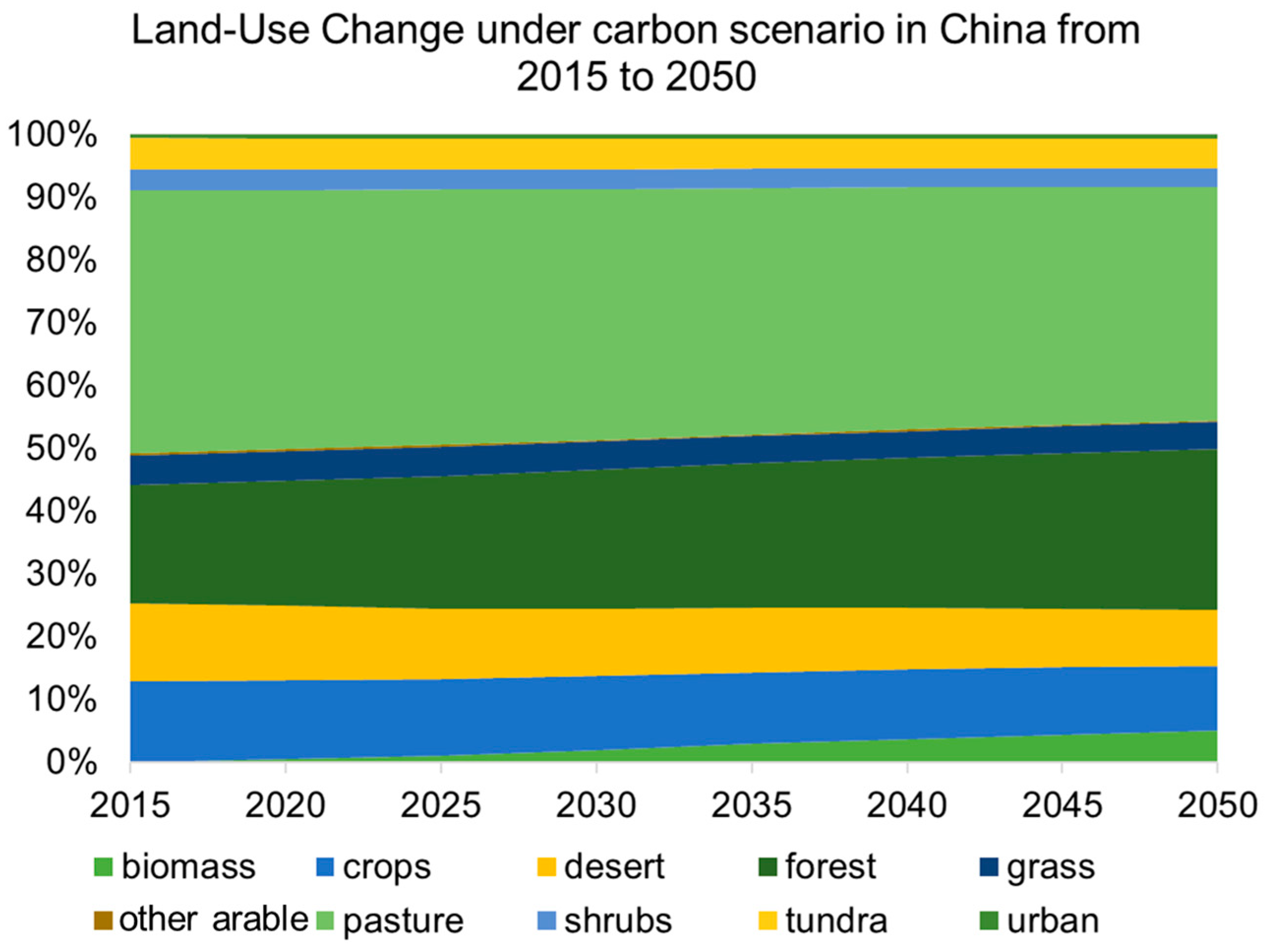
3.1. Land-Use Changes of China from 2015 to 2050 under SSP Scenarios

Figure 2 depicts the evolution of China from 2015 to 2100 under the SSP126 and SSP585 scenarios. In general, the forecast trends of forest land use under the two scenarios were consistent, i.e., primary forest land decreased year after year, while secondary forest land increased year after year, but the SSP126 scenario was more effective in protecting the forest and other vegetation regions. Furthermore, when compared with the SSP585 scenario, the proportion of pastures and range land decreased significantly under the SSP126 scenario.
The differences in the evolution of land-use types under the SSP126 and SSP585 scenarios were determined by the constraints used. With the SSP126 scenario, we aimed to forecast future scenarios based on the green growth paradigm, comprising moderate population growth, economic growth, technological progress, and increased agricultural productivity. Furthermore, this scenario depicted a world concerned with limiting biodiversity loss and reducing the demand for animal products. This scenario considered relevant mitigation policies in order to limit warming to no more than 2 °C. Important policies in terms of global land-use change parameters include increasing the use of bioenergy combined with carbon capture and storage to reduce deforestation and restore degraded forests. In this scenario, the combination of socioeconomic trends and climate policies resulted in a significant reduction in total agricultural land. Simultaneously, large areas were being dedicated to bioenergy production, and the forest area expanded. For example, Figure 3 shows the changes in secdf (secondary forest land) distribution from 2015 to 2050. Increased secdf in southern China may increase BVOC emissions in corresponding regions.
The SSP585 was distinguished by rapid and resource-intensive development that corresponds to material-intensive consumption patterns, as well as technological advances, including agricultural productivity. In the SSP585 scenario, which represented the highest level of emissions, we considered very high levels of fossil fuel use, doubling global food demand, and tripling GHG emissions by 2050. Under the SSP585 scenario, there would be a strong expansion of global cropland into pastures and woodlands, with a global increase of about 300 Mha (20%), a trend that also applied to the downscaling results in China.

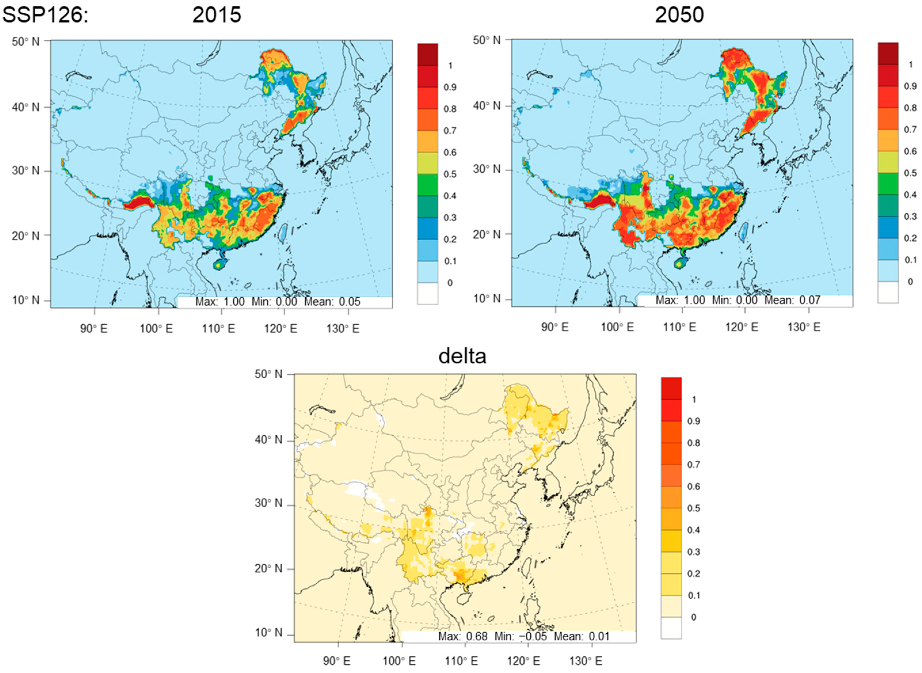
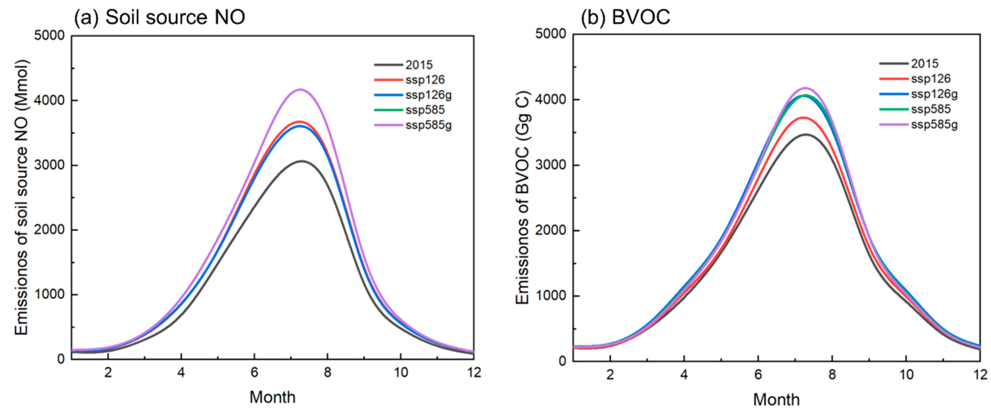
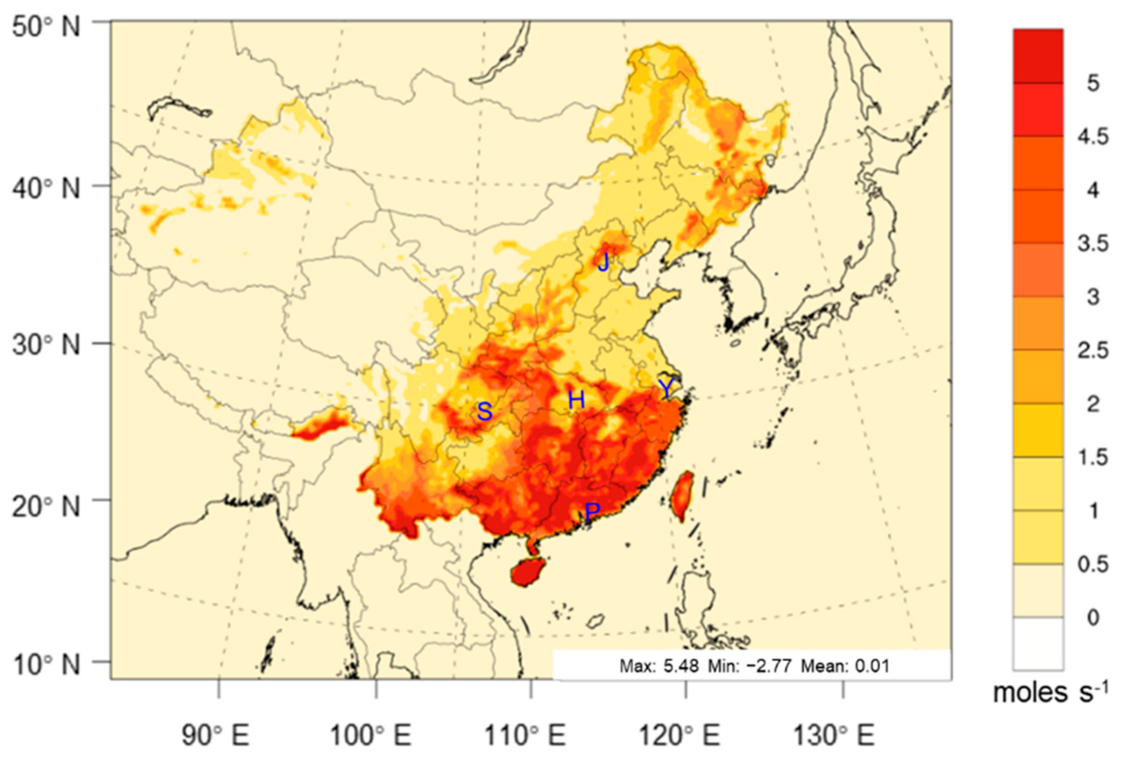
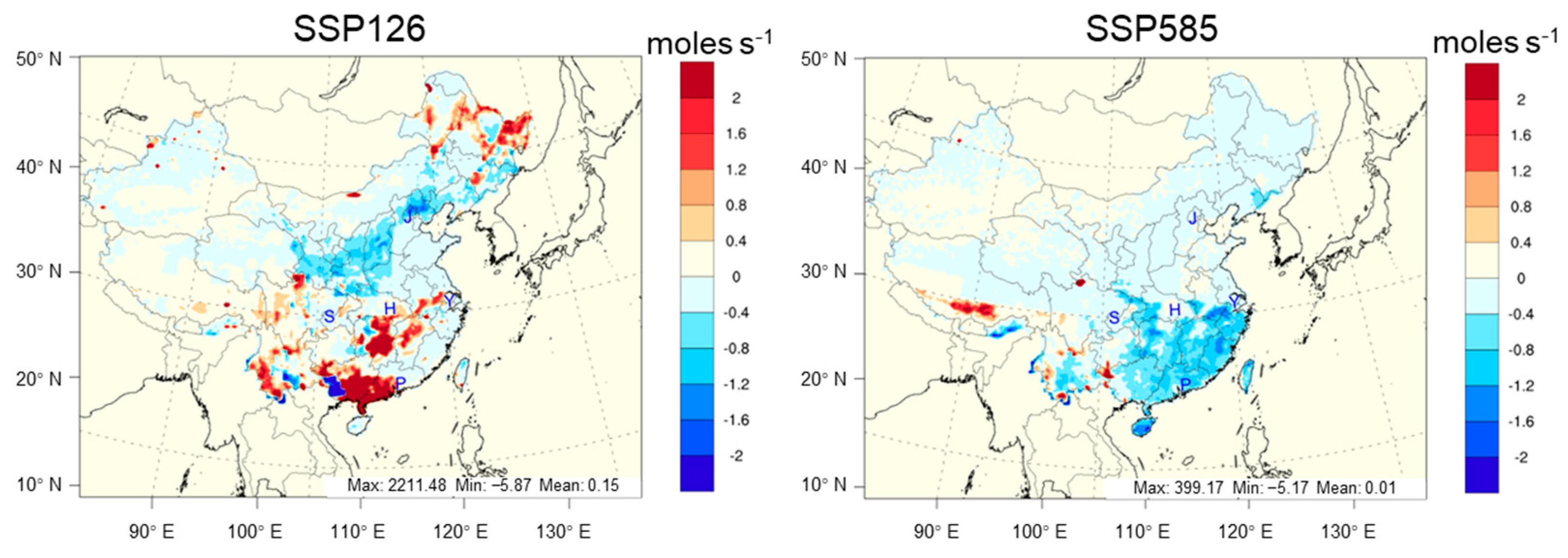
3.2. Changes in BVOC Emissions Driven by Land-Use Changes

Land-use changes directly affect emissions from terrestrial natural sources. Increased vegetation coverage, for example, results in a significant increase in BVOC emissions. We examined the changes in terrestrial natural source emissions driven by land-use change under SSP scenarios from 2015 to 2050. The findings revealed that, after changing land-use type, BVOC emissions changed significantly, whereas changes in soil-source nitric oxide (NO) and dust emissions were still controlled by meteorology. This is because the land-use change data used in this study primarily concern forests, pastures, crops, and other vegetation-related types but do not include the prediction of refined soil types, making BVOC the most sensitive to such changes. Figure 4 depicts the monthly variations in soil-source NO and BVOC emissions in China under various scenarios. The soil-source NO emissions from the five simulation sets showed only three magnitudes that corresponded to their respective input meteorological data, indicating that there were no significant differences between simulations using the same set of meteorological data and different land-use data. BVOC emissions, on the other hand, produced different results. For example, the magnitudes of ssp126 and ssp126g simulation results using the same set of meteorological data but different land data were not the same. In general, the simulated dust emission fluxes of different land-use scenarios under the SSP126 and SSP585 pathways differed by less than 1%, and the annual total soil-source NO emissions were 15.3 Mmol and 17.0 Mmol, respectively, and the changing ratio affected by land-use was 1.3% of the absolute value of emission, which is negligible compared with the proportion of changes caused by meteorological differences. Therefore, we focused on analyzing the response of BVOC in this study.
The monthly BVOC emission variation trend under each scenario was consistent with that of 2015, but the degree of increase from 2015 to 2050 varied. Using the SSP126 pathway as an example, total annual BVOC emissions in 2050 would increase by 6.6%, compared with 2015, reaching 16.9 TgC if the land-use type remains constant. After accounting for land-use change, it would increase by 16.2% (18.5 TgC) in 2050, compared with 2015, equal to the level of BVOC emission increase caused solely by meteorological changes under the SSP585 pathway. Likewise, when the land-use type remained unchanged under the SSP585 pathway, total annual BVOC emissions in 2050 would increase by 15.0%, compared with 2015, reaching 18.3 TgC. After considering the land-use change, it would increase by 15.6% (18.4 TgC) in 2050, compared with 2015, which was comparable to the SSP126 pathway. This is because the increase in forest coverage under the SSP126 land-use change scenario was greater than that under the SSP585 scenario; therefore, the EF corresponding to the BVOC was greater. In comparison, under the SSP585 scenario, temperature and humidity increased more rather than SSP126, leading to more BVOC increase due to meteorological changes than under the SSP126 scenario. However, the BVOC emission of ssp585g in summer was about 1.5% higher than that of ssp126g, due to the more significant climate change in summer under the SSP585 scenario. Overall, the BVOC emissions of each scenario can be divided into four levels based on their temporal variation as in Figure 4b: (1) 2015, (2) SSP126 without land-use changes, (3) SSP126 with land changes and SSP585 without land-use changes, and (4) SSP585 with land-use changes; the last two scenarios were close in magnitude. This study concluded, that under the SSP126 scenario, the impact of land-use changes on BVOC emissions combined with the impact of meteorological changes could equal or even exceed the impact of only meteorological changes under the SSP585 scenario. However, the impact of land-use changes on BVOC emissions under the SSP585 scenario was not obvious. This can be attributed to the impact of meteorological changes, which might have already pushed BVOC emissions to a high level such that the impact of land-use changes was comparatively negligible. In addition, the lower increase in forest land-use type in SSP585, compared with in SSP126 land-use scenario may have also resulted in a lower impact of land-use changes on BVOC emissions in the SSP585 scenario.
Regional differences in the spatial distribution of changes in BVOC emissions were also observed. Figure 5 depicts the impact of land-use changes on BVOC emission rates under the SSP126 and SSP585 pathways, as calculated from ssp126g/ssp585g minus ssp126/ssp585, respectively. Since the land-use changes for each grid were independent, some singularities of abrupt emissions were included, but overall excessive increase and excessive decrease canceled each other out, resulting in average emissions in CHA that were within a reasonable range. Under the SSP126 pathway, land-use changes would reduce BVOC emissions in northern and central China while increasing emissions in southern and northeast China. Such changes are directly related to the evolution of land-use types; for example, the increase in BVOC emissions in the south was linked to the increase in land-use type secdf (secondary forest land) (Figure 3) under the SSP126 scenario. Land-use changes under the SSP585 pathway would reduce BVOC emissions in the south while increasing emissions in the southwest. The BVOC emissions in typical regions were extracted from the impact of land-use changes under two SSP pathways, as listed in Table 3.
Overall, the SSP126 land-use scenario had a greater impact on BVOC emissions (increased by 9.0%) than the SSP585 land-use scenario (increased by 1.8%), which matches the evolution pattern of downscaled LUH2 for the two scenarios indicating a higher increase in forest cover under the SSP126 pathway. The structural adjustment of land-use types was more visible in the SSP126 scenario, such as a significant increase in forest land. Since the vegetation-related land-use type structure in the SSP585 scenario changed less than SSP126, its impact on BVOC emissions was less severe. The downscaling method could capture the characteristics of land-use type changes in different regions under the SSP126 scenario, i.e., forest land increased in southern and northeast China.

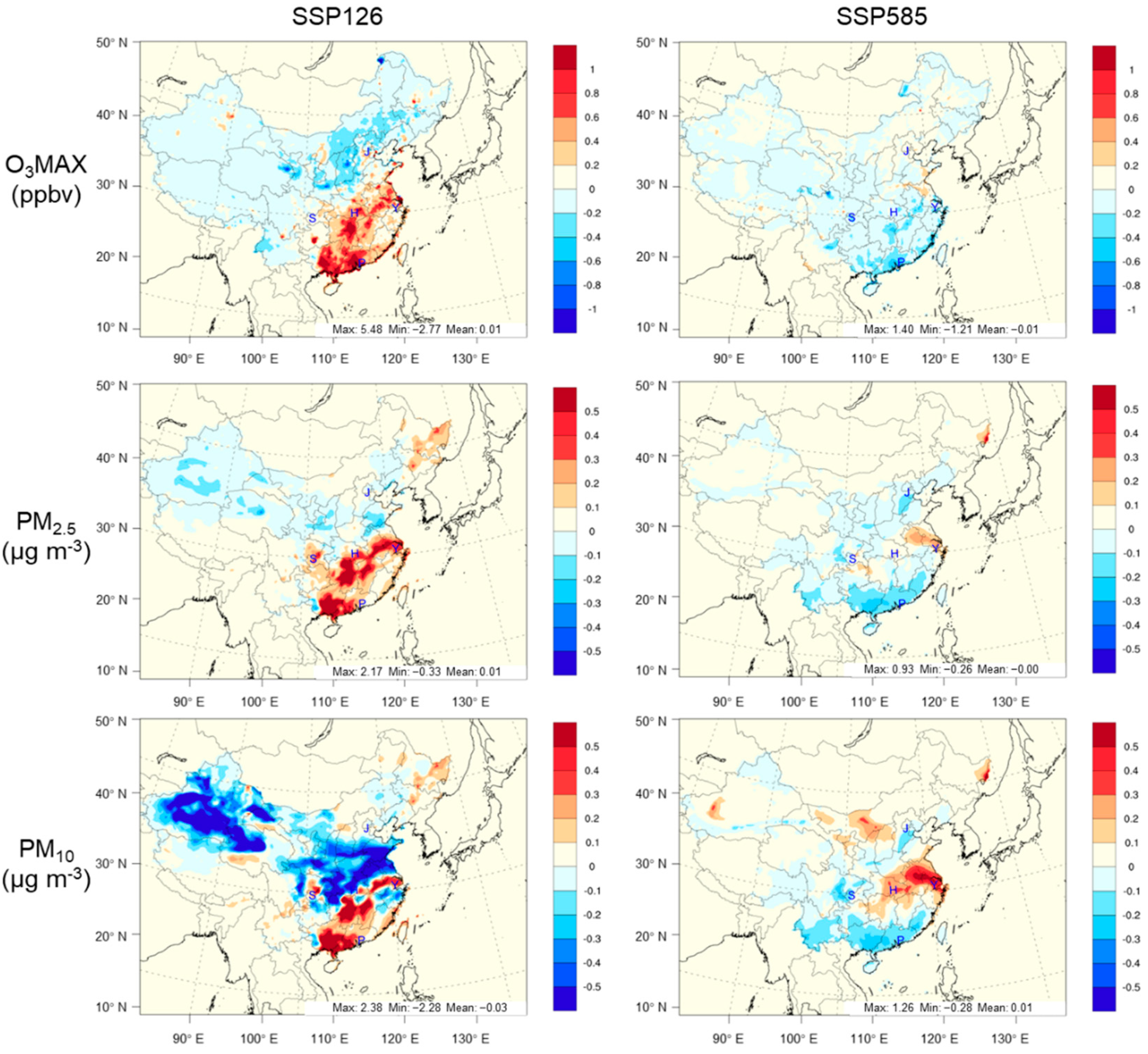
3.3. Changes in O3 and PM Concentrations in Response to Land-Use Changes

Land-use changes further affect the concentration of secondary pollutants by causing terrestrial natural source emissions. Since this study was focused on the impact of land-use change by driving terrestrial natural source emissions, the “effects of land-use change on pollutant concentrations” mentioned in the following text are shorthand for the impact of this mechanism. Under both SSP scenarios, land-use changes decreased O3 concentration by about 0.05 ppbv, increased O3MAX concentration by 0.07 ppbv, and decreased O3MAX concentration by 0.12 ppbv, compared with no land-use change scenarios, on annual average of China, while changes (increased and decreased grids) under SSP126 scenario were more significant. Land-use changes reduced PM2.5 and PM10 concentrations by about 0.05 μg m−3, especially in northwestern China, where PM10 concentrations decreased by 0.24 μg m−3. Figure 6 depicts the annual average concentration changes in O3MAX and PM caused by land-use change under the SSP126 and SSP585 scenarios. The impact of land-use changes was calculated by comparing the simulated concentrations produced using the same meteorological data but different land-use data. The variation trend and degree of O3 and PM concentrations differed due to the varying degree of land-use types in different regions, as listed in Table S2. When compared with the SSP585 scenario, land-use change under the SSP126 scenario had more obvious impacts on O3 and PM, with a decrease in the north and an increase in the south. This suggests that it was easier to control pollutant concentrations under the SSP126 pathway by optimizing land-use types. Furthermore, the effects of land-use changes on O3 and PM concentrations were largely consistent with their effects on BVOC emissions, demonstrating that causing BVOC emissions was the primary mechanism by which land-use changes affected O3 and PM concentrations. Although the overall reduction was still much smaller than the impact of meteorological changes (for example, the impact of meteorological changes on O3, O3MAX, PM2.5, and PM10 under the SSP126 scenario was about 19.6, 2.2, 14.1, and 8.7 times the impact of land-use changes, respectively), it still demonstrates the feasibility of reducing the contribution of terrestrial natural sources by adjusting land-use type structure.
The impact of land-use changes on O3 and PM concentrations was significantly weaker when compared with the impact of meteorological changes. In terms of O3, the annual average change range of each typical area in the two SSP scenarios was roughly 0.4%. In terms of PM, the average annual change in each typical area under the two SSP scenarios was roughly 1.2%. It should be noted that since this study employed relatively high 2015 anthropogenic emissions for 2050 simulations, the impacts of land-use changes may be much higher, considering the significant future anthropogenic emission reductions. Since terrestrial natural source emissions are concentrated in the summer, when land-use type changes, the impact on O3 and PM concentrations are more pronounced in summer due to higher changes in terrestrial natural source emissions. We further extracted the simulation results in typical regions during summer for analysis, as listed in Table S3. Land-use change had a greater impact on the O3 and PM concentrations in summer, and the maximum of summer average change range of the SSP scenario in typical regions expanded to 0.7% and 1.6%, respectively.
The impact of the land-use changes in China on O3 and O3MAX concentrations in summer was approximately twice the annual average level, while the impact on PM2.5 and PM10 was approximately 1.5 times on average of two SSP scenarios. The specific results of each scenario are listed in Table 4.

3.4. Projections under Carbon-Neutral Scenario of China

The land-use change under the carbon scenario was similar to that of SSP126 in terms of vegetation changes. Assuming that forest and cultivated land area conform to national policy, fossil energy would be reduced, biomass ratio would be increased, and the trend of urban development would increase and then decrease. Based on the Global Change Assessment Model (GCAM), we adjusted the land-use type to achieve a peak in carbon emissions in 2030 and carbon neutrality in 2060, as shown in Figure 7. The classification method for land-use types under this scenario differed from that under the SSP scenarios, including biomass (land used for planting energy crops including sugar and oil crops), crops, deserts, forests, grassland, other arable lands, pasture, shrubs, tundra, and urban, which are expressed as biomass, crops, desert, forest, grass, other arable, pasture, shrubs, tundra, and urban in turn, from which the vegetation-related land-use change proportions were extracted to correspond to the SSP scenarios.
Since for the carbon scenario in this study, we used the same meteorological data as those of the SSP126 scenario, the simulated soil-source NO emissions (total 16.1 Mmol) were the same as the results of scenarios using the SSP126 meteorological data but were still 5.3% higher than those of the scenarios that did not consider land-use changes. The annual BVOC emission under the carbon scenario was 24.0 TgC, exceeding the results of all other scenarios, and was 1.4 times higher than that of the SSP126 scenario without considering land-use changes. As a result, land-use changes revealed a higher potential to increase BVOC emissions under the SSP126 pathway, compared with the SSP585 pathway. The monthly variation trends of BVOC and soil-source NO emissions under the carbon scenario were consistent with other scenarios, and the specific emissions are listed in Table S4.
As shown in Figure 8, BVOC emissions in all regions would increase under the carbon scenario when compared with the ssp126 case without accounting for land-use change. Table 5 shows the changes in total BVOC emissions caused by land-use changes in typical regions. Meteorological changes under the SSP126 pathway would increase BVOC emissions in China by 1.0 TgC in 2050, compared with 2015, whereas land-use changes under the carbon scenario would increase them by 7.1 TgC, which is 6.8 times the meteorological impact. On the one hand, under the carbon scenario used in this study, a large number of carbon sinks were added by increasing vegetation coverage in order to achieve the goals of “carbon peaking” and “carbon neutrality”, and the vegetation growth estimation was relatively aggressive. On the other hand, if vegetation coverage is greatly increased in the future, BVOC emissions will continue to rise and cannot be ignored.
Under the carbon scenario, land-use changes increased O3 and O3MAX concentrations by 0.06 ppbv and 0.70 ppbv, respectively, with an average annual change of less than 1.6%, much less than the impact of meteorological changes. The land-use changes resulted in increased PM2.5 and PM10 concentrations by 0.16 μg m−3 and 0.28 μg m−3, respectively, with an average annual change range of less than 3.6%. Figure 9 depicts the impact of land-use change on pollutant concentrations under the carbon scenario, and Table 6 lists specific results in typical regions. Under the carbon scenario, land-use change showed the potential to increase pollutant concentrations. The land-use change had a greater impact on O3 and PM concentrations during the summer, with maximum ratios of about 3.2% and 6.2%, respectively. The ratios of the impact of land-use changes on the concentration of O3, O3MAX, PM2.5, and PM10 concentrations in summer and the annual average level were 3.77, 2.68, 2.16, and 1.61, respectively. The PM2.5 concentration in PRD and HUZ was significantly increased by more than 0.5 μg m−3 in summer. To ensure air quality (the WHO annual PM2.5 limit of 5 μg m−3), potential risks must be mitigated or offset through anthropogenic emission control.

4. Summary

This study predicted three future land-use type scenarios in 2050 (SSP126, SSP585, and carbon scenario) based on downscaled LUH2 data and carbon-neutral policy in China. We quantified the contribution of land-use changes to terrestrial natural source BVOC emissions, as well as O3 and PM concentrations.
Land-use changes directly affect emissions from terrestrial natural sources. The variation ranges of wind-blown dust and soil-source NO emissions were less than 1.3%, far less than the impact of meteorological changes. BVOC emission changes are sensitive to land-use type. After adjusting the land-use type, the rate of increase in BVOC emissions under the SSP126 pathway could reach the level caused only by meteorological changes under the SSP585 pathway. Under the SSP126 pathway, meteorological changes would increase BVOC emissions in China by 1.0 TgC in 2050 compared with 2015, while land-use changes would increase them by 1.5–7.1 TgC, up to 6.8 times the meteorological impact. If vegetation coverage is significantly increased in the future, the resulting increase in BVOC emissions cannot be ignored. The SSP126 land-use scenario had a greater impact on BVOC emissions than the SSP585 land-use scenario, which was consistent with the evolution characteristics obtained after downscaling the two LUH2 scenarios.
The impact of land-use changes on O3 and PM concentrations (by causing terrestrial natural source emissions) was essentially the same trend as their impact on BVOC emissions, which was greater in summer (about twice the annual average level), demonstrating that the driving force behind BVOC emissions is the impact mechanism of land-use changes on O3 and PM concentrations. The land-use change caused a significant decrease in PM10 concentration in northwestern China under the SSP126 scenario, demonstrating the feasibility of reducing the contribution of terrestrial natural sources by adjusting the structure of land-use types. Overall, land-use changes had a weaker impact on O3 and PM concentrations than meteorological changes. The average annual change in each scenario was within a 3.6% limit and larger in summer (within 6.2%). Regional differences must be considered when calculating future pollutant background concentrations in the environment. The impact of land-use change on pollutants was more obvious under the SSP126 pathway than under the SSP585 pathway, indicating that more attention should be paid to optimizing land-use types under the SSP126 pathway. Under the carbon scenario, the increase in PM concentration caused by terrestrial natural sources as a result of land-use change would pose a risk to air quality compliance; thus, it is necessary to consider reducing or offsetting this potential risk through anthropogenic emission control measures.

Supplementary Materials

The following supporting information can be downloaded at: www.mdpi.com/article/10.3390/atmos13071086/s1, Table S1: Fitting results of the relationship between FPAR and LAI; Table S2: Impact of land−use changes on annual average O3 (unit: ppbv) and PM (unit: μg m−3) concentra-tions in typical regions under SSP scenarios; Table S3: Impact of land−use changes on O3 (unit: ppbv) and PM (unit: μg m−3) concentrations in typical regions in summer under SSP scenarios; Table S4. Monthly average BVOC and soil-source NO emissions under carbon scenario.

Author Contributions

Data curation, S.L. (Song Liu), S.K.S., S.L. (Shuchang Liu), Y.S. and H.Z.; formal analysis, S.L. (Song Liu); funding acquisition, J.X. and S.W.; methodology, S.L. (Song Liu), S.K.S., J.X. and B.Z.; supervision, J.X. and S.W.; writing—original draft preparation, S.L. (Song Liu); writing—review and editing, S.K.S., S.Z., X.L. and J.X. All authors have read and agreed to the published version of the manuscript.

Funding

This study was supported in part by the National Natural Science Foundation of China (4190070530 & 51861135102).

Institutional Review Board Statement

Not applicable.

Informed Consent Statement

Not applicable.

Acknowledgments

This study was completed on the “Explorer 100” cluster system of Tsinghua National Laboratory for Information Science and Technology.

Conflicts of Interest

The authors declare no conflict of interest.

References

  1. Cohen, A.J.; Brauer, M.; Burnett, R.; Anderson, H.R.; Frostad, J.; Estep, K.; Balakrishnan, K.; Brunekreef, B.; Dandona, L.; Dandona, R. Estimates and 25-year trends of the global burden of disease attributable to ambient air pollution: An analysis of data from the Global Burden of Diseases Study 2015. Lancet 2017, 389, 1907–1918. [Google Scholar] [CrossRef] [Green Version]
  2. Lin, Y.; Jiang, F.; Zhao, J.; Zhu, G.; He, X.; Ma, X.; Li, S.; Sabel, C.E.; Wang, H. Impacts of O3 on premature mortality and crop yield loss across China. Atmos. Environ. 2018, 194, 41–47. [Google Scholar] [CrossRef]
  3. Ding, D.; Xing, J.; Wang, S.; Liu, K.; Hao, J. Estimated contributions of emissions controls, meteorological factors, population growth, and changes in baseline mortality to reductions in ambient PM2.5 and PM2.5-related mortality in China, 2013–2017. Environ. Health Perspect. 2019, 127, 067009. [Google Scholar] [CrossRef]
  4. Liu, S.; Xing, J.; Zhang, H.; Ding, D.; Zhang, F.; Zhao, B.; Sahu, S.K.; Wang, S. Climate-driven trends of biogenic volatile organic compound emissions and their impacts on summertime ozone and secondary organic aerosol in China in the 2050s. Atmos. Environ. 2019, 218, 117020. [Google Scholar] [CrossRef]
  5. Thunis, P.; Cuvelier, C. Impact of biogenic emissions on ozone formation in the Mediterranean area—A BEMA modelling study. Atmos. Environ. 2000, 34, 467–481. [Google Scholar] [CrossRef]
  6. Ma, M.; Gao, Y.; Wang, Y.; Zhang, S.; Leung, L.R.; Liu, C.; Wang, S.; Zhao, B.; Chang, X.; Su, H.; et al. Substantial ozone enhancement over the North China Plain from increased biogenic emissions due to heat waves and land cover in summer 2017. Atmos. Chem. Phys. Discuss. 2019, 2019, 12195–12207. [Google Scholar] [CrossRef] [Green Version]
  7. Zhang, Y.; Wang, Y. Climate-driven ground-level ozone extreme in the fall over the Southeast United States. Proc. Natl. Acad. Sci. USA 2016, 113, 10025–10030. [Google Scholar] [CrossRef] [Green Version]
  8. Carlton, A.; Wiedinmyer, C.; Kroll, J. A review of Secondary Organic Aerosol (SOA) formation from isoprene. Atmos. Chem. Phys. Discuss. 2009, 9, 4987–5005. [Google Scholar] [CrossRef] [Green Version]
  9. Zhang, Y.; Hu, X.M.; Leung, L.R.; Gustafson, W.I. Impacts of regional climate change on biogenic emissions and air quality. J. Geophys. Res. Atmos. 2008, 113, D18310. [Google Scholar] [CrossRef] [Green Version]
  10. Jang, Y.; Eo, Y.; Jang, M.; Woo, J.H.; Lim, J.H. Impact of Land Cover and Leaf Area Index on BVOC Emissions over the Korean Peninsula. Atmosphere 2020, 11, 806. [Google Scholar] [CrossRef]
  11. Wang, H.; Wu, Q.; Guenther, A.B.; Yang, X.; Cheng, H. A long-term estimation of biogenic volatile organic compound (BVOC) emission in China from 2001–2016: The roles of land cover change and climate variability. Atmos. Chem. Phys. 2021, 21, 4825–4848. [Google Scholar] [CrossRef]
  12. Dong, X.; Fu, J.S.; Huang, K.; Tong, D.; Zhuang, G. Model development of dust emission and heterogeneous chemistry within the Community Multiscale Air Quality modeling system and its application over East Asia. Atmos. Chem. Phys. 2016, 16, 8157–8180. [Google Scholar] [CrossRef] [Green Version]
  13. Liu, S.; Xing, J.; Sahu, S.K.; Liu, X.; Liu, S.; Jiang, Y.; Zhang, H.; Li, S.; Ding, D.; Chang, X. Wind-blown dust and its impacts on particulate matter pollution in Northern China: Current and future scenarios. Environ. Res. Lett. 2021, 16, 114041. [Google Scholar] [CrossRef]
  14. Jiang, X.; Wiedinmyer, C.; Chen, F.; Yang, Z.-L.; Chun-Fung, J. Predicted impacts of climate and land use change on surface ozone in the Houston, Texas, area. J. Geophys. Res. Atmos. 2008, 113, D20. [Google Scholar] [CrossRef]
  15. Feng, C.; Li, R. Spatiotemporal variation analysis of air pollution from 2013 to 2019 in Beijing based on land use regression model. Huanjing Kexue Xuebao Acta Sci. Circumstantiae 2021, 41, 1231–1238. [Google Scholar] [CrossRef]
  16. Liu, Y.; Paciorek, C.J.; Koutrakis, P. Estimating Regional Spatial and Temporal Variability of PM2.5 Concentrations Using Satellite Data, Meteorology, and Land Use Information. Environ. Health Perspect. 2009, 117, 886–892. [Google Scholar] [CrossRef] [Green Version]
  17. Hurtt, G.C.; Chini, L.P.; Frolking, S.; Betts, R.A.; Feddema, J.; Fischer, G.; Fisk, J.P.; Hibbard, K.; Houghton, R.A.; Janetos, A.; et al. Harmonization of land-use scenarios for the period 1500–2100: 600 years of global gridded annual land-use transitions, wood harvest, and resulting secondary lands. Clim. Chang. 2011, 109, 117. [Google Scholar] [CrossRef] [Green Version]
  18. Prestele, R.; Alexander, P.; Rounsevell, M.D.; Arneth, A.; Calvin, K.; Doelman, J.; Eitelberg, D.A.; Engström, K.; Fujimori, S.; Hasegawa, T. Hotspots of uncertainty in land-use and land-cover change projections: A global-scale model comparison. Glob. Chang. Biol. 2016, 22, 3967–3983. [Google Scholar] [CrossRef] [Green Version]
  19. Verburg, P.H.; Tabeau, A.; Hatna, E. Assessing spatial uncertainties of land allocation using a scenario approach and sensitivity analysis: A study for land use in Europe. J. Environ. Manag. 2013, 127, S132–S144. [Google Scholar] [CrossRef]
  20. Liao, W.; Liu, X.; Xu, X.; Chen, G.; Li, X. Projections of land use changes under the plant functional type classification in different SSP-RCP scenarios in China. Sci. Bull. 2020, 65, 1935–1947. [Google Scholar] [CrossRef]
  21. Xinhua. Xi Jinping Delivers an Important Speech at the General Debate of the 75th General Assembly of the United Nations. Available online: http://www.xinhuanet.com/politics/leaders/2020-09/22/c_1126527647.htm (accessed on 20 May 2022).
  22. Byun, D.W.; Pleim, J.E.; Tang, R.T.; Bourgeois, A. Meteorology-Chemistry Interface Processor (MCIP) for Models-3 Community Multiscale Air Quality (CMAQ) Modeling System; US Environmental Protection Agency, Office of Research and Development: Washington, DC, USA, 1999. [Google Scholar]
  23. Guenther, A.B.; Jiang, X.; Heald, C.L.; Sakulyanontvittaya, T.; Duhl, T.; Emmons, L.K.; Wang, X. The Model of Emissions of Gases and Aerosols from Nature version 2.1 (MEGAN2.1): An extended and updated framework for modeling biogenic emissions. Geosci. Model Dev. 2012, 5, 1471–1492. [Google Scholar] [CrossRef] [Green Version]
  24. Byun, D.W.; Ching, J. Science Algorithms of the EPA Models-3 Community Multiscale Air Quality (CMAQ) MODELING System; US Environmental Protection Agency, Office of Research and Development: Washington, DC, USA, 1999. [Google Scholar]
  25. Jiang, X.; Guenther, A.; Potosnak, M.; Geron, C.; Seco, R.; Karl, T.; Kim, S.; Gu, L.; Pallardy, S. Isoprene Emission Response to Drought and the Impact on Global Atmospheric Chemistry. Atmos. Environ. 2018, 183, 69–83. [Google Scholar] [CrossRef]
  26. Zhang, M.; Zhao, C.; Yang, Y.; Du, Q.; Shen, Y.; Lin, S.; Gu, D.; Su, W.; Liu, C. Modeling sensitivities of BVOCs to different versions of MEGAN emission schemes in WRF-Chem (v3.6) and its impacts over eastern China. Geosci. Model Dev. 2021, 14, 6155–6175. [Google Scholar] [CrossRef]
  27. Liu, S.; Xing, J.; Wang, S.; Ding, D.; Hao, J. Health Benefits of Emission Reduction under 1.5 °C Pathways Far Outweigh Climate-Related Variations in China. Environ. Sci. Technol. 2021, 55, 10957–10966. [Google Scholar] [CrossRef]
  28. Hu, J.; Wang, P.; Ying, Q.; Zhang, H.; Chen, J.; Ge, X.; Li, X.; Jiang, J.; Wang, S.; Zhang, J. Modeling biogenic and anthropogenic secondary organic aerosol in China. Atmos. Chem. Phys. 2017, 17, 77–92. [Google Scholar] [CrossRef] [Green Version]
  29. Zheng, H.; Zhao, B.; Wang, S.; Wang, T.; Ding, D.; Chang, X.; Liu, K.; Xing, J.; Dong, Z.; Aunan, K. Transition in source contributions of PM2.5 exposure and associated premature mortality in China during 2005–2015. Environ. Int. 2019, 132, 105111. [Google Scholar] [CrossRef]
  30. Zhao, B.; Zheng, H.; Wang, S.; Smith, K.R.; Lu, X.; Aunan, K.; Gu, Y.; Wang, Y.; Ding, D.; Xing, J. Change in household fuels dominates the decrease in PM2.5 exposure and premature mortality in China in 2005–2015. Proc. Natl. Acad. Sci. USA 2018, 115, 12401–12406. [Google Scholar] [CrossRef] [Green Version]
  31. Stohl, A.; Aamaas, B.; Amann, M.; Baker, L.; Bellouin, N.; Berntsen, T.K.; Boucher, O.; Cherian, R.; Collins, W.; Daskalakis, N. Evaluating the climate and air quality impacts of short-lived pollutants. Atmos. Chem. Phys. 2015, 15, 10529–10566. [Google Scholar] [CrossRef] [Green Version]
  32. Gower, S.T.; Kucharik, C.J.; Norman, J.M. Direct and Indirect Estimation of Leaf Area Index, fAPAR, and Net Primary Production of Terrestrial Ecosystems. Remote Sens. Environ. 1999, 70, 29–51. [Google Scholar] [CrossRef]
  33. Zhao, B.; Wang, S.; Wang, J.; Fu, J.S.; Liu, T.; Xu, J.; Fu, X.; Hao, J. Impact of national NOx and SO2 control policies on particulate matter pollution in China. Atmos. Environ. 2013, 77, 453–463. [Google Scholar] [CrossRef]
  34. Streets, D.G.; Fu, J.S.; Jang, C.J.; Hao, J.; He, K.; Tang, X.; Zhang, Y.; Wang, Z.; Li, Z.; Zhang, Q.; et al. Air quality during the 2008 Beijing Olympic Games. Atmos. Environ. 2007, 41, 480–492. [Google Scholar] [CrossRef]
  35. Wang, L.; Xu, J.; Yang, J.; Zhao, X.; Wei, W.; Cheng, D.; Pan, X.; Su, J. Understanding haze pollution over the southern Hebei area of China using the CMAQ model. Atmos. Environ. 2012, 56, 69–79. [Google Scholar] [CrossRef]
  36. Liu, S.; Xing, J.; Westervelt, D.M.; Liu, S.; Ding, D.; Fiore, A.M.; Kinney, P.L.; Zhang, Y.; He, M.Z.; Zhang, H. Role of emission controls in reducing the 2050 climate change penalty for PM2. 5 in China. Sci. Total Environ. 2020, 765, 144338. [Google Scholar] [CrossRef]
  37. Emery, C.; Tai, E.; Yarwood, G. Enhanced Meteorological Modeling and Performance Evaluation for Two Texas Ozone Episodes; Environ, International Corporation: Novato, CA, USA, 2001. [Google Scholar]
Figure 1. The modeling domain with a grid resolution of 27 km (182 × 232 cells) and the locations of the five typical regions (i.e., JJJ, YRD, PRD, SCH, and HUZ. J, Y, P, S, and H are marked in the center of the regions in the following figures), eastern China (ECH), and mainland China (CHA, shaded part).
Atmosphere 13 01086 g001
Figure 2. Evolution of land-use types in China from 2015 to 2100 under (a) SSP126 and (b) SSP585 scenarios (primary forest, secondary forest land, managed pastures, other pastures, C3 annual crops, C3 nitrogen-fixing crops, C3 perennial crops, C4 annual crops, C4 perennial crops, urban, primary non-forest land, and secondary non-forest vegetation land, denoted as primf, secdf, pastr, range, c3ann, c3nfx, c3per, c4ann, c4per, urban, primn, and secdn, respectively).
Atmosphere 13 01086 g002
Figure 3. Changes in proportion of land-use type secdf between in 2015 and in 2050.
Atmosphere 13 01086 g003
Figure 4. Monthly variations in (a) soil-source NO and (b) BVOC emissions under various SSP scenarios.
Atmosphere 13 01086 g004
Figure 5. Impact of land-use change on the rate of BVOC emissions under the SSP scenario (unit: moles s−1).
Atmosphere 13 01086 g005
Figure 6. Impact of land-use change on O3MAX, PM2.5, and PM10 concentrations under SSP scenarios.
Atmosphere 13 01086 g006
Figure 7. Land-use change in China from 2015 to 2050 under carbon scenario.
Atmosphere 13 01086 g007
Figure 8. Impact of land-use changes on BVOC emission rates under the carbon scenario (Unit: moles s−1).
Atmosphere 13 01086 g008
Figure 9. Impact of land-use change on pollutant concentrations under the carbon scenario.
Atmosphere 13 01086 g009
Table 1. Fitting coefficients for each variable in the carbon scenario using the ratio method.
VariableCoefficient
LAI1.291
EFISOP (isoprene)1.408
MYRC (myrcene)1.493
SABI (sabinene)1.486
LIMO (limonene)1.490
A_3CAR (3-carene)1.494
OCIM (t-β-ocimene)1.477
BPIN (β-pinene)1.488
APIN (α-pinene)1.494
MBO (232-MBO)1.500
Table 2. Simulation cases in this study.
GroupMeteorological DataLand-Use DataCase Name
base20152015base
SSP126SSP1262015ssp126
SSP126SSP126 gridssp126g
SSP585SSP5852015ssp585
SSP585SSP585 gridssp585g
carbonSSP126Carbon ratiocarbon
Table 3. Impact of land-use change on BVOC emissions in typical regions under the SSP scenarios (unit: GgC).
RegionSSP126SSP585
JJJ−71.4−0.1
YRD4.0−24.3
PRD32.9−26.4
SCH2.8−37.1
HUZ36.3−27.2
ECH321.476.2
CHA2389.784.3
Table 4. The ratio of impact of land-use changes on the concentration of O3 and PM concentrations in summer to the annual average level.
RegionVariableSSP126SSP585
CHAO3 (ppbv)2.932.92
O3MAX (ppbv)1.421.43
PM2.5 (μg m−3)2.181.14
PM10 (μg m−3)2.221.11
Table 5. Impact of land-use changes on BVOC emissions in typical regions under the carbon scenario.
RegionJJJYRDPRDSCHHUZECHCHA
Changes
(Unit: GgC)
239.9122.4178.7417.3269.74857.47061.0
Table 6. Impact of land-use change on O3 (unit: ppbv) and PM (unit: μg m−3) concentrations in typical regions under carbon scenario.
VariablesJJJYRDPRDSCHHUZECHCHA
AnnualO30.420.350.340.320.530.220.06
O3MAX0.700.690.600.680.320.790.70
PM2.50.220.270.530.270.610.260.16
PM100.380.440.770.570.920.430.28
SummerO31.090.820.660.731.060.540.24
O3MAX1.811.811.261.640.621.881.88
PM2.50.700.720.670.831.260.560.35
PM100.870.930.891.211.580.740.45
Publisher’s Note: MDPI stays neutral with regard to jurisdictional claims in published maps and institutional affiliations.

