Abstract
Air pollution is a global problem that is responsible for more than four million premature deaths each year. Air exchange in ammonia engine rooms is a priority for normal operating conditions, as well as in the event of an emergency release. A numerical approach with the use of computational fluid dynamics techniques can provide detailed data, such as spatial gas dispersion. Therefore, the objective of this study was to prepare a mathematical tool for the assessment of ammonia distribution in an engine room equipped with forced ventilation as a prediction tool for dangerous industrial setup working configurations. This study analyzed the uncontrolled release of ammonia during the production process in an engine room using Ansys Fluent software. It was observed that emergency ammonia leakage of 0.1 kg/s in the assumed air flow poses a great threat to the mechanics. In many simulated scenarios, ammonia spread to the entire building. Moreover, the mass fraction of ammonia was the highest in the gas stream right after its release. After being released, ammonia often accumulated in the ceiling zone, and in inactive exhaust chimneys, air inlets, and doors. It was observed that the effectiveness of the ventilation analyzed depended on the number of active air vents and exhausts, as well as their spatial distribution throughout the building.
1. Introduction
A hazardous chemical leakage accident may occur in the process of production, transportation, and storage []. Ammonia is used in several segments of the chemical industry, for example, in the pharmaceutical, textile, and industrial refrigeration industries []. It is one of the predominant gaseous pollutants []. According to the World Health Organization (WHO), air pollution is the main contributor to the increasing number of diseases, e.g., respiratory infections []. In the last few decades, attempts have been made in the field of indoor environments to find a balance between air distribution, indoor air quality, and energy efficiency []. Air exchange in ammonia engine rooms is a priority both during normal operating conditions and in the event of an emergency release, e.g., due to valve leakage. The main problem of these constructions is related to insufficient ventilation systems []. The appropriate capacity of exhaust fans, as well as ventilation openings, provides air circulation in a building with an ammonia system to operate smoothly []. Moreover, people spend more than 90% of their time indoors, and the level of indoor air pollution is generally higher than that of the outdoor environment []. Thus, indoor air quality is essential for human health, productivity, and well-being []
The description of ammonia dispersion focuses mainly on toxic gas leakage. Due to personnel operation faults, equipment failure, and poor safety management, toxic gas leakage accidents may occur in chemical plants []. To support decisions in the case of the dispersion of hazardous gases, mathematical tools are applied [,]. Mathematical operations may be performed analytically, with physical equations or by implementing those equations into appropriate software []. Furthermore, dispersion models can be described as Gaussian, integral-type, and computational fluid dynamics (CFD) models []. Among all models presented, ALOHA, PHAST, and CFD codes are the most commonly used to study gas dispersion [,]. Furthermore, CFD is a useful tool for estimating hazardous zones after the release of flammable gases []. This approach uses Navier–Stokes equations for simulation with CFD tools, consisting of a set of nonlinear momentum and mass conservation equations to estimate the pressure distributions in each zone and to calculate the airflow through the zones []. The group of CFD models includes three subgroups of the following models: RANS (Reynolds-averaged Navier–Stokes equations), LES (large-eddy simulations) and DNS (direct numerical simulations) []. Moreover, many previous CFD studies have indicated that the appropriate choice of Reynolds-averaged Navier–Stokes (RANS) turbulence model is important in reproducing heavy gas dispersion. Sklavounos and Rigas found that the standard keε and shear stress transport (SST) k-u models appeared to overestimate the maximal concentrations recorded in the trials []. Conversely, Xing et al. showed that the results from the standard k-ε and SST k-u models were in acceptable agreement with the experimental data, while the predicted values from the RNG k-ε model were unsatisfactory []. Moreover, many previous CFD studies have indicated that the appropriate choice of RANS turbulence models is important in reproducing heavy gas dispersion; however, there is not a consistent conclusion regarding which model is better for simulating heavy gas dispersion [].
Due to the flammable and toxic properties of ammonia, the risk caused by the release of ammonia to the atmosphere due to tank failure, road collision, or the ammonia engine room is high. Therefore, the objective of this study was to prepare a mathematical tool for the assessment of the ammonia distribution in an engine room equipped with forced ventilation as an engineering tool for the prediction of dangerous working conditions of industrial setups.
The paper is organized as follows: In Section 2, a description of the analyzed case study, as well as material and methods applied in the research, are presented. Section 3 presents the results of the numerical simulations. In Section 4, a discussion is presented, while Section 5 concludes the manuscript.
2. Materials and Methods
2.1. Case Study
This study analyzed uncontrolled ammonia release in the production process in an engine room (length—9 m, width—5 m, height—4 m) in an industrial plant (Figure 1). Each front wall of the building was equipped with a door (height—2 m, width—1 m) and two ventilation openings (0.75 m × 0.25 m) for each. In addition, there are three cylindrical chimneys (exhausts) with an internal diameter of 0.7 m and a length of 1.2 m in the roof of the mathematical domain analyzed. In the center of the building there is a cylindrical tank (diameter—1 m, length—3 m) containing ammonia gas. Around the tank, a system of pipes was modeled that transports ammonia gas to other facilities of the plant. Furthermore, there are two outlets (diameter—0.3 m), simulating an emergency release of ammonia in the center of the pipe surrounding the ammonia tank.
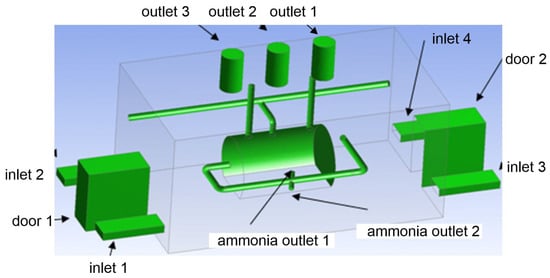
Figure 1.
Three-dimensional geometry of the analyzed ammonia machine room.
2.2. Mathematical Description
First, the 3d model of the mathematical domain analyzed was prepared with the use of SpaceClaim Ansys software (ANSYS, Canonsburg, PA, USA) (Figure 1). In the next step, with the use of Ansys ICEM software (ANSYS, Canonsburg, PA, USA), a numerical mesh was designed []. To reduce discretization errors, a mesh independent test was performed. Thus, different sizes of mesh elements were tested. The range of elements tested for the whole analyzed domain was equal to 0.05–0.1 m (with size increase equal to 0.01 m), decreasing the size of the elements to 0.05 m around the wall. Each time, for the element size equal to 0.1, errors appeared. However, for the grid composed of smaller elements (0.05 m), the CFD model presented converged results (Table 1). Thus, to minimize the size of the numerical mesh, the final mesh consisted of 750,000 tetrahedral elements, and was composed of elements with sizes equal to 0.05 m for the areas where the greatest gradients of the analyzed parameters were expected.

Table 1.
Results for the mesh independent test.
Numerical analysis was performed with the use of Reynolds-averaged Navier–Stokes equations implemented in Ansys Fluent software (ANSYS, Canonsburg, PA, USA) [].
Reynolds-averaged Navier–Stokes equations (Equations (1) and (2)) were applied [,]:
where ρ is the density; t is time; ui and uj are the mean velocity components in the xi and xj directions, respectively; and μ is dynamic viscosity. Moreover, the relationship between the Reynolds stresses and the mean velocity gradients is shown in Equation (3).
where μt is turbulent viscosity; k is turbulent kinetic energy; and δij is the Kronecker delta. K and its rate of dissipation ε are obtained from Equations (4) and (5).
Furthermore, in this work, the k–ε model was used to represent the effects of turbulence [].
where Gk is the generation of k due to the mean velocity gradient, and σk and σε are the turbulent Prandtl numbers for k and ε, respectively.
The turbulent (or eddy) viscosity μt is computed by combining k and ε (Equation (6)).
Furthermore, results were presented as isosurfaces and isolines. For the Ansys Fluent software, the Reynolds-averaged Navier–Stokes (RANS) model was applied.
The following boundary conditions were established: (1) the initial pressure was equal to 1013 hPa for each outlet; (2) the air exchange in the building took place through three exhaust fans located on the ceiling of the building with a diameter equal to 0.7 m and a length equal to 1.2 m each; (3) the emergency flow of ammonia occurred from two nozzles, one directed with the cross-sectional plane upwards, and the other downwards. Furthermore, at least one surface from inlet 1, inlet 2, inlet 3, and inlet 4 was the inlet with a defined initial velocity in the range of 1 m/s to 3 m/s. The outlet of the tested model was determined from among outlet 1, outlet 2, and outlet 3. One of these surfaces was a pressure outlet with a pressure value equal to 0 Pa. Then, the ammonia 1 outlet and the ammonia 2 outlet were set as mass flow and equal to 0.1 kg/s. Other surfaces, such as the outline of the ammonia engine room, the door, the ammonia tank, and the pipes exiting the tank, were established as the wall boundary. Moreover, the air temperature was equal to 25 °C. Table 2 presents all analyzed cases.
Table 2.
Analyzed cases of ammonia release and work of the ventilation system. V—variant; S—scenario.
3. Results
The distribution of ammonia concentration is the most significant concern due to toxicity. Ammonia is widely used in the chemical and food industry as a common industrial gas []. According to the National Fire Protection Association guidelines, the ammonia–air mixture is combustible in the concentration range of 15–28% [].
The first variant analyzed contained four scenarios (from A to D) with ammonia discharge rate equal to 0.1 kg/s and only one active exhaust chimney (outlet 3) (Figure 2 and Figure 3). The outflow of ammonia was set at the upper outlet connection. In scenario A, it was assumed that the air inflow to the engine room would occur through the inlet no. 2. In this case, the air velocity at the inlet was equal to 2.2 m/s, and at the outlet it was in the range of 1.4 to 1.5 m/s. Moreover, it was noticed that the cloud occupied a small area and volume of the analyzed domain. Furthermore, after it was released, the ammonia was directed towards the exhaust stack. Scenario B assumed the airflow into the building through inlet no. 4. The velocity of the air was the same as in scenario A. It was noticed that the air flowed low through the engine room and that turbulence occurred at the height of the active exhaust chimney. As a result, ammonia spread throughout the building, and the largest mass fraction equal to approximately 0.7 was observed in the inactive chimney no. 1 and in the ceiling zone within this chimney. In scenario C, it was assumed that the air stream flowed into the room through inlet no. 1 and inlet no. 2. In this case, the air velocity was equal to 1 m/s in each of the inlets and 1.4 m/s in the exhaust chimney. Trace amounts of ammonia were observed in chimney no. 1, in door no. 2, inlet no. 3, and between the ammonia tank and inlet no. 3. In addition, the largest ammonia mass fraction was found in a small cloud near the tank. In scenario D, the active air inlets in the engine room were inlet no. 2 and inlet no. 4. The air velocity was equal to the velocity in scenario C. In this scenario, it was observed that air flowed in opposite directions and caused a turbulence appearance, thus causing large amounts of ammonia to spread over the entire front wall, including door no. 2 and entry no. 3. The mass fraction of gas in these places was in the range of 0.2–0.7.
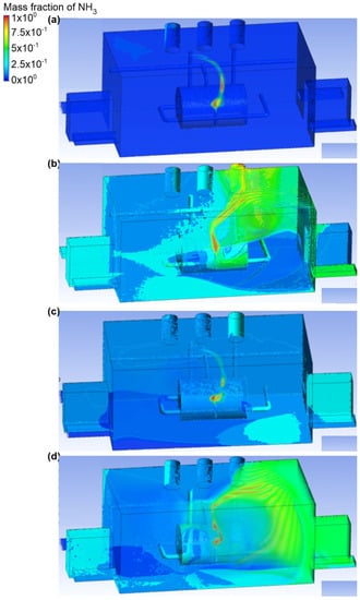
Figure 2.
Ammonia distribution in the engine room for: (a) scenario A, (b) scenario B, (c) scenario C, and (d) scenario D.
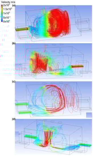
Figure 3.
Velocity distribution in the engine room for: (a) scenario A, (b) scenario B, (c) scenario C, and (d) scenario D.
The second variant included ammonia outflow from the top connector no. 1, active exhaust chimney no. 2 (middle), and ammonia outflow rate (mass flow rate was equal to 0.1 kg/s) (Figure 4 and Figure 5). In scenario A, the air velocity at input no. 2 was equal to 2.4 m/s, and in the exhaust chimney it was around 1.4 m/s. Moreover, no gaseous ammonia flow to the exhaust chimney no. 2 and towards the inactive chimney no. 3 was observed. Ammonia was also found to be deposited in the corner of the building above entrance no. 2 (the mass fraction at this point was in the range of 0.2–0.4). In scenario B, turbulent air flow was recorded. As a result of this turbulence, ammonia in the initial stage of the ventilation operation did not appear in the exhaust chimney no. 2, but accumulated in the inactive chimney no. 1 (mass fraction 0.7). In addition, a cloud of ammonia was formed on the front wall of door no. 2 (mass fraction was in the range of 0.2–0.3). In Scenario C, the value of air velocity in input no. 1 and no. 2 was equal to 1 m/s, and in the exhaust, the chimney was equal to 1.5 m/s. Furthermore, air turbulence was observed to cause a large volume cloud of ammonia to move towards the active air inlets, but the mass fraction of the gas in this cloud was equal to 0.2. A large amount of ammonia (mass fraction in the range 0.3–0.4) was found in the exhaust chimneys no. 1 and no. 3, as well as in the engine room, where the air intakes were not active. Scenario D assumed that the building would be supplied with air through inlet no. 2 and no. 4. The air velocity in this scenario was equal to the velocity in scenario C. It was noticed that the ammonia cloud was moving towards active exhaust chimney no. 2, but also a large part of it with a mass fraction of approximately 0.4 spread to door no. 1 and door no. 2, thus, causing the release of gas throughout the building.
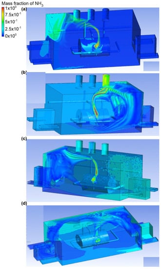
Figure 4.
Ammonia distribution in the engine room for: (a) scenario A, (b) scenario B, (c) scenario C, and (d) scenario D.
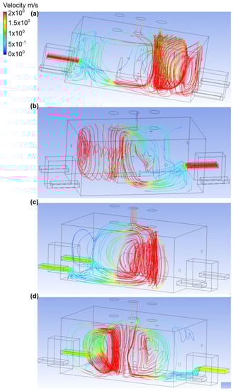
Figure 5.
Velocity distribution in the engine room for: (a) scenario A, (b) scenario B, (c) scenario C, and (d) scenario D.
The third variant assumed that the lower stub pipe was a place of ammonia outflow, and the gas outflow rate was equal to 0.1 kg/s. Moreover, the exhaust chimney no. 3 was active (Figure 6 and Figure 7). Scenario A assumes the inflow of air to the engine room through inlet no.2. The air speed at the inlet was equal to 2.3 m/s and at the outlet (exhaust chimney no. 3) was equal to 1.5 m/s. In addition, the largest mass share of ammonia in scenario A was observed in the gas tank (approximately 0.8). Furthermore, it was noticed that, in the whole engine room (except for air flow places), there was a mass fraction of ammonia in the range of 0.1–0.2. In scenario B, the air into the building was supplied through inlet no. 4. The velocity of the air was the same as in scenario A. In this case, the ammonia cloud became large in the tank (mass fraction of about 0.7) and the cloud moved towards the wall with an active air inlet. The mass fraction of ammonia at this point was in the range of 0.3–0.4, while in the entire building it was approximately 0.2. Scenario C assumes the air inflow to the engine room through inlet no. 2 and inlet no. 1. The air velocity at each of the inlets was equal to 1.2 m/s, and at the exhaust, the chimney was equal to approximately 1.4 m/s. Moreover, it was recorded that the released gas cloud received the largest volume immediately after release. The cloud then moved to the wall behind the tank, and the mass fraction in the cloud ranged from 0.9 at the outlet to 0.3 at the wall. Furthermore, in the entire building, the mass fraction of ammonia was in the range 0.1–0.2. In scenario D, inlet no. 2 and inlet no. 4 were active air inlets to the building. The mass fraction in the cloud ranged from 0.9 at the outlet to 0.3 at the wall. In the entire engine room, the mass fraction of the gas was in the range 0.1–0.2. The probable cause of the spread of ammonia throughout the building, both in simulation 3 and in previous simulations, was air turbulence.
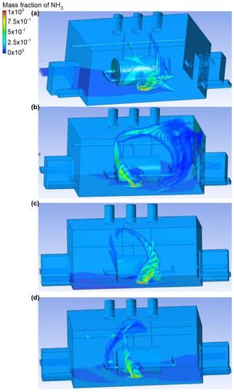
Figure 6.
Ammonia distribution in the engine room for: (a) scenario A, (b) scenario B, (c) scenario C, and (d) scenario D.
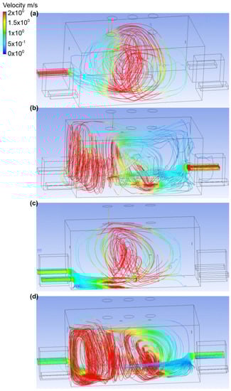
Figure 7.
Velocity distribution in the engine room for: (a) scenario A, (b) scenario B, (c) scenario C, and (d) scenario D.
The fourth variant analyzed assumed that the bottom connector was a place of ammonia outflow. The gas outflow rate was equal to 0.1 kg/s and the exhaust chimney no. 2 was active (Figure 8 and Figure 9). In scenario A, the air flow occurred through inlet no. 2. The air flow velocity at the inlet was equal to 2.4 m/s, and at the outlet was in the range 1.5–1.6 m/s. Moreover, it was observed that in this case, the ammonia, when released, formed into a small cloud, which was directed towards the active exhaust stack. The mass fraction of ammonia was also recorded in the entire building (excluding the airflow zone in the range of 0–0.1). In scenario B, the air was supplied from inlet no. 4. The air flow velocity was the same as in scenario A. In this scenario, most of the gas released along with the flowing air went to the active exhaust stack, while the amount of gas distributed throughout the engine room was in the range of 0–0.1. Scenario C assumed that the engine room was supplied with air through inlet no. 1 and inlet no. 2. The air flow velocity at each of the inlets was equal to 1.1 m/s, and in the exhaust stack it was nearly 1.5 m/s. Furthermore, it was recorded that the main portion of ammonia (mass fraction equal to 0.4) occurred in the gas tank and on the wall behind the tank. In the part of the building with inactive air inlets, the mass fraction of ammonia oscillated around 0.1. Scenario D assumes the airflow to the engine room through inlet no. 1 and inlet no. 4. The air velocity was the same as in scenario C. It was observed that, after release, ammonia went directly to the active exhaust chimney no. 2, but also a large part of the gas spread in the ceiling zone at inlet no. 1 and near the exhaust chimney no. 3. Ammonia was also observed in door no. 1. In the whole building, the mass fraction of ammonia was in the range of 0–0.1.
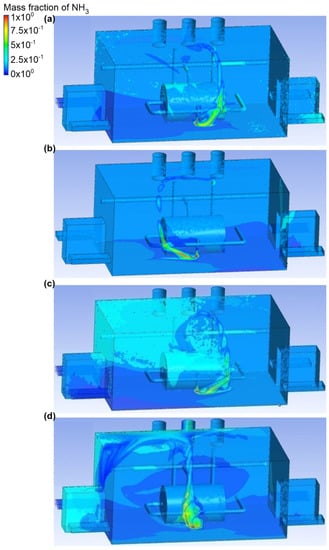
Figure 8.
Ammonia distribution in the engine room for: (a) scenario A, (b) scenario B, (c) scenario C, and (d) scenario D.
Figure 9.
Velocity distribution in the engine room for: (a) scenario A, (b) scenario B, (c) scenario C, and (d) scenario D.
The fifth variant analyzed assumed a different number of active exhaust chimneys (Figure 10 and Figure 11). First, it was assumed that the place of the ammonia outflow was the upper connector (outflow no. 1), and the rate of ammonia outflow was equal to 0.1 kg/s. Moreover, the exhaust chimney no. 1 and the exhaust chimney no. 3 were active. In scenario A, the air inflow to the engine room occurred through inlet no. 2. The inlet air velocity was equal to 2.2 m/s. In exhaust chimney no. 3, it was equal to 0.5 m/s, and in exhaust chimney no. 1, it was equal to 1 m/s. In addition, a large portion of ammonia was observed with a mass fraction of 0.4–0.5 in the wall at inlet no. 3 and no. 4, and on the wall opposite the gas tank. After being released, the ammonia cloud was directed towards the active exhaust chimney no. 3, but a large part of it did not end up in the chimney. The gas accumulated at the wall with inlet no. 2, and its mass fraction at this point fluctuated around 0.2–0.3. In scenario B, the active air inlet was inlet no. 3. The air flow velocity was the same as in scenario A. It was noticed that, in this case, the released ammonia went directly to the exhaust chimney no. 3. Scenario C assumes the inflow of air to the engine room through inlet no. 3 and no. 4. The air flow velocity at each of the inlets was equal to 1.3 m/s. In exhaust chimney no. 3, it was equal to 0.7 m/s, although in exhaust chimney no. 1 it was equal to 0.9 m/s. Moreover, it was recorded that, in scenario C, the gas after release behaved as in the previous scenario (i.e., it flowed towards exhaust stack no.1). Furthermore, ammonia also spread to other areas of the building, near chimney fan no. 1 (the mass fraction of ammonia was in the range of 0.1–0.2). Scenario D assumed that the air inlet to the engine room occurred through inlet no. 2 and inlet no. 3. The air flow velocity at the inlet in scenario D was the same as in scenario A, and in the case of the outlets, exhaust chimney no. 1 was equal to 0.8 m/s, and chimney lift no. 3 was equal to 0.6 m/s. Ammonia clearly moved towards exhaust chimney no. 1. In most parts of the building, the mass fraction of gas fluctuated in the range of 0.1–0.2.
Figure 10.
Ammonia distribution in the engine room for: (a) scenario A, (b) scenario B, (c) scenario C, and (d) scenario D.
Figure 11.
Velocity distribution in the engine room for: (a) scenario A, (b) scenario B, (c) scenario C, and (d) scenario D.
In the sixth variant, it was assumed that the upper connector was a place of ammonia outflow. Furthermore, the gas outflow rate was equal to 0.1 kg/s, and the active exhaust chimney no. 2 and exhaust chimney no. 3 (Figure 12 and Figure 13). Scenario A assumed that air was supplied to the building through inlet no. 1. Furthermore, the air flow velocity at the inlet was equal to 2.2 m/s. In exhaust chimney no. 3, it was equal to 0.3 m/s, and in exhaust chimney no. 2, it was equal to 1.2 m/s. It was observed that, in this scenario, after being released, ammonia formed into a cloud and stayed near the wall at active inlet no. 1. An important observation was also the fact that ammonia occupied the entire volume of the object, and its mass share was in the range of 0.4–0.5. In scenario B, air flowed into the building through inlet no. 4. The inlet air flow velocity was the same as in scenario A. In the exhaust chimney no. 3, it was equal to 0.9 m/s, and in the exhaust chimney no. 2, it was equal to 0.6 m/s. In scenario B, it was observed that when released, the ammonia formed a considerable cloud, most of which was concentrated at the wall at inlet no. 3. The mass fraction of ammonia in this cloud at the inactive chimney no. 3 was equal to 0.7, while on the wall itself it fluctuated around 0.3–0.5. In scenarios C and D, the air inlet occurred through, respectively, inlet no. 3 and inlet no. 4, and inlet no. 3 and inlet no. 2. The air flow velocity at each inlet was equal to 1.2 m/s, while at the outlets in both scenarios this value was, respectively, for exhaust chimney no. 3, equal to 1 m/s, and for exhaust chimney no. 2, equal to 0.7 m/s. It was recorded that the ammonia cloud spread towards the wall near door no. 2, and there was also an accumulation of gas with a mass fraction in the range of 0.2–0.4, as well as in the ceiling zone around the inactive exhaust chimney no. 1. It was also observed that in scenario C, large amounts of ammonia were deposited at door no. 1, and in inactive inlets no. 1 and no. 2.
Figure 12.
Ammonia distribution in the engine room for: (a) scenario A, (b) scenario B, (c) scenario C, and (d) scenario D.
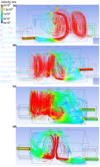
Figure 13.
Velocity distribution in the engine room for: (a) scenario A, (b) scenario B, (c) scenario C, and (d) scenario D.
In the seventh variant, it was assumed that the bottom connector was the place where ammonia was released. Furthermore, the discharge no. 2 was the discharge of gases, and its rate was equal to 0.1 kg/s. Furthermore, the active exhaust was chimney no.1 and chimney no. 3 (Figure 14 and Figure 15). In scenario A, air was supplied to the building through inlet no. 1. Inlet air velocity was equal to 2.5 m/s. At outlet no. 3, it was equal to 0.3 m/s, and at outlet no. 1 it was equal to 1.3 m/s. It was observed that the ammonia in the initial phase after its release collected under the tank, and then the gas cloud increased and concentrated on the wall behind the tank throughout the engine room. The mass fraction of ammonia at this point was approximately equal to 0.4. In scenario B, the inflow of air through the inlet no. 3 was assumed. In this case, the air velocity at the inlet was the same as in the case of scenario A, and in exhaust chimneys no. 3 and no. 1 it was equal to 0.9 m/s and 0.6 m/s, respectively. Furthermore, ammonia was recorded to be concentrated mainly in the tank, and a small amount of it spread throughout the engine room (mass fraction approximately equal to 0.1). In scenario C, inlet no. 3 and inlet no. 4 were active air inlets into the building. The air flow velocity at each inlet was equal to 1.2 m/s, while in the exhaust chimneys no. 3 and no. 1 it was equal to 1.1 m/s and 0.5 m/s, respectively. Furthermore, it was observed that, in scenario C, the ammonia release was directed towards the active exhaust chimney no. 1, but also spread throughout the building. The mass fraction of ammonia on the wall with inlet no. 3 and no. 4 was approximately equal to 0.3. In the entire engine room, it fluctuated in the range of 0.2–0.3. In scenario D, the air flow did not occur through inlets no. 2 and no. 3. The air flow velocity at the inlet was the same as in scenario C, and in the exhaust air chimneys it was approximately equal to 1 m/s. Moreover, it was noticed that the gas cloud was concentrated in the center of the building above the ammonia tank. It was noted that a small amount of gas was deposited in the corner of the room at inlet no. 4 and in door no. 2.
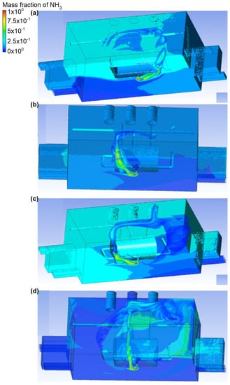
Figure 14.
Ammonia distribution in the engine room for: (a) scenario A, (b) scenario B, (c) scenario C, and (d) scenario D.
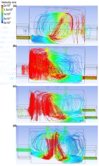
Figure 15.
Velocity distribution in the engine room for: (a) scenario A, (b) scenario B, (c) scenario C, and (d) scenario D.
In the eighth variant, it was assumed that the bottom connector was a place of ammonia release (outflow no. 2, ammonia outflow rate was equal to 0.1 kg/s). Moreover, the active exhausts were air chimneys no. 3 and no. 2 (Figure 16 and Figure 17). In scenario A, air was supplied through inlet no. 1. The air flow velocity at the inlet was equal to 2.2 m/s, and at the outlets no. 2 and no. 3 it was equal to 1 m/s and 0.5 m/s, respectively. Moreover, it was observed that, in scenario A, ammonia in the initial phase condensed under the tank, and then the gas moved towards the exhaust chimney no. 2. In the entire engine room, the mass fraction of ammonia fluctuated around 0.1. Scenario B assumes an airflow to the building through entry no. 3. The air flow velocity at the inlet was the same as in scenario A, and in the exhaust chimneys no. 2 and no. 3 it was equal to 0.3 m/s and 1.1 m/s, respectively. It was noticed that the gas, after the release, flowed towards exhaust chimney no. 2, and a small part of the cloud was concentrated in the inactive exhaust stack no. 1. In the whole building, as in scenario A, there was a mass fraction of ammonia within the limit of 0.1.
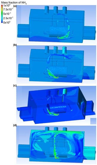
Figure 16.
Ammonia distribution in the engine room for: (a) scenario A, (b) scenario B, (c) scenario C, and (d) scenario D.
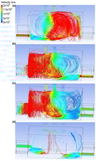
Figure 17.
Velocity distribution in the engine room for: (a) scenario A, (b) scenario B, (c) scenario C, and (d) scenario D.
Scenario C assumed that the air reached the building through inlet no. 3 and inlet no. 4. The air flow velocity at each of the inlets was equal to 1.2 m/s, and its value in the exhaust chimneys no. 2 and no. 3 was equal to 0.4 m/s and 1.1 m/s, respectively. The highest concentration of ammonia (small volume) occurred next to the gas tank. A small mass fraction of ammonia was recorded in exhaust chimney no. 1.
Scenario D assumes that air inflow to the engine room was through inlet no. 2 and inlet no. 3. The air flow velocity at the inlet was the same as in scenario C, while the value for the exhaust chimneys no. 2 and no. 3 was equal to 1 m/s at each of the outlets. Moreover, there was a lot of air turbulence, as a result of which the gas released spread throughout the building. Its largest mass share (approximately 0.6) was observed in the ceiling zone above the ammonia tank.
4. Discussion
The possibility of a leakage accident occurring at a large-scale causes concern. An important issue for the protection of human life and the environment is understanding the mechanisms of the release of toxic gases into the atmosphere. Research on the course of dispersion of individual gases allows prediction of the risk of a sudden release of toxic gas to a large extent. Kashi et al. investigated chlorine dispersion in an urbanized area. Similarly to the current study, the object that was recognized in the simulation as a source of chlorine release was a section of an industrial building, such as a water treatment plant []. Any analytical model which addresses all the factors that can influence the movement of gases throughout a building must deal with a complex set of interdependent factors []. Analyzing whether the model can describe the temporal spatial evolution of hazardous materials is critical to the assessment of model performance []. Numerical simulations in this paper were carried out for various variants, i.e., changing the initial air velocity in the inlet to the engine room and the air velocity in the ventilation hood, using a certain number of inlets and outlets during ventilation, and changing the place of the ammonia outflow.
A great number of factors determine the release of liquefied gas. To solve these problems, it is necessary to use numerical methods based on computational fluid dynamics codes (CFD codes) []. CFD simulations can be used to assess natural ventilation in a room by solving the interaction between urban wind flow and indoor airflow []. Numerical modeling of ammonia dispersion is related to the evaporation and emission of gases into the atmosphere []. Ammonia is an explosive-safe gas because it cannot be ignited with a match or a red-hot cigarette. Its ignition energy is 2000 times greater than that of hydrogen, and 20 times greater than that of hydrocarbons [].
Moreover, many CFD simulations work with different turbulence models; for example, the k-ε model, RNG model, k-ω (standard) model, shear stress transport (SST) model, etc., have each been carried out to reproduce the dense gas dispersion []. Galeev et al. observed that the k-ε model successfully reproduces the dispersion of dense gas in the atmosphere []. This was in line with the present study.
According to the received results, it would be recommended that:
- In-depth knowledge of the process of ammonia spreading in the ammonia engine room building is an important issue for the safety of employees of plants using ammonia in production processes, as well as for chemical and ecological rescue groups of the State Fire Service during the removal of the consequences of an event, which results in an emergency release of ammonia in a confined space.
- It is strongly recommended to ventilate the ceiling zone or inactivated exhaust chimneys due to the risk of ammonia build up.
- To prevent ammonia spreading after its release from the top and bottom stub pipe, the side ventilation ducts should be activated.
Limitations of the Study
The CFD model was used within the designated ammonia engine room. The following assumptions were made due to the type of simulation; the dimensions of the doors and ventilation openings in the front walls of the building have been modified. As a result of these changes, the doors and vents took the form of cuboids. In addition, the turbulence model, k-ε, was selected.
5. Conclusions
Fire safety engineering is recognized as a unique branch of engineering. When reviewing the needs of the building, there may be a number of objectives relevant to the fire strategy. An emergency ammonia leakage of 0.1 kg/s in the assumed air flow was observed to pose a great threat to the engineers in the engine room, because in many simulated scenarios ammonia was able to spread throughout the building. Regardless of the number of active air inlets and their location, the air stream often became turbulent, thus causing the released ammonia to concentrate in a large area of the ammonia engine room. In addition, ventilation was the most effective in two variants: with ammonia outflow from the upper connector, active inlet no. 2, and active exhaust chimney no. 3; and when ammonia flows from the lower connector, and air flows from inlet no. 3 and inlet no. 2, with active exhaust chimneys no. 2 and no. 3.
After being released, ammonia accumulated in the ceiling zone, and in inactive exhaust chimneys, air inlets, and doors. The effectiveness of ventilation depends on the number of active air vents and exhausts, as well as their distribution in the building.
Finally, the use of numerical methods in engineering practice allows for a quick and effective solution of the ventilation problem both in ammonia engine rooms and in the design of smoke exhaust systems for buildings, as well as for ventilation systems in collective housing buildings, without incurring additional research costs that would occur if the investigation was carried out in a physically existing facility.
The proposed manuscript presents a numerical approach to toxic gas dispersion in an office. The presented approach may help the with the planning of spatial distribution of a ventilation system’s elements, as well as its capacity. Furthermore, knowledge about toxic gas distribution, after the onset of a ventilation system, for the selected configuration can be helpful in planning the work of employees, as well as the possible evacuation routes of injured people.
Author Contributions
Conceptualization, Z.S.; methodology, Z.S.; software, Z.S. and A.P.; validation, A.P.-P., M.M.-L., W.R.-K. and A.D.; formal analysis, A.P. and A.P.-P.; investigation, Z.S.; resources, Z.S. and W.R.-K.; data curation, A.P.; writing—original draft preparation, A.P. and A.D.; writing—review and editing, A.P.-P. and Z.S.; visualization, Z.S.; supervision, Z.S. and A.P.; project administration, Z.S.; funding acquisition, Z.S. All authors have read and agreed to the published version of the manuscript.
Funding
This research received no external funding.
Institutional Review Board Statement
Not applicable.
Informed Consent Statement
Not applicable.
Data Availability Statement
Data is available on request from the corresponding author.
Conflicts of Interest
The authors declare no conflict of interest.
References
- Longxiang, D.; Hongchao, Z.; Liang, H.; Bin, Y.; Licheng, L.; Liyang, W. Simulation of heavy gas dispersion in a large indoor space using CFD model. J. Loss Prev. Process Ind. 2017, 46, 1–12. [Google Scholar]
- Rosa, A.C.; de Souza, I.T.; Terra, A.; Hammad, A.W.A.; Di Gregorio, L.T.; Vazquez, E.; Haddad, A. Quantitative risk analysis applied to refrigeration’s industry using computational modeling. Results Eng. 2021, 9, 100202. [Google Scholar] [CrossRef]
- Maliselo, P.S.; Nkonde, G.K. Ammonia Production in Poultry Houses and Its Effect on the Growth of Gallus Gallus Domestica (Broiler Chickens): A Case Study of a Small Scale Poultry House in Riverside, Kitwe, Zambia. Int. J. Sci. Technol. Res. 2015, 4, 141–145. [Google Scholar]
- Cao, G.; Awbi, H.; Yao, R.; Fan, Y.; Sirén, K.; Kosonen, R.; Zhang, J. A review of the performance of different ventilation and airflow distribution systems in buildings. Build. Environ. 2014, 73, 171–186. [Google Scholar] [CrossRef]
- Melikov, A.; Ivanova, T.; Stefanova, G. Seat headrest-incorporated personalized ventilation: Thermal comfort and inhaled air quality. Build. Environ. 2012, 47, 100–108. [Google Scholar] [CrossRef]
- Yassin, M.F. Experimental study on contamination of building exhaust emissions in urban environment under changes of stack locations and atmospheric stability. Energy Build. 2013, 62, 68–77. [Google Scholar] [CrossRef]
- Ang, G.; Jie, G.W.; Chiming, W.; Haibao, F. Numerical Simulation and Optimization Design of Ship Engine Room Ventilation System. Chin. J. Ship Res. 2014, 9, 93–98. [Google Scholar]
- Zhang, Z.; Zeng, L.; Shi, H.; Liu, H.; Yin, W.; Gao, J.; Wang, L.; Zhang, Y.; Zhou, X. CFD studies on the spread of ammonia and hydrogen sulfide pollutants in a public toilet under personalized ventilation. J. Build. Eng. 2022, 46, 103728. [Google Scholar] [CrossRef]
- Tung, Y.-C.; Hu, S.-C.; Tsai, T.-Y. Influence of bathroom ventilation rates and toilet location on odor removal. Build. Environ. 2009, 44, 1810–1817. [Google Scholar]
- Gai, W.-M.; Du, Y.; Deng, Y.-F. Regional evacuation modeling for toxic-cloud releases and its application in strategy assessment of evacuation warning. Saf. Sci. 2018, 109, 256–269. [Google Scholar] [CrossRef]
- Hannaa, S.R.; Hansenb, O.R.; Ichardb, M.; Strimaitis, D. CFD model simulation of dispersion from chlorine railcar releases in industrial and urban areas. Atmos. Environ. 2009, 43, 262–270. [Google Scholar] [CrossRef]
- Polanczyk, A.; Salamonowicz, Z. Computational modeling of gas mixture dispersion in a dynamic setup—2d and 3d numerical approach. E3S Web Conf. 2018, 44, 8. [Google Scholar] [CrossRef] [Green Version]
- Ziemińska-Stolarska, A.; Polańczyk, A.; Zbiciński, I. 3-D CFD simulations of hydrodynamics in the Sulejow dam reservoir. J. Hydrol. Hydromech. 2015, 63, 334–341. [Google Scholar] [CrossRef] [Green Version]
- Salamonowicz, Z.; Krauze, A.; Majder-Lopatka, M.; Dmochowska, A.; Piechota-Polanczyk, A.; Polanczyk, A. Numerical reconstruction of hazardous zones after the release of flammable gases during industrial processes. Processes 2021, 9, 307. [Google Scholar] [CrossRef]
- Wawrzyniak, P.; Podyma, M.; Zbiciński, I.; Bartczak, Z.; Polanczyk, A.; Rabaeva, J. Model of Heat and Mass Transfer in an Industrial Counter-Current Spray-Drying Tower. Dry. Technol. 2012, 30, 1274–1282. [Google Scholar] [CrossRef]
- Choi, J.; Hur, N.; Kang, S.; Lee, E.D.; Lee, K.-B. A CFD simulation of hydrogen dispersion for the hydrogen leakage from a fuel cell vehicle in an underground parking garage. Int. J. Hydrogen Energy 2013, 38, 8084–8091. [Google Scholar] [CrossRef]
- Chang, J.C.; Hanna, S.R. Air quality model performance evaluation. Meteorol. Atmos. Phys. 2004, 87, 167–196. [Google Scholar] [CrossRef]
- Sklavounos, S.; Rigas, F. Validation of turbulence models in heavy gas dispersion over obstacles. J. Hazard. Mater. 2004, 108, 9–20. [Google Scholar] [CrossRef]
- Xing, J.; Liu, Z.; Huang, P.; Feng, C.; Zhou, Y.; Zhang, D.; Wang, F. Experimental and numerical study of the dispersion of carbon dioxide plume. J. Hazard. Mater. 2013, 256–257, 40–48. [Google Scholar] [CrossRef]
- Chao, C.; Wei, T.; Liyan, L. Numerical simulation of water curtain application for ammonia release dispersion. J. Loss Prev. Process Ind. 2014, 30, 105–112. [Google Scholar]
- Polanczyk, A.; Salamonowicz, Z.; Majder-Lopatka, M.; Dmochowska, A.; Jarosz, W.; Matuszkiewicz, R.; Makowski, R. 3D Simulation of Chlorine Dispersion in Rrural Area. Annu. Set Environ. Prot. 2018, 20, 1035–1048. [Google Scholar]
- Gant, S.; Narasimhamurthy, V.; Skjold, T.; Jamois, D.; Proust, C. Evaluation of multi-phase atmospheric dispersion models for application to Carbon Capture and Storage. J. Loss Prev. Process Ind. 2014, 32, 286–298. [Google Scholar] [CrossRef] [Green Version]
- Pontiggia, M.; Derudi, M.; Alba, M.; Scaioni, M.; Rota, R. Hazardous gas releases in urban areas: Assessment of consequences through CFD modelling. J. Hazard. Mater. 2010, 176, 589–596. [Google Scholar] [CrossRef] [PubMed]
- Karin, H.; Jean-Marie, B.; Aurélia, D.; Gilles, D. Heavy gas dispersion by water spray curtains: A research methodology. J. Loss Prev. Process Ind. 2005, 18, 506–511. [Google Scholar]
- Kashi, E.; Mirzaei, F.; Mirzaei, F. Analysis of Chlorine Gas Incident Simulation and Dispersion within a Complex and Populated Urban Area Via Computation Fluid Dynamics. Adv. Environ. Technol. 2015, 1, 49–58. [Google Scholar]
- Yang, J.; Yang, Y.; Chen, Y. Numerical Simulation of Smoke Movement Influence to Evacuation in a High-Rise Residential Building Fire. Procedia Eng. 2012, 45, 727–734. [Google Scholar] [CrossRef] [Green Version]
- Labovsky, J.; Jelemensky, L. CFD simulations of ammonia dispersion using “dynamic” boundary conditions. Process Saf. Environ. Prot. 2010, 88, 243–252. [Google Scholar] [CrossRef]
- van Hoof, T.; Blocken, B. CFD evaluation of natural ventilation of indoor environments by the concentration decay method: CO2 gas dispersion from a semi-enclosed stadium. Build. Environ. 2013, 61, 1–17. [Google Scholar] [CrossRef]
- Galeev, A.; Starovoytova, E.; Ponikarov, S. Numerical simulation of the consequences of liquefied ammonia instantaneous release using FLUENT software. Process Saf. Environ. Prot. 2013, 91, 191–201. [Google Scholar] [CrossRef]
- Wei, T.; Dong, L.; Xiyan, G.; Huang, D.; Liyan, L.; Yang, W. Accident consequence calculation of ammonia dispersion in factory area. J. Loss Prev. Process Ind. 2020, 67, 104271. [Google Scholar]
- Gousseau, P.; Blocken, B.; van Heijst, G.J.F. CFD simulation of pollutant dispersion around isolated buildings: On the role of convective and turbulent mass fluxes in the prediction accuracy. J. Hazard. Mater. 2011, 194, 422–434. [Google Scholar] [CrossRef] [PubMed]
Publisher’s Note: MDPI stays neutral with regard to jurisdictional claims in published maps and institutional affiliations. |
© 2022 by the authors. Licensee MDPI, Basel, Switzerland. This article is an open access article distributed under the terms and conditions of the Creative Commons Attribution (CC BY) license (https://creativecommons.org/licenses/by/4.0/).