Article

Three-Dimensional Dynamic Variations of Ground/Air Surface Temperatures and Their Correlation with Large-Scale Circulation Indexes in Southwest China (1980–2019)

1
School of Geography and Ecotourism, Southwest Forestry University, Kunming 650224, China
2
Southwest Research Center for Eco-Civilization, National Forestry and Grassland Administration, Kunming 650224, China
3
National (Yunnan Province) Field Science Observation and Research Station Yulong Snow Mountain Cryosphere and Sustainable Development, Northwest Institute of Eco-Environment and Resources, Chinese Academy of Sciences, Lanzhou 730000, China
4
Faculty of Geography, Yunnan Normal University, Kunming 650500, China
*
Author to whom correspondence should be addressed.
Atmosphere 2022, 13(7), 1031; https://doi.org/10.3390/atmos13071031
Submission received: 28 May 2022 / Revised: 21 June 2022 / Accepted: 25 June 2022 / Published: 28 June 2022
(This article belongs to the Topic Climate Change and Environmental Sustainability)

Abstract

:
Air/soil temperatures play important roles in land–atmosphere interactions. The three-dimensional (temporal, spatial, and vertical) variations of maximum, mean, and minimum ground soil temperature at 0 cm (GSTx, GSTm, and GSTn, respectively), surface air temperature at 2 m (SATx, SATm, and SATn, respectively), and soil–air temperature difference (SATDx, SATDm, and SATDn, respectively) and their potential linkages with large-scale indexes in Southwest China during 1980–2019 were analyzed. Variations of GST and SAT at the majority of stations (pixels) exhibited significant (p ≤ 0.05) warming, albeit at different rates; consequently, SATD exhibited different variation. Moreover, the period of GST, SAT, and SATD was similar in intra-annual and interannual oscillation but was different in interdecadal oscillation. The variation rate of GST, SAT, and SATD exhibited significant (p ≤ 0.05) correlation with elevation, but with different variation gradient. Notably, asymmetric variation of SATDx (downward trend) and of SATDn (upward trend) with elevation was found at elevations >3 km. Wavelet coherence showed that the Atlantic Multidecadal Oscillation is the dominant factor affecting GST and SAT, whereas the Pacific Decadal Oscillation and the North Atlantic Oscillation make the greatest contributions to SATD. It was found that GST, SAT, and SATD exhibit different variations under the effects of global warming, the driving mechanism of which requires further study.

1. Introduction

The connection between soil and air temperatures is one of the fundamental aspects of land–atmosphere interactions [1,2,3,4]. In such interactions, although soil temperature is different from air temperature in terms of value, oscillation [5], and variation trend [6], the two parameters are normally closely coupled. Previous research has investigated both the fluctuation of soil temperature at different depths [3,7,8,9,10] and the relationship between soil temperature and air temperature [11,12,13,14]. However, this study focused on soil temperature measured at a depth of 0 cm, i.e., ground soil temperature (GST), and surface air temperature (SAT) because the difference between GST and SAT (i.e., SATD) is proportional to the surface sensible heat flux [15,16], which has substantial influence on soil microorganisms [17], vegetation [18], and climate [14,19]. Meanwhile, under the background of global warming, GST has been found to differ from SAT in terms of its variation [1,6] and trend [2,7,20]. Therefore, because surface temperature has been and will be accompanied by widespread change in this context [21], revealing the different variations of GST-, SAT-, and SATD-related indexes and their responses to climate change is of great importance for understanding land–atmosphere interactions and energy exchange.
In recent years, GST, SAT, and SATD have been the subject of some research in China. For instance, He and Wang discovered that the multiyear national average GST and SAT lapse rate were comparable (i.e., 0.53 °C/100 m) [22]. Using the detrended fluctuation analysis method, Jiang et al. found that GST appears more sensitive for detecting persistent temperature change in comparison with SAT [11]. According to Wang et al., the rate of warming of GST in northern China is higher than that in southern regions [23]. Subsequently, Liao et al. reported that the maximum SATD occurs in China during the rainy season, which is compatible with the annual distribution of solar radiation [20]. Additionally, SATD has been found to exhibit a clearer trend of increase in northern regions of China than in southern regions [2]. Zhang et al. revealed that SAT and GST have a lagged correlation that is affected by snow cover [3]. The SATD on the Tibetan Plateau has been shown to present variation with periodicity of approximately 2 years [14]. Recent research has found that GST exhibited a significant rate of warming of 0.071 °C/year during 1983–2013 [24], which has increased from the rate of 0.047 °C/year during 1960–2014 [25].
The above research has revealed the spatiotemporal variation in air and ground temperatures in China, as well as possible causes. However, such analysis was concerned primarily with the spatiotemporal pattern of variation. Owing to elevation-dependent warming, the rate of warming of SAT incorporates an elevation gradient that reflects the fact that high-elevation regions experience more rapid change than low-elevation regions [26,27,28,29,30,31]. Therefore, it is important to ascertain whether the GST and SATD are consistent with the SAT that exhibits elevation gradient variation. Additionally, other earlier studies revealed the influence of precipitation [24,32], wind [33], snow depth [4,15,34,35,36], sunshine duration [37], and soil moisture [38] on air and ground temperatures. However, the average climatic temperature is closely governed by large-scale atmospheric circulation patterns [39]. Temperature change is affected by external forcing and by internal variability of the climate system [40,41]. The internal variability of the climate system includes the El Niño–Southern Oscillation (ENSO), North Atlantic Oscillation (NAO), Arctic Oscillation (AO), Pacific Decadal Oscillation (PDO), and Atlantic Multidecadal Oscillation (AMO), and it has significant effects on global and regional temperature [42,43,44,45]. However, few studies have investigated the potential associations of SAT, GST, and SATD with large-scale circulation indexes from the perspective of multiscale coherence.
Southwest China (SWC) has complex topography and is subject to substantial regional/local climate change [46]. However, the characteristics of GST, SAT, and SATD in SWC remain poorly understood, and further scientific research is needed. In this study, SWC was selected as the study area. Because there is lack of availability of meteorological observations from high-elevation regions in SWC, i.e., where elevation is >4000 m, daily observed data from regional meteorological stations were interpolated using a digital elevation model (DEM) into a raster with 1 km resolution using an ensemble of six algorithms (i.e., boosted regression tree, neural network, generalized additive model, multivariate adaptive regression spline, support vector machine, and random forest) to reveal the three-dimensional variation of SAT, GST, and SATD. Following Ma et al. [47], three-dimensional variation is defined as the spatiotemporal and vertical variation of GST-, SAT-, and SATD-related indexes in this study. Furthermore, wavelet transform coherence (WTC) was used to reveal potential linkages between GST, SAT, SATD, and the large-scale indexes.
The structure of the remainder of this paper is as follows. Section 2 introduces the study area, data sources, and methods used. Section 3.1 presents the three-dimensional variation of SAT, GST, and SATD, while Section 3.2 reveals potential linkages between SAT, GST, SATD, and the large-scale indexes. Section 4 and Section 5 provide a discussion based on the results of the study and state the derived conclusions, respectively. The objective of this paper was to attempt to answer the following two questions. (1) What were the characteristics of the three-dimensional variation of GST, SAT, and SATD in SWC during 1980–2019? (2) What potential linkages existed between GST, SAT, SATD, and the large-scale circulation indexes during 1980–2019?

2. Study Area, Data, and Methods
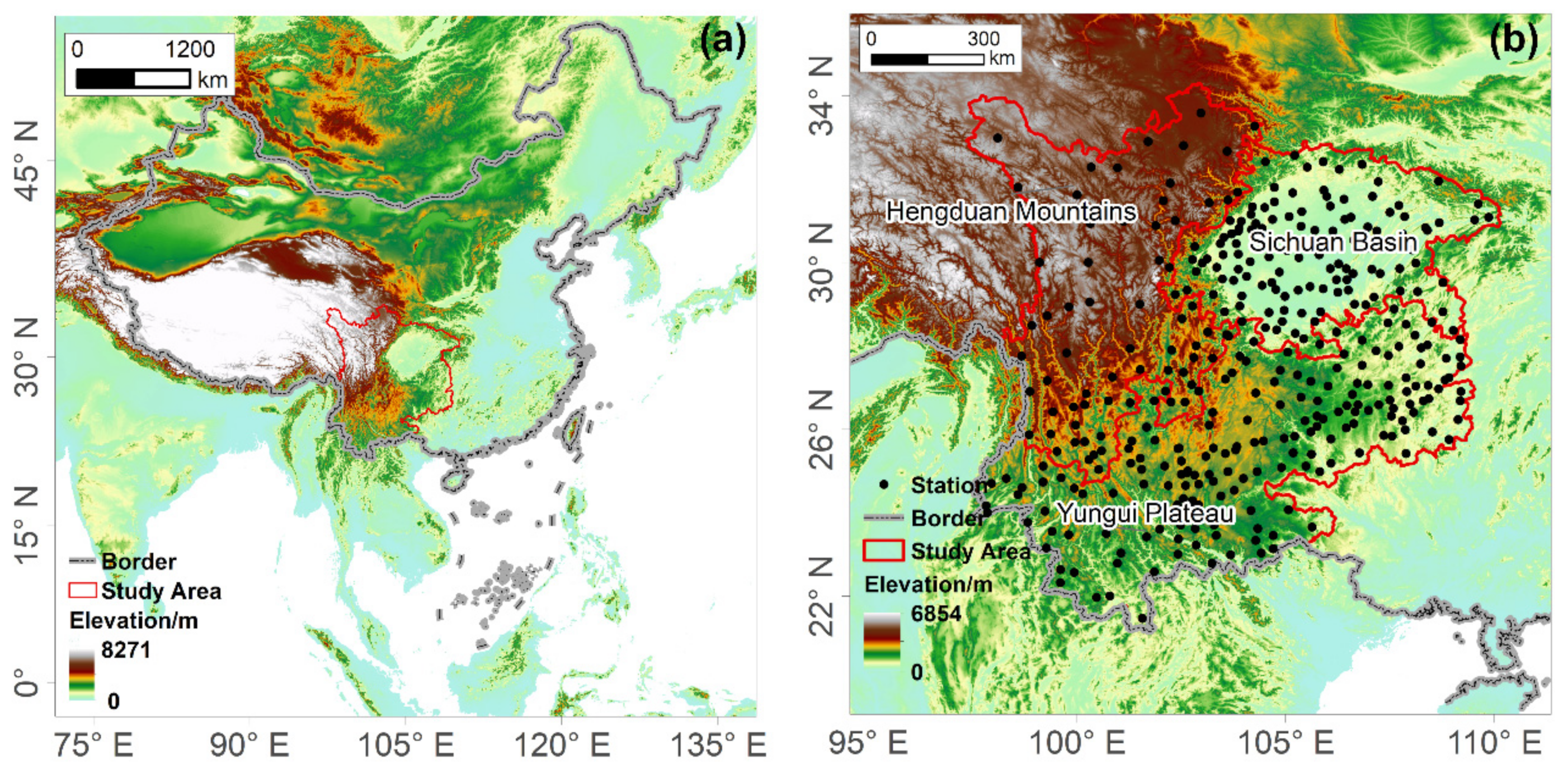
2.1. Study Area

The study area covers the geographical region of 20°54′–34°19′ N, 97°21′–112°4′ E (Figure 1). It extends across the transition zone from the first ladder to the second ladder of terrain in China, with average elevation of 2906 m and a relative elevation difference of 6854 m. The terrain elevation difference is large, and the landform types are complex. From the southeast to the northwest, the region is affected by tropical monsoon, subtropical monsoon, and plateau monsoon climates. Under the alternating influence of these different monsoon climate types, heat and precipitation are abundant. Annual average temperature is between −2.8 and 23.9 °C, annual cumulative precipitation is 54.6–2675.6 mm, annual average relative humidity is 46.6–85.0%, and the annual cumulative number of sunshine hours is 844–2531 h. Owing to the complex terrain and the characteristics of the monsoon circulations, there is substantial spatial difference in terms of the impact of climate change. Therefore, the study area was divided into three subareas, i.e., the Hengduan Mountains (HDM), Yungui Plateau (YGP), and Sichuan Basin (SCB).

2.2. Data Resources and Quality Control

Daily mean, maximum, and minimum data of SAT and GST observed at 400 meteorological stations were obtained from the China Meteorological Data Sharing Service System of the National Meteorological Information Center V3.0 (http://www.nmic.gov.cn/ (accessed on 31 December 2019)). Considering the quality of the data, the fact that for GST there exists large errors before 1980, and due to the requirement for additional stations for training during the interpolation process, we mainly concentrated on the period 1980–2019. However, for various natural and human/instrument-related reasons, the data set contained certain missing or erroneous values. Therefore, we discarded data from any station that had missing values for a period longer than five consecutive days. Ultimately, data from 368 out of the original 400 stations (67, 182, and 119 stations in HDM, YGP, and SCB) were selected for use in this study. Any further gaps in the data set were filled by applying linear regression between the elevation and data from surrounding stations that were within a 50 km diameter circle centered on the target meteorological station. The observed data were interpolated into a raster with 1 km resolution using the DEM and the R Machisplin package. Furthermore, nine GST-, SAT-, and SATD-related indexes were calculated (Table 1). The 1 km resolution DEM was derived from the Geospatial Data Cloud of China (http://www.gscloud.cn/ (accessed on 31 December 2019)). Additionally, six large-scale indexes (i.e., the AO, AMO, Multivariate ENSO Index (MEI), NAO, PDO, and Pacific/North American (PNA) teleconnection) were adopted to reveal potential linkages with the GST-, SAT-, and SATD-related indexes. The AO, AMO, PDO, NAO, and PNA indexes were derived from the National Oceanic and Atmospheric Administration Physical Sciences Laboratory website (https://psl.noaa.gov/data/climateindices/ (accessed on 31 December 2019)), while the MEI was derived from http://www.esrl.noaa.gov/psd/enso/mei/index.html (accessed on 31 December 2019).

2.3. Methodology

2.3.1. Data Interpolation

The observed data from the meteorological stations were interpolated into a raster with 1 km resolution using an ensemble of up to six algorithms (i.e., boosted regression tree, neural network, generalized additive model, multivariate adaptive regression spline, support vector machine, and random forest). During model tuning, each algorithm was systematically weighted from 0–1, and the fit of the ensemble model was evaluated. The best-performing model was determined via k-fold cross-validation (k = 10), and the model with the lowest residual sum of squares and lowest AIC (Akaike information criterion) of the test data was selected. Finally, the residuals were further calculated and interpolated using thin-plate-smoothing splines, which secondarily corrected the final ensemble model. However, if the R2 value of final correction was greater than the R2 value of the ensemble, the final correction was discarded. For example, multiyear averaged GST- and SAT-related indexes were interpolated by the six algorithms. The weights and R2 values of the GST- and SAT-related index interpolation results are presented in Table 2.

2.3.2. Extraction in Different Elevation Bins

Elevation was divided into 500 m bins to detect the elevation-dependent variation in SWC and the subareas. For example, for the 1000–1500 m bin, the variation rate of the stations and pixels in the bin was calculated. Then, the linear regression between the variation rate of each bin and elevation was used to quantify the elevation-dependent variation. The numbers of stations and pixels included in each of the bins are shown in Figure 2.

2.3.3. Other Methods

The modified Mann–Kendall test [48,49] and the moving mean difference method [49] are used to detect the significance of trends and to identify climate jump in time series. Moreover, ensemble empirical mode decomposition can decompose time series into intrinsic mode functions (IMFs) that can represent the oscillation of the original time series on a specific timescale [50,51]. Following Qian et al., the variance contribution rate was determined to assess the relational importance of each IMF component [52]. Furthermore, WTC was used to reveal potential linkages between the GST-, SAT-, and SATD-related indexes and the large-scale indexes [53]. WTC is based on the continuous wavelet transform [54], and it is a correlation coefficient in time–frequency space that can be used to quantify the relationship between two nonstationary series [55]. In contrast to WTC, multi-wavelet coherence (MWC) can determine the optimal factors and reveal their relationship [55,56]. In MWC, the percentage area of significant coherence (PASC) is used to quantify the explanation attributable to a particular predictor factor. When adding a particular predictor factor, if the associated PASC increases by at least 5%, then the particular predictor factor can be considered credible [57]. For WTC and MWC, the Monte Carlo approach (1000 count) based on a red noise background can be used to calculate the significance level. Additionally, global coherence can be used to evaluate the correlation between two time series at different scales, while neglecting the influence of time [58,59].

3. Results

3.1. Three-Dimensional Variation of Each Index

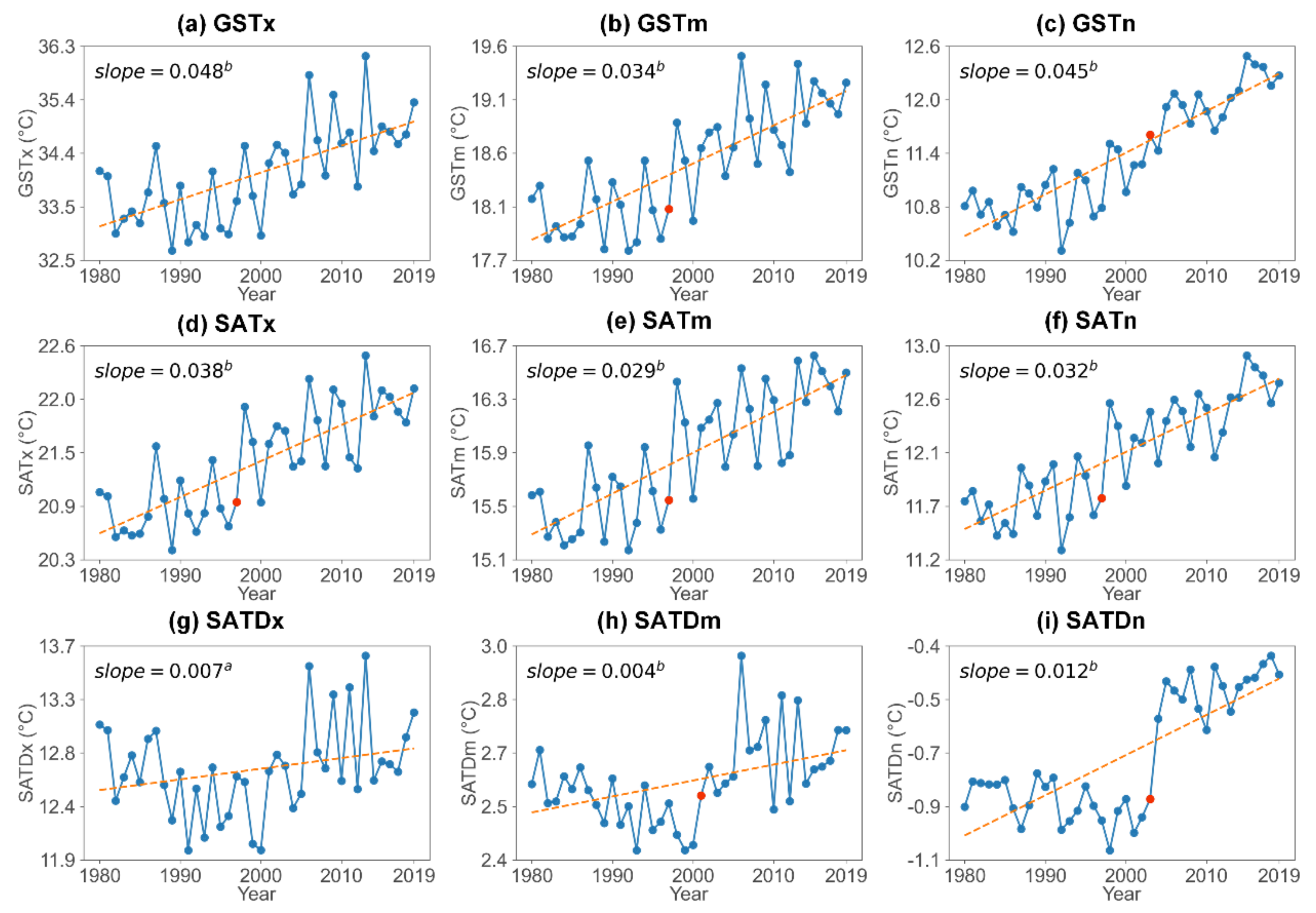
3.1.1. Temporal Trend

The trends and climate jump of the regional annual averaged GST-, SAT-, and SATD-related indexes in SWC are illustrated in Figure 3, and details of the seasonal averaged GST-, SAT-, and SATD-related indexes are summarized in Table 3. Additionally, the variation rate and climate jump of the annual and seasonal averaged GST-, SAT-, and SATD-related indexes of the subareas are presented in Tables S1 and S2, respectively. On an annual timescale, the regional annual averaged time series (1980–2019) of GST- and SAT-related indexes all show significant (p ≤ 0.01) warming in SWC (Figure 3a–f) and the subareas (Table S1). In addition to GSTx in HDM, the warming rates of the GST-related indexes are greater than those of the SAT-related indexes (Table S1). Consequently, the regional annual averaged SATD-related indexes exhibit an upward trend in SWC and the subareas, but the regional averaged SATDx exhibits a decreasing trend in HDM (Figure 3g–i and Table S1). The regional annual averaged SATDx and SATDn show the converse variation in HDM. Moreover, the regional annual averaged GST-, SAT-, and SATD-related indexes (except GSTx and SATDx) show a significant (p ≤ 0.05) climate jump between 1997 and 2003 (Figure 3 and Table 3). On the seasonal timescale, apart from the trends of decrease in HDM in the summer, autumn, and winter averaged SATDx of −0.005, −0.007, and −0.009 °C/year (p ≤ 0.05), respectively, the seasonal averaged GST-, SAT-, and SATD-related indexes all show a significant (p ≤ 0.05) trend of warming (Table 3 and Table S1). The fastest rates of warming of the regional averaged GST- and SAT-related indexes in SWC and the subareas (except in HDM) are found in spring (Table 3 and Table S1). Consistent with the climate jump on the annual timescale, the regional seasonal averaged GST-, SAT-, and SATD-related indexes in SWC and the subareas also show a climate jump between 1997 and 2004. However, a climate jump of the regional seasonal averaged GSTx is not evident in any season in the subareas (Table S2).

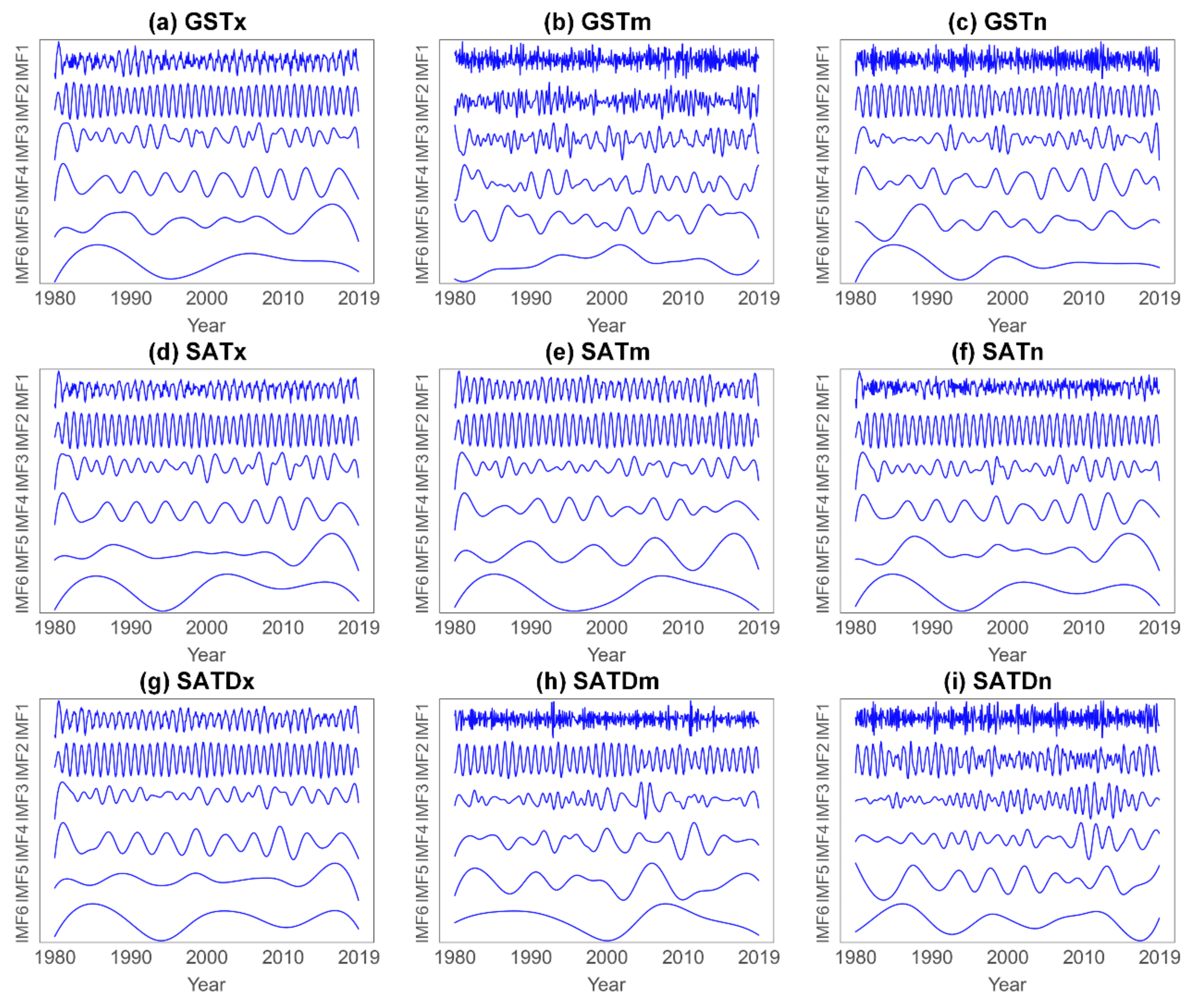
3.1.2. Periodic Analysis

The ensemble empirical mode decomposition of the regional monthly averaged GST, SAT-, and SATD-related indexes in SWC is illustrated in Figure 4, and Table 4 presents the period and variance contribution rate of each IMF in SWC. Additional details of the period and variance contribution of the regional monthly averaged GST-, SAT-, and SATD-related indexes in the subareas are presented in Table S3. As shown in Figure 4, the regional monthly average of the GST-, SAT-, and SATD-related indexes can be decomposed into six IMFs: intra-annual oscillation mode (IMF1 and 2), interannual oscillation mode (IMF3–5), and interdecadal oscillation mode (IMF6) (Figure 4). The IMF1 oscillation of the regional monthly averaged GST-, SAT-, and SATD-related indexes of SWC and the subareas is concentrated on 0.2–0.5 years (Table 4 and Table S3). Specifically, the period of the regional monthly averaged SAT is greater than that of the GST (Table 4 and Table S3). For IMF2, except for the regional monthly averaged GSTm and SATDn that have low-frequency oscillations of 0.2 and 0.6 years (except SATDn in SCB), respectively, the other indexes exhibit 1-year oscillation, and the variance contribution rate reaches 80% (Table 4 and Table S3). For the interannual oscillation mode, the dominant IMF oscillation of the regional monthly averaged GST-, SAT-, and SATD-related indexes in SWC and the subareas is IMF3 (oscillation: 1–2 years), which has the greater variance contribution in comparison with that of both IMF4 and IMF5. The oscillation of IMF4 and IMF5 is 2–9 years, which is similar to the 2–7-years period of an ENSO event. From the above, it can be determined that GST also exhibits a shorter period than SAT in terms of the interannual oscillation mode (Table 4 and Table S3). For the interdecadal oscillation mode, except for IMF6 of the regional monthly averaged SATDn in HDM and GSTn in YGP that show oscillation of 10.14 years, consistent with the period of sunspot activity (i.e., 11 and 23.41 years), the other indexes show low-frequency oscillation of near 14–23 years (Table 4 and Table S3). However, the period of IMF6 in the subareas shows considerable difference (Table S3). For example, the IMF6 period of GSTm is 10.7, 11.9, and 14.1 years in HDM, YGP, and SCB, respectively. Overall, the periods of the regional monthly averaged GST-, SAT-, and SATD-related indexes in SWC and the subareas are similar in terms of high-frequency oscillation (IMF1–3) and different in terms of low-frequency oscillation (IMF4–6).

3.1.3. Spatial Variation

Box-and-whisker plots of the annual averaged GST, SAT, and SATD variation rate of the observations during 1980–2019 are shown in Figure 5, and the seasonal variation rates of the observations are shown in Figure S1. From the boxplot figures, it can be seen that for the majority of stations the variation rate of the observed annual/seasonal averaged GSTx shows obvious fluctuation in comparison with the variation rate of the observed annual/seasonal averaged SATx and SATDx (Figure 5 and Figure S1). Moreover, it can be seen that the annual/seasonal averaged GST-, SAT-, and SATD-related indexes of the majority of observations exhibit increasing trends, and that the annual/seasonal averaged GST variation rate is greater than the variation rate of the annual/seasonal averaged SAT-related indexes (except GSTm in summer) (Figure 5 and Figure S1). To investigate the spatiotemporal pattern, the monthly and annual observed GST and SAT were interpolated into a 1 km resolution raster, as described in Section 2.3.1, and SATD was calculated by subtracting the SAT raster from the GST raster. Then, the variation rate at each pixel was calculated using the modified Mann–Kendall test (retaining only those pixels that satisfied the condition p ≤ 0.05).
The distribution of the spatial variation rate and the distribution of the interval of the annual averaged GST-, SAT-, and SATD-related indexes are shown in Figure 6, and the distribution of the seasonal variation rate and the distribution of the interval of each index are shown in Figures S2–S5. Meanwhile, the percentages of stations and pixels in SWC with significant (p ≤ 0.05) positive/negative trends of the annual/seasonal averaged GST-, SAT-, and SATD-related indexes are summarized in Table 5 and Table 6, respectively. Table S4 presents the percentages of stations with significant (p ≤ 0.05) increasing/decreasing trends in annual/seasonal averaged GST-, SAT-, and SATD-related indexes, and the percentages of pixels with significant (p ≤ 0.05) increasing/decreasing trends in annual/seasonal averaged GST-, SAT-, and SATD-related indexes in the subareas are presented in Table S5.
On the annual timescale, more than 90% of the stations and pixels in SWC exhibit a significant (p ≤ 0.05) trends of increase in the annual averaged SAT- and GST-related indexes (except GSTx) (Table 5 and Table 6). However, there is huge difference in the percentages of the stations and pixels with a significant (p ≤ 0.05) trend of increase between the annual averaged GSTx and SATx, for which nearly 30% of stations and pixels show the opposite trend (Table 5 and Table 6). For annual averaged SATD-related indexes, fewer than 50% of stations and pixels of the annual averaged SATDx and SATDm show significant (p ≤ 0.05) trends of increase, while approximately 78% of stations and 55% of pixels of the annual averaged SATDn exhibit significant (p ≤ 0.05) trends of increase (Table 5 and Table 6). However, although the majority of annual averaged GST- and SAT-related indexes exhibit trends of increase, there is difference in the variation rate between the annual averaged GST- and SAT-related indexes. Consequently, half the stations/pixels of the annual averaged SATD-related indexes show trends of increase, while the others exhibit decreasing trends. The variation rate of the annual averaged GSTx, GSTm, and GSTn is mainly in the range of 0.03–0.06 °C/year (i.e., 44%, 47%, and 58% of pixels, respectively) (Figure 6a–c). Consistent with the variation rate of most of the annual averaged GST-related indexes, the variation rate of SATx, SATm, and SATn is mainly in the range of 0.03–0.05 °C/year (Figure 6d–f). Moreover, the variation rate of the annual averaged SATDx, SATDm, and SATDn is concentrated within 0–0.03 °C/year (i.e., 27%, 72%, and 54% of pixels, respectively), which is lower than that of the GST- and SAT-related indexes (Figure 6g–i). Specifically, for different subareas, the variation rate of the annual averaged GST-, SAT-, and SATD-related indexes exhibit spatial heterogeneity. For example, in HDM, nearly 90% of stations and 99% of pixels of the annual averaged GSTm and GSTn show significant (p ≤ 0.05) trends of increase (Tables S4 and S5). However, only 16% of stations and 4% of pixels of annual averaged GSTx exhibit significant (p ≤ 0.05) trends of decrease of −0.06 to 0 °C/year in northern HDM, and 61% of stations and 74% of pixels exhibit significant (p ≤ 0.05) trends of increase of 0.06–0.15 °C/year in southern HDM (Tables S4 and S5, Figure 6a). Conversely, the variation rate of the annual averaged GSTm and GSTn is high in northern HDM and low in southern HDM (Figure 6b,c). Meanwhile, the annual averaged SATx, SATm, and SATn show trends of increase of 0.03–0.09 °C/year throughout HDM (Figure 6d–f). From the above, it can be determined that the variation rate of the annual averaged GSTx is greater (lower) than that of the annual averaged SATx in southern (northern) HDM. Consequent that SATDx shows a trend of decrease (increase) in northern (southern) HDM (Figure 6g), and that the annual averaged SATDm and SATDn show trends of increase throughout HDM (Figure 6h,i). In YGP, similar to the percentage of significant (p ≤ 0.05) increasing/decreasing trends of the annual averaged GSTx in HDM, approximately 63% of stations and 77% of pixels of GSTx show significant (p ≤ 0.05) trends of increase, and approximately 90% of stations and pixels of the annual averaged SATx exhibit significant (p ≤ 0.05) trends of increase (Tables S4 and S5). In southwestern and northern YGP, the annual averaged GSTx, GSTm, SATDx, and SATDm show significant (p ≤ 0.05) trends of decrease. Meanwhile, in comparison with surrounding areas, there is a warming center (0.12–0.08 °C/year) in the dry hot valley of the Red River. In SCB, for GSTx, more than 80% of stations and pixels exhibit significant (p ≤ 0.05) trends of increase, which is a greater percentage than that found for the other two subareas (Tables S4 and S5). The variation rate of the seasonal (except spring and summer) averaged GST-related indexes is concentrated in the range of 0.03–0.06 °C/year (Figures S2–S4 and S5a–c). However, the variation rate of all seasonal averaged SAT-related indexes is generally within the range of 0.02–0.05 °C/year (Figures S2–S4 and S5d–f). Moreover, the variation rate of the seasonal averaged SATDm and SATDn indexes is mostly within the range of 0.11–0.15 °C/year (78% and 53% pixels), while the seasonal averaged SATDx of half of the pixels exhibits a significant decreasing (mostly −0.13 to −0.01 °C/year) (Figures S2–S4 and S5g–i). Furthermore, the percentages of the observations and pixels with significant (p ≤ 0.05) increasing(decreasing) trends of averaged GSTx and GSTm in SWC and the subareas (except HDM) in summer are lower than those in other seasons (Table 5, Table 6, Tables S4 and S5). Overall, the spatial evolution of the annual/seasonal averaged GST-, SAT-, and SATD-related indexes shows an upward trend but with huge spatial heterogeneity.

3.1.4. Elevation-Dependent Variation Analysis

To investigate the elevation-dependent variation, the variation rate in each elevation bin was calculated, as described in Section 2.3.2. The annual variation rates of the averaged GST-, SAT-, and SATD-related indexes in all elevation bins in SWC are shown in Figure 7, and Table 7 summarizes the variation of the elevation gradient of the seasonal averaged GST-, SAT-, and SATD-related indexes in SWC. Overall, in SWC, in addition to the annual averaged GSTx and SATDx that show downward trends of annual variation rate with elevation, the variation rate of the annual averaged GST-, SAT-, and SATD-related indexes exhibit significant (p ≤ 0.05) upward trends with elevation (Figure 7). Specifically, the elevation gradient variation of the annual averaged GSTx, GSTm, and GSTn is −0.002, 0.017, and 0.023 °C/(year·km), respectively (Figure 7). Meanwhile, the annual averaged SATx, SATm, and SATn show a warming elevation gradient of 0.001, 0.012, and 0.013 °C/(year·km), respectively. The annual averaged warming elevation gradient of GSTm and GSTn is greater than that of the annual averaged SATm and SATn. Furthermore, the annual averaged GSTm, GSTn, SATm, and SATn exhibit an inflection point at 3 km, above which the increase in the variation rate is enhanced (Figure 7). The annual averaged SATDx, SATDm, and SATDn show significant (p ≤ 0.01) difference in the elevation variation of −0.01, 0.006, and 0.01 °C/(year·km), respectively. The variation of the elevation gradient of the seasonal averaged GST-, SAT-, and SATD-related indexes exhibits seasonal differences. For example, the averaged GSTx variation rate in all seasons shows an upward trend, whereas only the variation rate of summer and autumn averaged SATx exhibits an upward trend (Table 7). The slopes of the annual and seasonal averaged GST-, SAT-, and SATD-related indexes with elevation in the subareas are shown in Table S6. The variation of the elevation gradient of the annual averaged GST and SAT shows consistency in the three subareas (except the annual averaged GSTx in YGP). Meanwhile, in comparison with the elevation gradient in YGP and SCB, the variation of the elevation gradient in HDM of GSTm, GSTn, SATm, and SATn is more significant on the annual timescale (Table S6).

3.2. Relationship between Temperature Indexes and Large-Scale Circulation Indexes

It is important to establish the most influential large-scale influencing factors of GST, SAT, and SATD. First, the monthly averaged GST-, SAT-, and SATD-related indexes might include a 1-year oscillation caused by Earth’s revolution, which would mean coherence of the monthly GST-, SAT-, and SATD-related indexes with the large-scale indexes on the 1-year timescale. Therefore, the anomaly of the monthly averaged GST-, SAT-, and SATD-related indexes (base period: 1980–2009) was calculated to remove the 1-year oscillation. Then, the PASC values between the anomaly of the monthly averaged GST-, SAT-, and SATD-related indexes and the large-scale indexes were calculated. The large-scale index that has the highest PASC with the anomaly of the monthly averaged GST-, SAT-, and SATD-related indexes was considered the most influential large-scale factor. Table 8 presents the PASC values of the anomaly of the monthly averaged GST-, SAT-, and SATD-related indexes in SWC. Overall, the AMO is the most influential large-scale factor for the anomaly of the monthly averaged GST- and SAT-related indexes (Table 8). However, the PDO is the most influential large-scale factor (PASC = 12.01%) for the anomaly of the monthly averaged SATDx, whereas the NAO has the highest PASC value (13%) for the anomaly of the monthly averaged SATDm and SATDn (Table 8). The PASC values of the anomaly of the monthly averaged GST-, SAT-, and SATD-related indexes for the subareas are shown in Table S7. Consistent with the most influential large-scale factor of GST and SAT in SWC, the AMO also makes the greatest contributions to the anomaly of the monthly averaged GST- and SAT-related indexes in the subareas (Table S7). However, spatial heterogeneity exists in the most influential large-scale index of the anomaly of the monthly averaged SATD-related indexes. For example, in HDM and SCB, the AMO makes the greatest contribution to the anomaly of the monthly averaged SATDx (PASC: 15% and 12%, respectively), whereas the PDO is the dominant large-scale factor of the anomaly of the monthly averaged SATDx in YGP (PASC = 6%) (Table S7). The WTC and global coherence of the anomaly of the monthly averaged GST-, SAT-, and SATD-related indexes in SWC are shown in Figure 8, and main results are presented in Table 9. Overall, the anomaly of the monthly averaged GST and related indexes show significant (p ≤ 0.05) coherence with the AMO on a timescale of approximately 3.7–3.9 years (Figure 8a–f), with phase differences of +11–75° indicating that the AMO is ahead of the GST- and SAT-related indexes by 2–9 months (Table 9). Meanwhile, on the interdecadal timescale, the anomaly of the monthly averaged SATx (SATm) exhibits positive (negative) coherence with the AMO on the 10-year timescale, with a phase difference of +11.3° (−7.3°) indicating that the AMO leads (lags) the anomaly of the monthly averaged SATx (SATm) by 3.9 (−3.5) months (Table 9). Additionally, the lag of the PDO and the NAO with the anomaly of the monthly averaged SATDx and SATDm is 5.5 and 3 years, respectively, on the timescale of 12.4 years, while the lag of the NAO with the anomaly of the monthly averaged SATDn is 5.5 years on the timescale of 13.1 years during 1980–2019 (Figure 8g–i and Table 9). From the above, the resonance between the monthly averaged GST- and SAT-related indexes and the most influential large-scale factor is focused more at high frequency (interannual), while the resonance between the monthly averaged SATD-related indexes and the most influential large-scale factor is focused more at low frequency (interdecadal) in SWC. The WTC and global coherence results between the monthly averaged GST-, SAT-, and SATD-related indexes in the subareas are shown in Figures S6–S8. The most influential large-scale factor on the anomaly of the monthly averaged GST and SAT in the subareas is consistent with that in SWC, i.e., the AMO makes the greatest contribution (Table S7). However, the PASC values of the AMO exhibit spatial heterogeneity. For example, the maximum coherence between GSTm and the AMO is only 0.9 years in HDM, whereas GSTm shows coherence of 9.8 years with the AMO in YGP. Table 10 and Table S8 summarize the combinations of the large-scale indexes that optimally explain the variations of GST, SAT, and SATD in SWC and in the three subareas, respectively. In comparison with individual factors, a 5% increase occurs in the abnormal monthly averaged GSTn, SATDx, and SATDn when considering two factors. For the monthly averaged SATDn, the PNA index shows an increase of more than 15% in comparison with individual factors. However, there is a decrease in the PASC values when considering combinations of more than two factors. In Table S8, the anomalies of the monthly averaged GSTx, SATx, and SATDx are all most coherent with individual factors in the three subareas. Furthermore, GSTm, SATm, and SATDm are all coherent with individual large-scale factors in SCB and YGP, and the majority of the anomaly of the averaged GSTn, SATn, and SATDn shows optimum coherence with two large-scale factors (Table S8).

4. Discussion

4.1. Comparing Different Climatic Changes of GST, SAT, and SATD with Results from Previous Studies

Using daily data from 368 meteorological stations, we examined the climatic changes of SAT, GST, and SATD in SWC and the three subareas defined in this study, and the findings are summarized in Table 3, Tables S1 and S2. The majority of GST, SAT, and SATD stations indicate a significant (p ≤ 0.05) upward trend. The warming trend of SAT in SWC is consistent with that on the global scale. The annual averaged SATm is 0.029 °C/year, which is lower than the global average annual land temperature change of 0.032 °C/year during 1980–2019 [60]. The variation rates of the annual averaged SATx (0.038 °C/year) and SATn (0.032 °C/year) in this study are greater than those of the annual global averaged SATx and SATn during 1979–2004 [61]. Moreover, the variation rates of the annual averaged GSTx, GSTm, and GSTn are 0.048, 0.034, and 0.045 °C/year, respectively, which are greater than global variation rates of the annual averaged SATx, SATm, and SATn. Furthermore, the variation rate of SATD is lower than that of both GST and SAT. On the regional scale, Liu et al. indicated that GSTx, GSTn, SATx, and SATn all show significant trends of warming (i.e., 0.062, 0.064, 0.039, and 0.054 °C/year, respectively), and further revealed their seasonal variations over the period 1965–2007 in North China [1]. Fang et al. reported that GSTm and SATm on the Tibetan Plateau during 1960–2014 showed trends of warming of 0.047 and 0.035 °C/year, respectively [25]. It can be seen that the variation rate of GST is greater than that of SAT, which is consistent with the findings of this study. Except for spring in China, SATDm indicates a substantial trend of decrease on both annual and seasonal timescales [2]. In contrast, SATDm in SWC indicates a significant trend of increase on both annual and seasonal timescales, with the exception of summer (Table 2). This discrepancy might be attributable to the different numbers of stations used and the different lengths of study period. The annual averaged SATx, SATm, and SATn exhibit a climate jump in 1997, as confirmed in Wang et al. [8]. However, the climate jump of GST (except GSTx) lags the climate jump of SAT, which might reflect a difference between the sensitivity of GST and SAT to climate change. We also found different periods for each index based on ensemble empirical mode decomposition, and GST exhibited a shorter period than SAT in terms of the interannual oscillation mode. It might be that soil temperature generally responds to forcing by air temperature in complex ways [62]. Moreover, the variance contribution of IMF2 was found to be far greater than that of the other IMFs in this study, which might be a reflection of the timescale. The majority of related studies decompose geophysical signals on the annual timescale. Therefore, their IMF1 is the interannual oscillation mode, not the intra-annual oscillation mode. However, the contribution of Earth’s rotation (1 year) to temperature is far greater than that of the lower oscillation (ENSO event: 2–7 years, sunspot activity: 11 years). Overall, this study revealed only the climatic changes of GST, SAT, and SATD and their differences; the reasons underlying such differences remain uncertain and require further study.

4.2. Elevation-Dependent Variation of GST, SAT, and SATD

The geomorphology of SWC is complex, and regional elevation is in the range of 0–6030 m. The meteorological station with the highest elevation is Shiqu Station, located at 4200 m, which means that there is a lack of meteorological stations at the highest elevations. To overcome this problem, some studies have investigated elevation-dependent warming using satellite remote sensing data [63,64,65]. However, the spatial resolution of long-term gridded data sets (e.g., the ERA5-land product) is generally low, while the temporal resolution of fine-scale data sets is generally short (e.g., MODIS). Applications of spatial interpolation to temperature data observed at meteorological stations have the advantages of a long timescale and fine spatial resolution, and such techniques have been applied to study elevation-dependent climate change [66]. However, earlier studies generally interpolated temperature data using ANUSPLINE. To the best of our knowledge, interpolation using six algorithms (boosted regression tree, neural network, generalized additive model, multivariate adaptive regression spline, support vector machine, and random forest) has never before been employed to reveal the spatiotemporal three-dimensional dynamics of GST, SAT, and SATD. Therefore, we interpolated the observed GST and SAT with elevation, longitude, and latitude using an ensemble of the six algorithms, which is an approach that is robust to noisy multivariate data. The result indicates that GST and SAT exhibit elevation-dependent variation on the annual timescale. The warming gradient of SATm is 0.012 °C/(year·km), which is similar to the warming gradient of 0.014 °C/(year·km) found on the Tibetan Plateau [67]. In this study, the fastest warming is detected in HDM, whereas Tao et al. reported that the fastest elevation-dependent climatic warming was in YGP [66]. This discrepancy might be attributable to different interpolators, different numbers of stations, and different lengths of study period. An inflection point is found in the annual averaged GSTm, GSTn, SATm, and SATn at an elevation of approximately 3 km, after which the rate of variation is enhanced. This finding is similar to results obtained on the Tibetan Plateau, where the warming rate was found to increase at elevations of 3–4 km [63]. Furthermore, asymmetric variation of SATDx (downward trend) and SATDn (upward trend) with elevation above 3 km is found. Under warming conditions, snow on the ground recedes, the surface albedo decreases, and the absorption of solar radiation by the ground surface increases [68]. This could explain the different variations of the elevation-dependent gradient of SATDx and SATDn in high-elevation regions. Although many studies of the physical mechanisms of SAT indicate that elevation-dependent warming is related to CO2, clouds, snow, and other factors [27,28,38,69], the driving mechanism of the asymmetric variation of SATDx (downward trend) and SATDn (upward trend) with elevation remains unknown.

4.3. Potential Linkages between GST, SAT, and SATD with Large-Scale Indexes

Unlike conventional regression that can be used to investigate the correlation between climatic variables and large-scale indexes in the temporal domain [70], we focused on the coherence of components that have the same oscillation (i.e., resonance) to further reveal linkages in the frequency domain. In SWC, we found that the AMO is the dominant large-scale index involved in the variations of GST and SAT, consistent with the findings of previous research on the global scale [71,72], and in Europe [73], East Asia [74], and China [75,76]. Prior research indicated that the positive (negative) phase of the AMO coincides with relatively warm (cold) temperatures in China [75,77], which might reflect AMO-related influence on the atmospheric circulation causing temperature changes in the Eurasian troposphere [78]. Specifically, mid-latitude westerly anomalies and propagation of Rossby waves related to the AMO might represent two channels linking sea surface temperature anomalies in the North Atlantic and temperature variability over East Asia [79]. Different from GST and SAT, for which the AMO is the dominant large-scale index, the variation of SATD is closely correlated with the PDO, NAO, and ENSO. This finding is consistent with Shi and Chen [2], who found that the interdecadal increasing trend of SATDs benefits from the PDO. Overall, the reason for the different impacts of the large-scale indexes on GST, SAT, and SATD might be that the AMO is a factor that leads to direct increase/decrease in temperature, whereas the PDO, NAO, and ENSO are factors that influence other environmental factors such as snow depth, precipitation, and wind that impart imbalance on SAT and GST, thereby causing SATD variation indirectly. In MWC, the PASC exhibits a significant increase when adding the PDO, MEI, and NAO to the AMO, suggesting that large-scale circulations driven by Pacific Ocean–atmospheric coupling processes (e.g., ENSO and the PDO) could be affected to some extent by North Atlantic sea surface temperature anomalies [80,81,82]. However, the PASC values show a decreasing trend when the number of factors is greater than four, consistent with the results reported by both Hu and Si (2016) and Su et al. (2019) [56,57]. This is probably because the number of factors is correlated negatively with some large-scale indexes and is correlated positively with SAT, GST, and SATD [83].

4.4. Uncertainties and Limitations

In this study, we interpolated GST and SAT with elevation, longitude, and latitude using six algorithms to study the elevation-dependent variation, and we used WTC to investigate the correlations between GST, SAT, and the large-scale circulation indexes; however, some uncertainties remain. We considered only the influence of elevation, latitude, and longitude on temperature; therefore, the effects of geomorphology, slope direction, wind direction, wind speed, airflow, and other factors should be considered in future studies. Furthermore, although WTC can be used to detect correlation between two time series in the frequency domain, if one of the time series has varying skewness, the correlation in the temporal domain would be weak [84]. Many geophysical time series are nonlinear [84,85,86] and exhibit skewness and kurtosis; thus, it is important to determine whether such characteristics also exist in GST, SAT, and SATD time series. Moreover, owing to large errors in GST before 1980, we selected the higher quality GST data of 1980–2019 and revealed the WTC between GST, SAT, SATD, and the large-scale indexes for the period 1980–2019. However, the AMO exhibits a 60 years low-frequency oscillation [87], which means that longer time series of GST and SAT are needed to investigate the coherence on a timescale longer than 20 years. Additionally, GST, SAT, and SATD are closely correlated with environmental factors such as precipitation [2,24,32], wind [33], snow depth [34,35,36], sunshine duration [37], and soil moisture [38]; therefore, it is important to ascertain whether their oscillation exhibits coherence with such environmental factors.

5. Conclusions

The main objectives of this study were to elucidate the three-dimensional variation of GST, SAT, and SATD in SWC and to detect the differences in the variation characteristics of GST, SAT, and SATD under the impact of global warming using daily SAT and GST data observed at 368 meteorological stations in SWC during 1980–2019. Moreover, the associations between nine GST-, SAT-, and SATD-related indexes and six large-scale circulation indexes were examined. The main conclusions derived are as follows.
  • Temporally, the variation of GST-related indexes is consistent with the variation of SAT on annual and seasonal timescales, except for GSTx and SATx in SWC. Most meteorological stations in SWC exhibit significant trends of increase in the annual and seasonal averaged GSTm, GSTn, SATx, SATm, and SATn during 1980–2019. In particular, the warming rate of the annual and seasonal averaged GST and SAT is fastest in spring (except in HDM). The variations of the annual and seasonal GST-, SAT-, and SATD-related indexes in the three subareas are similar to those in SWC. The period of the monthly averaged GST, SAT, and SATD is similar in IMF1–3, but different in IMF 4–6.
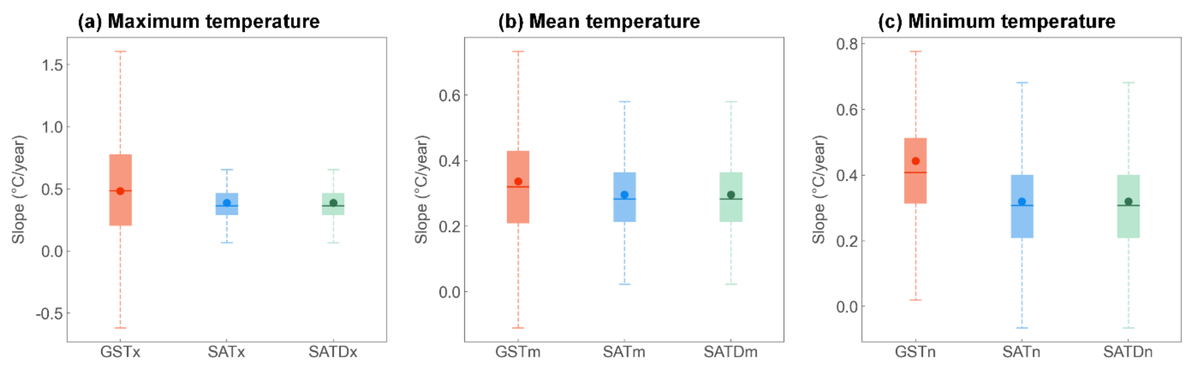
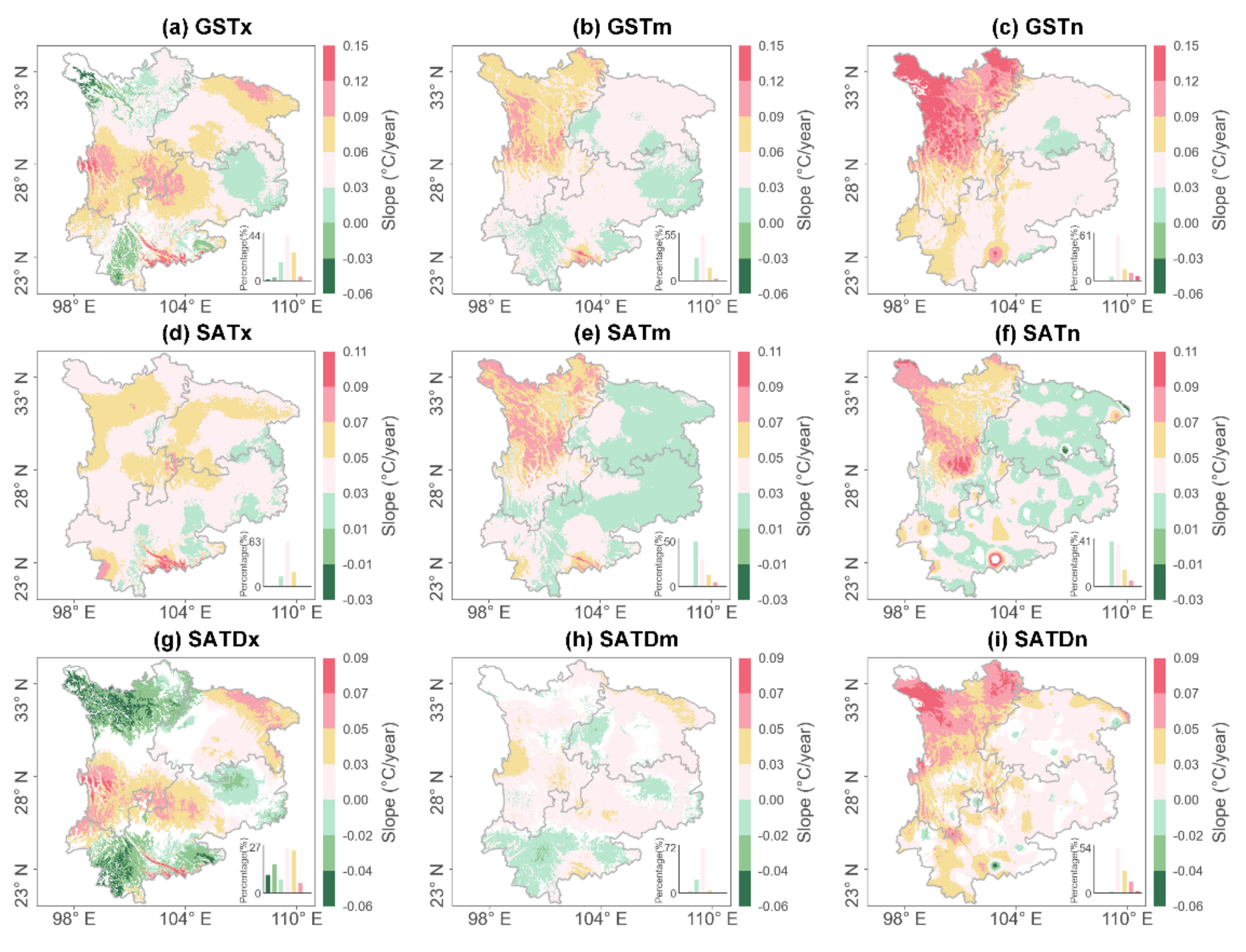
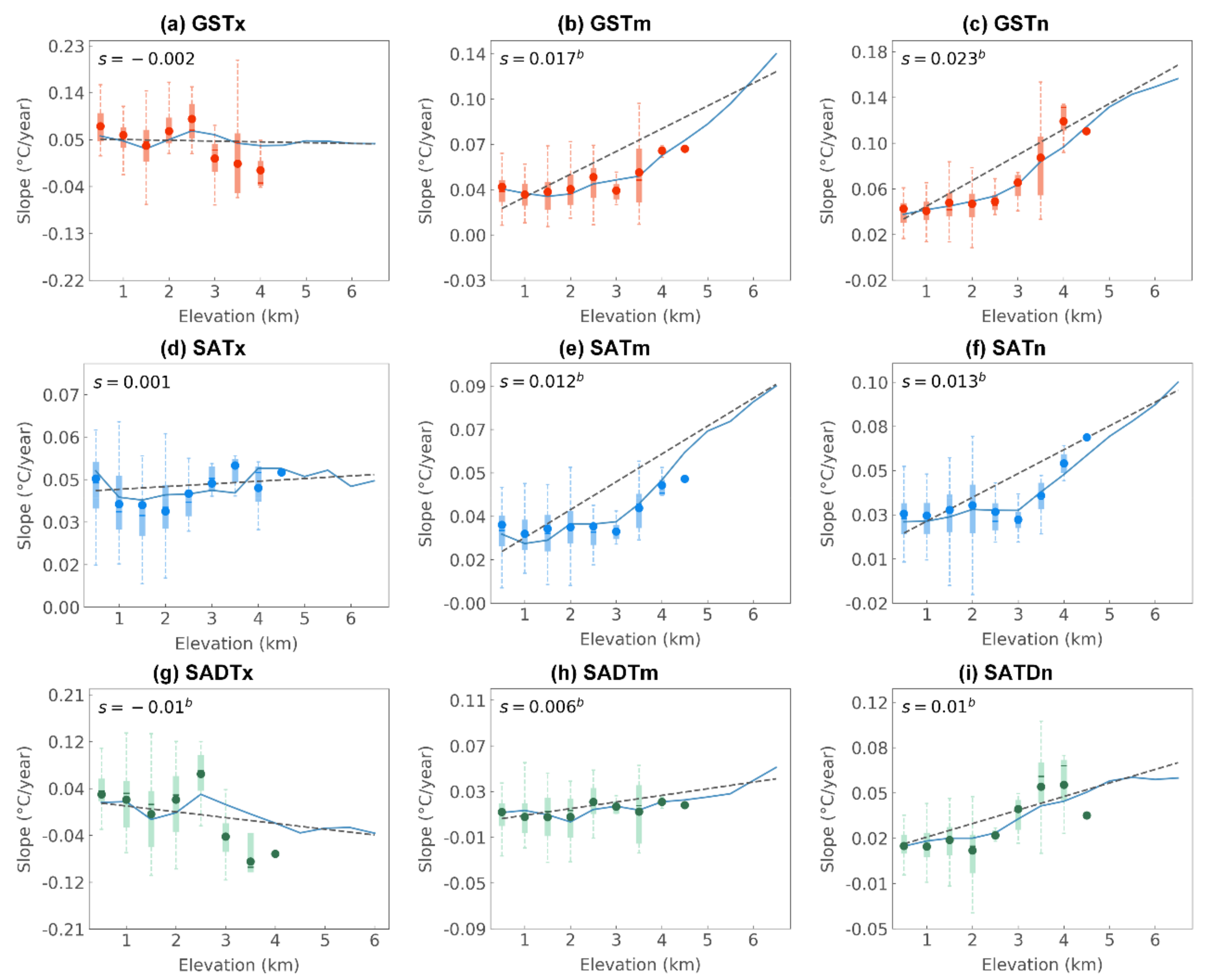
  • Spatially, on annual and seasonal timescales, the variation rate of GSTm and GSTn is consistent with that of SATm and SATn, whereas the variation rate of GSTx is the opposite to that of SATm in high-elevation regions (mainly northern HDM) in SWC. Furthermore, the center of warming of the annual and seasonal GST-, SAT-, and SATD-related indexes is found in the hot dry valley of the Red River (except for SATDx in winter). The variation rate of the annual averaged GSTx and SATDx is downward with elevation, while that of the annual averaged GST, SAT, and SATD is upward with elevation. The elevation variation gradient of the annual averaged GST and SAT amplifies the annual averaged SATD, particularly in HDM.
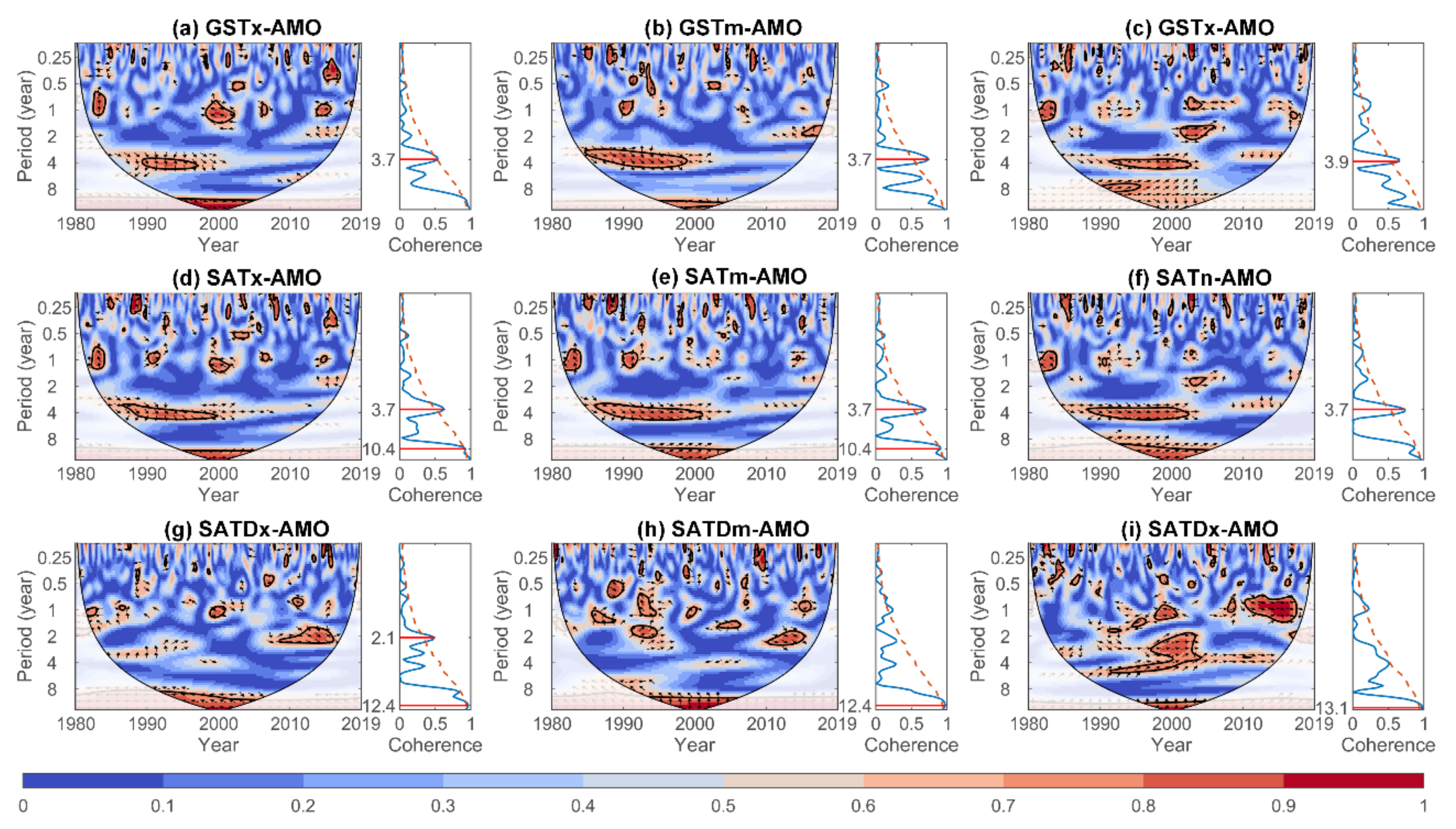
  • The AMO is the large-scale circulation factor with most influence on the anomaly of the monthly averaged GST- and SAT-related indexes on the timescale of 3.7–3.9 years, with a phase difference of +11–75°, indicating that the AMO lags the anomaly of the monthly GST- and SAT-related indexes by 2–9 months in SWC. Meanwhile, the PDO and the NAO lead the anomaly of the monthly averaged SATD-related indexes by 2–5 years (with phase difference −57° to −167°) on the timescale of 12 years, and the most influential large-scale factor in the three subareas exhibits spatial heterogeneity.

Supplementary Materials

The following supporting information can be downloaded at: https://www.mdpi.com/article/10.3390/atmos13071031/s1, Figure S1: Box-and-whisker plots of trends in seasonal averaged GST-, SAT-, and SATD-related indexes in Southwest China (1980–2019). Figures S2–S5: Similar to Figure 6, but for seasonal timescale. Figures S6–S8: Similar to Figure 8, but for subareas. Tables S1 and S2: Variation rate and climate jump of annual/seasonal averaged GST, SAT and SATD related indexes in three subareas. Table S3: Similar to Table 4, but for subareas. Tables S4 and S5: Similar to Table 5 and Table 6, but for subareas. Table S6: Similar to Table 7, but for subareas. Tables S7 and S8: The PASC of bi-wavelet and multiwavelet transform in subareas.

Author Contributions

Conceptualization, Q.C.; methodology, H.J. and Q.C.; validation, P.W.; formal analysis, H.J.; data curation, H.J.; writing—original draft preparation, H.J. and Q.C.; writing—review and editing, P.W. All authors have read and agreed to the published version of the manuscript.

Funding

This study was supported by the supported by Yunnan Fundamental Research Projects (grant no. 202201AU070064), Yunnan Innovative Research Team (no. 202005AE160017), Strategic Priority Research Program of the Chinese Academy of Sciences (grant no. XDA20100104).

Institutional Review Board Statement

Not applicable.

Informed Consent Statement

Not applicable.

Data Availability Statement

The meteorological observed data have been provided by China Meteorological Data Sharing Service System of National Meteorological Information Center (http://www.nmic.gov.cn/) (accessed on 31 December 2019). The multivariate ENSO index (MEI) is provided by the Earth System Research Laboratory Physical Sciences Division at the National Oceanic and Atmospheric Administration (http://www.esrl.noaa.gov/psd/enso/mei/index.html) (accessed on 31 December 2019). Monthly large-scale data (AMO, NAO, AO, PDO, and PNA) is provided from the NOAA National Climatic Data Center (https://psl.noaa.gov/data/climateindices/) (accessed on 31 December 2019), and elevation data (DEM) from the Geospatial Data Cloud of China (http://www.gscloud.cn/) (accessed on 31 December 2019).

Conflicts of Interest

The authors declare no conflict of interest.

References

  1. Liu, B.; Henderson, M.; Wang, L.; Shen, X.; Zhou, D.; Chen, X. Climatology and trends of air and soil surface temperatures in the temperate steppe region of North China. Int. J. Climatol. 2017, 37, 1199–1209. [Google Scholar] [CrossRef]
  2. Shi, X.; Chen, J. Trends in the differences between homogenized ground surface temperature and surface air temperature in China during 1961–2016 and its possible causes. Theor. Appl. Climatol. 2021, 144, 41–54. [Google Scholar] [CrossRef]
  3. Zhang, H.; Yuan, N.; Ma, Z.; Huang, Y. Understanding the Soil Temperature Variability at Different Depths: Effects of Surface Air Temperature, Snow Cover, and the Soil Memory. Adv. Atmos. Sci. 2021, 38, 493–503. [Google Scholar] [CrossRef]
  4. Li, N.; Cuo, L.; Zhang, Y. On the freeze–thaw cycles of shallow soil and connections with environmental factors over the Tibetan Plateau. Clim. Dyn. 2021, 57, 3183–3206. [Google Scholar] [CrossRef]
  5. Chudinova, S.M.; Frauenfeld, O.W.; Barry, R.G.; Zhang, T.; Sorokovikov, V.A. Relationship between air and soil temperature trends and periodicities in the permafrost regions of Russia. J. Geophys. Res. Earth Surf. 2006, 111, F02008. [Google Scholar] [CrossRef] [Green Version]
  6. Qian, B.; Gregorich, E.G.; Gameda, S.; Hopkins, D.W.; Wang, X.L. Observed soil temperature trends associated with climate change in Canada. J. Geophys. Res. Atmos. 2011, 116, D02106. [Google Scholar] [CrossRef]
  7. Hu, G.; Zhao, L.; Li, R.; Wu, X.; Wu, T.; Xie, C.; Zhu, X.; Su, Y. Variations in soil temperature from 1980 to 2015 in permafrost regions on the Qinghai-Tibetan Plateau based on observed and reanalysis products. Geoderma 2019, 337, 893–905. [Google Scholar] [CrossRef]
  8. Wang, X.; Chen, R.; Han, C.; Yang, Y.; Liu, J.; Liu, Z.; Guo, S.; Song, Y. Soil temperature change and its regional differences under different vegetation regions across China. Int. J. Climatol. 2021, 41, E2310–E2320. [Google Scholar] [CrossRef]
  9. Wang, X.; Chen, R.; Han, C.; Yang, Y.; Liu, J.; Liu, Z.; Guo, S.; Song, Y. Response of shallow soil temperature to climate change on the Qinghai–Tibetan Plateau. Int. J. Climatol. 2021, 41, 1–16. [Google Scholar] [CrossRef]
  10. Qin, Y.; Liu, W.; Guo, Z.; Xue, S. Spatial and temporal variations in soil temperatures over the Qinghai–Tibet Plateau from 1980 to 2017 based on reanalysis products. Theor. Appl. Climatol. 2020, 140, 1055–1069. [Google Scholar] [CrossRef]
  11. Jiang, L.; Li, N.; Fu, Z.; Zhang, J. Long-range correlation behaviors for the 0-cm average ground surface temperature and average air temperature over China. Theor. Appl. Climatol. 2015, 119, 25–31. [Google Scholar] [CrossRef]
  12. Luo, D.; Jin, H.; Marchenko, S.S.; Romanovsky, V.E. Difference between near-surface air, land surface and ground surface temperatures and their influences on the frozen ground on the Qinghai-Tibet Plateau. Geoderma 2018, 312, 74–85. [Google Scholar] [CrossRef]
  13. Luo, D.; Liu, L.; Jin, H.; Wang, X.; Chen, F. Characteristics of ground surface temperature at Chalaping in the Source Area of the Yellow River, northeastern Tibetan Plateau. Agric. For. Meteorol. 2020, 281, 107819. [Google Scholar] [CrossRef]
  14. Zhang, W.; Li, S.; Wu, T.; Pang, Q. Changes and spatial patterns of the differences between ground and air temperature over the Qinghai-Xizang Plateau. J. Geogr. Sci. 2007, 17, 20–32. [Google Scholar] [CrossRef]
  15. Garratt, J.R. The atmospheric boundary layer. Earth-Sci. Rev. 1994, 37, 89–134. [Google Scholar] [CrossRef]
  16. Liu, Y.; Wu, G.; Hong, J.; Dong, B.; Duan, A.; Bao, Q.; Zhou, L. Revisiting Asian monsoon formation and change associated with Tibetan Plateau forcing: II. Change. Clim. Dyn. 2012, 39, 1183–1195. [Google Scholar] [CrossRef]
  17. Xin, G.; Yan-Mei, Z.; Da-Wei, H. Temporal and Spatial Characteristics of Soil-Air Temperature Difference (TsTa) in Southeast Guizhou Last 50 Years. Chin. J. Agrometeorol. 2012, 33, 71. [Google Scholar]
  18. Yang, Z.; Gao, J.; Zhou, C.; Shi, P.; Zhao, L.; Shen, W.; Ouyang, H. Spatio-temporal changes of NDVI and its relation with climatic variables in the source regions of the Yangtze and Yellow rivers. J. Geogr. Sci. 2011, 21, 979–993. [Google Scholar] [CrossRef]
  19. Wang, Y.; Chen, W.; Zhang, J.; Nath, D. Relationship between soil temperature in May over Northwest China and the East Asian summer monsoon precipitation. Acta Meteorol. Sin. 2013, 27, 716–724. [Google Scholar] [CrossRef]
  20. Yao-Ming, L.; Deliang, C.; Qiu-Feng, L. The spatiotemporal characteristics and long-term trends of surface-air temperatures difference in China. Adv. Clim. Chang. Res. 2019, 15, 374. [Google Scholar]
  21. Li, J.; Thompson, D.W. Widespread changes in surface temperature persistence under climate change. Nature 2021, 599, 425–430. [Google Scholar] [CrossRef] [PubMed]
  22. He, Y.; Wang, K. Contrast patterns and trends of lapse rates calculated from near-surface air and land surface temperatures in China from 1961 to 2014. Sci. Bull. 2020, 65, 1217–1224. [Google Scholar] [CrossRef]
  23. Wang, J.; Pan, Z.; Han, G.; Cheng, L.; Dong, Z.; Zhang, J.; Pan, Y.; Huang, L.; Zhao, H.; Fan, D. Variation in ground temperature at a depth of 0 cm and the relationship with air temperature in China from 1961 to 2010. Resour. Sci. 2016, 38, 1733–1741. [Google Scholar]
  24. Zhu, F.; Cuo, L.; Zhang, Y.; Luo, J.-J.; Lettenmaier, D.P.; Lin, Y.; Liu, Z. Spatiotemporal variations of annual shallow soil temperature on the Tibetan Plateau during 1983–2013. Clim. Dyn. 2018, 51, 2209–2227. [Google Scholar] [CrossRef]
  25. Fang, X.; Luo, S.; Lyu, S. Observed soil temperature trends associated with climate change in the Tibetan Plateau, 1960–2014. Theor. Appl. Climatol. 2019, 135, 169–181. [Google Scholar] [CrossRef] [Green Version]
  26. Elevation-dependent warming in mountain regions of the world. Nat. Clim. Chang. 2015, 5, 424–430. [CrossRef] [Green Version]
  27. Palazzi, E.; Mortarini, L.; Terzago, S.; Von Hardenberg, J. Elevation-dependent warming in global climate model simulations at high spatial resolution. Clim. Dyn. 2019, 52, 2685–2702. [Google Scholar] [CrossRef] [Green Version]
  28. Rangwala, I.; Miller, J.R. Climate change in mountains: A review of elevation-dependent warming and its possible causes. Clim. Chang. 2012, 114, 527–547. [Google Scholar] [CrossRef]
  29. Shrestha, A.B.; Wake, C.P.; Mayewski, P.A.; Dibb, J.E. Maximum temperature trends in the Himalaya and its vicinity: An analysis based on temperature records from Nepal for the period 1971–94. J. Clim. 1999, 12, 2775–2786. [Google Scholar] [CrossRef] [Green Version]
  30. Thakuri, S.; Dahal, S.; Shrestha, D.; Guyennon, N.; Romano, E.; Colombo, N.; Salerno, F. Elevation-dependent warming of maximum air temperature in Nepal during 1976–2015. Atmos. Res. 2019, 228, 261–269. [Google Scholar] [CrossRef]
  31. Wang, Q.; Fan, X.; Wang, M. Recent warming amplification over high elevation regions across the globe. Clim. Dyn. 2014, 43, 87–101. [Google Scholar] [CrossRef] [Green Version]
  32. Yang, Y.; Wu, Z.; He, H.; Du, H.; Wang, L.; Guo, X.; Zhao, W. Differences of the changes in soil temperature of cold and mid-temperate zones, Northeast China. Theor. Appl. Climatol. 2018, 134, 633–643. [Google Scholar] [CrossRef]
  33. WANG, X.; WANG, S.; JI, C.; PENG, D.; GUO, Y.; ZHENG, X.; Xinjiang, A.B. Spatial-temporal characteristics and mutation analysis of ground temperature in Xingjiang from 1961 to 2015. J. Arid Land Resour. Environ. 2018, 4, 165–169. [Google Scholar]
  34. Zhang, Y.; Sherstiukov, A.B.; Qian, B.; Kokelj, S.V.; Lantz, T.C. Impacts of snow on soil temperature observed across the circumpolar north. Environ. Res. Lett. 2018, 13, 044012. [Google Scholar] [CrossRef] [Green Version]
  35. Park, H.; Sherstiukov, A.B.; Fedorov, A.N.; Polyakov, I.V.; Walsh, J.E. An observation-based assessment of the influences of air temperature and snow depth on soil temperature in Russia. Environ. Res. Lett. 2014, 9, 064026. [Google Scholar] [CrossRef]
  36. Bartlett, M.G.; Chapman, D.S.; Harris, R.N. Snow effect on North American ground temperatures, 1950–2002. J. Geophys. Res. Earth Surf. 2005, 110, F03008. [Google Scholar] [CrossRef] [Green Version]
  37. Yeşilırmak, E. Soil temperature trends in B üyük M enderes B asin, T urkey. Meteorol. Appl. 2014, 21, 859–866. [Google Scholar] [CrossRef]
  38. Liu, J.; Pu, Z. Does soil moisture have an influence on near-surface temperature? J. Geophys. Res. Atmos. 2019, 124, 6444–6466. [Google Scholar] [CrossRef] [Green Version]
  39. Horton, D.E.; Johnson, N.C.; Singh, D.; Swain, D.L.; Rajaratnam, B.; Diffenbaugh, N.S. Contribution of changes in atmospheric circulation patterns to extreme temperature trends. Nature 2015, 522, 465–469. [Google Scholar] [CrossRef] [Green Version]
  40. Wallace, J.M.; Zhang, Y.; Renwick, J.A. Dynamic contribution to hemispheric mean temperature trends. Science 1995, 270, 780–783. [Google Scholar] [CrossRef]
  41. Tung, K.-K.; Zhou, J. Using data to attribute episodes of warming and cooling in instrumental records. Proc. Natl. Acad. Sci. USA 2013, 110, 2058–2063. [Google Scholar] [CrossRef] [PubMed] [Green Version]
  42. Latif, M.; Martin, T.; Park, W. Southern Ocean sector centennial climate variability and recent decadal trends. J. Clim. 2013, 26, 7767–7782. [Google Scholar] [CrossRef] [Green Version]
  43. Gao, L.; Yan, Z.; Quan, X. Observed and SST-forced multidecadal variability in global land surface air temperature. Clim. Dyn. 2015, 44, 359–369. [Google Scholar] [CrossRef]
  44. Banholzer, S.; Donner, S. The influence of different El Niño types on global average temperature. Geophys. Res. Lett. 2014, 41, 2093–2099. [Google Scholar] [CrossRef]
  45. Zhang, G.; Zeng, G.; Li, C.; Yang, X. Impact of PDO and AMO on interdecadal variability in extreme high temperatures in North China over the most recent 40-year period. Clim. Dyn. 2020, 54, 3003–3020. [Google Scholar] [CrossRef]
  46. Zhen-Feng, M.; Jia, L.; Shun-Qian, Z.; Wen-Xiu, C.; Shu-Qun, Y. Observed climate changes in southwest China during 1961–2010. Adv. Clim. Chang. Res. 2013, 4, 30–40. [Google Scholar] [CrossRef]
  47. Ma, Y.; Guan, Q.; Sun, Y.; Zhang, J.; Yang, L.; Yang, E.; Li, H.; Du, Q. Three-dimensional dynamic characteristics of vegetation and its response to climatic factors in the Qilian Mountains. CATENA 2022, 208, 105694. [Google Scholar] [CrossRef]
  48. Yue, S.; Wang, C. The Mann-Kendall test modified by effective sample size to detect trend in serially correlated hydrological series. Water Resour. Manag. 2004, 18, 201–218. [Google Scholar] [CrossRef]
  49. Bao, W.; Shen, D.; Ni, P.; Zhou, J.; Sun, Y. Proposition and certification of moving mean difference method for detecting abrupt change points. J. Geogr. Sci 2018, 73, 2075–2085. [Google Scholar]
  50. Huang, N.E.; Wu, Z. A review on Hilbert-Huang transform: Method and its applications to geophysical studies. Rev. Geophys. 2008, 46, RG2006. [Google Scholar] [CrossRef] [Green Version]
  51. Wu, Z.; Huang, N.E. Ensemble empirical mode decomposition: A noise-assisted data analysis method. Adv. Adapt. Data Anal. 2009, 1, 1–41. [Google Scholar] [CrossRef]
  52. Qian, C.; Wu, Z.; Fu, C.; Wang, D. On changing El Niño: A view from time-varying annual cycle, interannual variability, and mean state. J. Clim. 2011, 24, 6486–6500. [Google Scholar] [CrossRef]
  53. Grinsted, A.; Moore, J.C.; Jevrejeva, S. Application of the cross wavelet transform and wavelet coherence to geophysical time series. Nonlinear Process. Geophys. 2004, 11, 561–566. [Google Scholar] [CrossRef]
  54. Torrence, C.; Compo, G.P. A practical guide to wavelet analysis. Bull. Am. Meteorol. Soc. 1998, 79, 61–78. [Google Scholar] [CrossRef] [Green Version]
  55. Su, L.; Miao, C.; Duan, Q.; Lei, X.; Li, H. Multiple-wavelet coherence of world’s large rivers with meteorological factors and ocean signals. J. Geophys. Res. Atmos. 2019, 124, 4932–4954. [Google Scholar] [CrossRef]
  56. Hu, W.; Si, B.C. Multiple wavelet coherence for untangling scale-specific and localized multivariate relationships in geosciences. Hydrol. Earth Syst. Sci. 2016, 20, 3183–3191. [Google Scholar] [CrossRef] [Green Version]
  57. Hu, W.; Si, B.C.; Biswas, A.; Chau, H.W. Temporally stable patterns but seasonal dependent controls of soil water content: Evidence from wavelet analyses. Hydrol. Process. 2017, 31, 3697–3707. [Google Scholar] [CrossRef]
  58. Schulte, J.A.; Najjar, R.G.; Li, M. The influence of climate modes on streamflow in the Mid-Atlantic region of the United States. J. Hydrol. Reg. Stud. 2016, 5, 80–99. [Google Scholar] [CrossRef] [Green Version]
  59. Chang, X.; Wang, B.; Yan, Y.; Hao, Y.; Zhang, M. Characterizing effects of monsoons and climate teleconnections on precipitation in China using wavelet coherence and global coherence. Clim. Dyn. 2019, 52, 5213–5228. [Google Scholar] [CrossRef] [Green Version]
  60. Shen, B.; Song, S.; Zhang, L.; Wang, Z.; Ren, C.; Li, Y. Temperature trends in some major countries from the 1980s to 2019. J. Geogr. Sci. 2022, 32, 79–100. [Google Scholar] [CrossRef]
  61. Vose, R.S.; Easterling, D.R.; Gleason, B. Maximum and minimum temperature trends for the globe: An update through 2004. Geophys. Res. Lett. 2005, 32, 364–367. [Google Scholar] [CrossRef] [Green Version]
  62. Zhang, Y.; Chen, W.; Smith, S.L.; Riseborough, D.W.; Cihlar, J. Soil temperature in Canada during the twentieth century: Complex responses to atmospheric climate change. J. Geophys. Res. Atmos. 2005, 110, D03112. [Google Scholar] [CrossRef]
  63. Qin, J.; Yang, K.; Liang, S.; Guo, X. The altitudinal dependence of recent rapid warming over the Tibetan Plateau. Clim. Chang. 2009, 97, 321–327. [Google Scholar] [CrossRef]
  64. Gao, Y.; Chen, F.; Lettenmaier, D.P.; Xu, J.; Xiao, L.; Li, X. Does elevation-dependent warming hold true above 5000 m elevation? Lessons from the Tibetan Plateau. npj Clim. Atmos. Sci. 2018, 1, 1–7. [Google Scholar] [CrossRef]
  65. Guo, D.; Sun, J.; Yang, K.; Pepin, N.; Xu, Y. Revisiting recent elevation-dependent warming on the Tibetan Plateau using satellite-based data sets. J. Geophys. Res. Atmos. 2019, 124, 8511–8521. [Google Scholar] [CrossRef] [Green Version]
  66. Tao, J.; Xu, T.; Dong, J.; Yu, X.; Jiang, Y.; Zhang, Y.; Huang, K.; Zhu, J.; Dong, J.; Xu, Y. Elevation-dependent effects of climate change on vegetation greenness in the high mountains of southwest China during 1982–2013. Int. J. Climatol. 2018, 38, 2029–2038. [Google Scholar] [CrossRef]
  67. Wang, Q.; Fan, X.; Wang, M. Warming amplification with both altitude and latitude in the Tibetan Plateau. Int. J. Climatol. 2022, 42, 3323–3340. [Google Scholar] [CrossRef]
  68. Giorgi, F.; Hurrell, J.W.; Marinucci, M.R.; Beniston, M. Elevation dependency of the surface climate change signal: A model study. J. Clim. 1997, 10, 288–296. [Google Scholar] [CrossRef] [Green Version]
  69. Chen, B.; Chao, W.C.; Liu, X. Enhanced climatic warming in the Tibetan Plateau due to doubling CO2: A model study. Clim. Dyn. 2003, 20, 401–413. [Google Scholar] [CrossRef]
  70. Kuttippurath, J.; Murasingh, S.; Stott, P.; Sarojini, B.B.; Jha, M.K.; Kumar, P.; Nair, P.; Varikoden, H.; Raj, S.; Francis, P. Observed rainfall changes in the past century (1901–2019) over the wettest place on Earth. Environ. Res. Lett. 2021, 16, 024018. [Google Scholar] [CrossRef]
  71. Gu, G.; Adler, R.F.; Huffman, G.J. Long-term changes/trends in surface temperature and precipitation during the satellite era (1979–2012). Clim. Dyn. 2016, 46, 1091–1105. [Google Scholar] [CrossRef]
  72. Kundzewicz, Z.W.; Pińskwar, I.; Koutsoyiannis, D. Variability of global mean annual temperature is significantly influenced by the rhythm of ocean-atmosphere oscillations. Sci. Total Environ. 2020, 747, 141256. [Google Scholar] [CrossRef] [PubMed]
  73. Lüdecke, H.-J.; Cina, R.; Dammschneider, H.-J.; Lüning, S. Decadal and multidecadal natural variability in European temperature. J. Atmos. Sol. -Terr. Phys. 2020, 205, 105294. [Google Scholar] [CrossRef]
  74. Ratna, S.B.; Osborn, T.J.; Joshi, M.; Yang, B.; Wang, J. Identifying teleconnections and multidecadal variability of East Asian surface temperature during the last millennium in CMIP5 simulations. Clim. Past 2019, 15, 1825–1844. [Google Scholar] [CrossRef] [Green Version]
  75. Shi, J.; Cui, L.; Ma, Y.; Du, H.; Wen, K. Trends in temperature extremes and their association with circulation patterns in China during 1961–2015. Atmos. Res. 2018, 212, 259–272. [Google Scholar] [CrossRef]
  76. Wang, Y.; Li, S.; Luo, D. Seasonal response of Asian monsoonal climate to the Atlantic Multidecadal Oscillation. J. Geophys. Res. Atmos. 2009, 114, D02112. [Google Scholar] [CrossRef]
  77. Ding, Y.; Liu, Y.; Liang, S.; Ma, X.; Zhang, Y.; Si, D.; Liang, P.; Song, Y.; Zhang, J. Interdecadal variability of the East Asian winter monsoon and its possible links to global climate change. J. Meteorol. Res. 2014, 28, 693–713. [Google Scholar] [CrossRef]
  78. Li, S.; Bates, G.T. Influence of the Atlantic multidecadal oscillation on the winter climate of East China. Adv. Atmos. Sci. 2007, 24, 126–135. [Google Scholar] [CrossRef]
  79. Wang, J.; Yang, B.; Ljungqvist, F.C.; Zhao, Y. The relationship between the Atlantic Multidecadal Oscillation and temperature variability in China during the last millennium. J. Quat. Sci. 2013, 28, 653–658. [Google Scholar] [CrossRef]
  80. Dong, B.; Sutton, R.T.; Scaife, A.A. Multidecadal modulation of El Niño–Southern Oscillation (ENSO) variance by Atlantic Ocean sea surface temperatures. Geophys. Res. Lett. 2006, 33, L08705. [Google Scholar] [CrossRef]
  81. Zhang, R.; Delworth, T.L. Impact of the Atlantic multidecadal oscillation on North Pacific climate variability. Geophys. Res. Lett. 2007, 34, L23708. [Google Scholar] [CrossRef] [Green Version]
  82. Zhu, L.; Cooper, D.J.; Han, S.; Yang, J.; Zhang, Y.; Li, Z.; Zhao, H.; Wang, X. Influence of the atlantic multidecadal oscillation on drought in northern Daxing’an Mountains, Northeast China. Catena 2021, 198, 105017. [Google Scholar] [CrossRef]
  83. Cheng, Q.; Zhong, F.; Wang, P. Potential linkages of extreme climate events with vegetation and large-scale circulation indices in an endorheic river basin in northwest China. Atmos. Res. 2021, 247, 105256. [Google Scholar] [CrossRef]
  84. Schulte, J.; Policelli, F.; Zaitchik, B. A waveform skewness index for measuring time series nonlinearity and its applications to the ENSO–Indian monsoon relationship. Nonlinear Process. Geophys. 2022, 29, 1–15. [Google Scholar] [CrossRef]
  85. Rusu, M.V. The asymmetry of the solar cycle: A result of non-linearity. Adv. Space Res. 2007, 40, 1904–1911. [Google Scholar] [CrossRef]
  86. Timmermann, A. Decadal ENSO amplitude modulations: A nonlinear paradigm. Glob. Planet. Chang. 2003, 37, 135–156. [Google Scholar] [CrossRef]
  87. Gray, S.T.; Graumlich, L.J.; Betancourt, J.L.; Pederson, G.T. A tree-ring based reconstruction of the Atlantic Multidecadal Oscillation since 1567 AD. Geophys. Res. Lett. 2004, 31, L12205. [Google Scholar] [CrossRef]
Figure 1. Distribution of meteorological stations, DEM and subarea division in Southwest China.
Atmosphere 13 01031 g001
Figure 2. Number of observations and pixels in each elevation bin in Southwest China. The blue histogram denotes the number of observations, and the orange line denotes the number of pixels.
Atmosphere 13 01031 g002
Figure 3. Annual averaged timeseries of (ac) GST-, (df) SAT-, and (gi) SATD-related indexes from 1980 to 2019 in Southwest China (a denotes significant at 0.05 level and b denotes significant at 0.01 level. Red dots denote climate jump. Slope denotes variation rate from 1980 to 2019).
Atmosphere 13 01031 g003
Figure 4. Decompositions of monthly averaged (ac) GST-, (df) SAT-, and (gi) SATD-related indexes from 1980 to 2019 into six timescales intrinsic mode function (IMF1–6) using the EEMD.
Atmosphere 13 01031 g004
Figure 5. Box-and-whisker plots of trends in annual averaged GST-, SAT-, and SATD-related indexes from 1980–2019 in Southwest China (a) maximum temperature, (b) mean temperature, (c) minimum temperature (horizontal line represents median, and circle represents average).
Atmosphere 13 01031 g005
Figure 6. Significant variation rate of annual averaged (ac) GST-, (df) SAT-, and (gi) SATD-related indexes for each pixel from 1980 to 2019 in Southwest China. (Significance test by MMK trend method at the 0.05 confidence level). The different colors represent the variation rate and the histograms represent the significant (p ≤ 0.05) percentage of the classified pixel.
Atmosphere 13 01031 g006
Figure 7. Variation rate of annual averaged (ac) GST-, (df) SAT-, and (gi) SATD-related indexes at each elevation bin in Southwest China from 1980 to 2019 (Box-and-whisker, where horizontal line and circle in box-and-whisker denote median and average, respectively, represents variation rate of observed meteorological stations at each elevation bin. Blue folded line represents mean variation rate of interpolated raster at each elevation bin. s denotes slope between annual variation rate of each index with elevation).
Atmosphere 13 01031 g007
Figure 8. Wavelet transform and global coherence of anomaly of the monthly averaged (ac) GST-, (df) SAT-, and (gi) SATD-related indexes with the highest PASC large-scale index from 1980 to 2019 in Southwest China (Red dotted line in global coherence represents significant at 0.05 level).
Atmosphere 13 01031 g008
Table 1. The indexes of the ground soil temperature, surface air temperature and differences between ground soil and air temperature.
ClassificationDefinitionAbbreviation
Surface air temperatureThe maximum air temperature at 2 mSATx
mean air temperature at 2 mSATm
The minimum air temperature at 2 mSATn
Ground soil temperatureThe maximum soil temperature at 0 mGSTx
mean soil temperature at 0 mGSTm
The minimum soil temperature at 0 mGSTn
The difference between ground soil and air temperatureSoil–air maximum temperature differencesSATDx
Soil–air mean temperature differencesSATDm
Soil–air minimum temperature differencesSATDn
Table 2. The interpolation statistics of multiyear averaged GST- and SAT-related indexes.
Optimal Ensemble ModelEnsemble Weights (%)R2 EnsembleR2 Final
GSTxv10.8700.859
GSTmbmv28.7/23.4/47.80.9190.777
GSTnbgmv40/22.8/29.2/80.9680.978
SATxbmv15.5/16.9/67.60.9020.953
SATmbgmv18.7/9/12/60.20.9250.951
SATngmv24.5/52.1/23.40.9290.996
Note, b—boosted regression tree, g—generalized additive model, m—multivariate adaptive regression spline, v—support vector machines. The ensemble weight is the percentage contribution of each algorithm to the ensemble model.
Table 3. Variation rate and climate jump of regional seasonal averaged GST-, SAT-, and SATD-related indexes in Southwest China during 1980–2019.
SpringSummerAutumnWinter
Variation rate (°C/year)GSTx0.065 b0.033 b0.041 b0.042 b
GSTm0.048 b0.021 b0.032 b0.039 b
GSTn0.055 b0.03 b0.042 b0.055 b
SATx0.049 b0.036 b0.035 b0.038 b
SATm0.041 b0.023 b0.027 b0.033 b
SATn0.043 b0.023 b0.031 b0.035 b
SATDx0.019 a−0.0010.008 b0.005 a
SATDm0.008 b-0.003 a0.005 b0.007 b
SATDn0.014 b0.007 b0.013 b0.018 b
Climate jumpGSTx
GSTm
GSTn200320042004
SATx
SATm199620041997
SATn199720042004
SATDx
SATDm 2002
SATDn2003200320032003
Where a denotes significant at 0.05 level and b denotes significant at 0.01 level.
Table 4. Period, variance contribution rate of monthly averaged GST-, SAT-, and SATD-related indexes from 1980 to 2019 in Southwest China.
IMFGSTxGSTmGSTnSATxSATmSATnSATDxSATDmSATDn
Period (year)IMF10.330.240.250.350.550.280.440.250.26
IMF20.980.440.980.980.980.980.980.980.67
IMF31.6711.331.671.91.541.741.381.08
IMF44.051.393.444.064.064.053.933.782.54
IMF58.874.115.679.588.928.129.077.835.09
IMF614.8510.1414.0614.4517.313.9417.3723.4113.18
Variance contribution rate (%)IMF19.2850.347.1112.8518.925.9518.167.0925.59
IMF290.2619.0390.0686.7380.893.2881.5488.360.51
IMF30.228.732.310.210.120.40.161.3911.22
IMF40.187.450.350.150.070.280.090.591.47
IMF50.037.530.080.040.050.060.040.840.65
IMF60.034.570.060.010.020.020.011.160.26
Table 5. Percentage of significant (p ≤ 0.05) increasing/decreasing stations of annual and seasonal averaged GST-, SAT-, and SATD-related indexes in Southwest China from 1980 to 2019.
AnnualSpringSummerAutumnWinter
GSTx69.29/8.4269.02/8.749.18/16.8559.51/8.770.11/6.79
GSTm90.76/1.6390.76/2.9962.77/9.2487.23/1.3691.58/0.82
GSTn97.28/0.2797.28/0.2791.85/1.0993.21/1.0996.74/0.54
SATx96.74/0.8293.75/0.092.93/1.0991.03/0.8292.39/1.09
SATm95.65/0.8294.84/0.087.77/1.3691.85/0.8291.85/1.09
SATn94.84/1.3695.38/0.5490.22/1.993.21/1.6391.58/1.09
SATDx39.95/20.6539.13/19.8430.16/30.4339.4/20.9242.66/21.74
SATDm43.48/23.6443.48/18.7526.63/37.544.57/19.0255.98/16.03
SATDn55.43/12.7758.15/13.3252.17/19.8457.34/12.2360.33/9.78
Table 6. Percentage of significant (p ≤ 0.05) increasing/decreasing pixels of annual and seasonal averaged GST-, SAT-, and SATD-related indexes in Southwest China from 1980 to 2019.
AnnualSpringSummerAutumnWinter
GSTx81.4/3.9677.24/4.4952.88/0.0359.47/0.9653.82/10.56
GSTm99.02/0.0694.56/0.064.62/1.0492.88/0.089.62/0.0
GSTn100.0/0.0100.0/0.0100.0/0.0100.0/0.0100.0/0.0
SATx100.0/0.088.67/0.0798.48/0.082.13/2.3696.61/0.0
SATm99.86/0.096.79/0.0589.62/0.073.33/5.9273.26/0.01
SATn95.55/0.1894.02/0.1499.88/0.093.52/0.088.16/0.52
SATDx37.31/27.0352.0/11.4923.45/10.6424.28/13.215.15/53.49
SATDm50.75/13.9230.08/8.2310.88/42.1883.93/0.7865.55/4.48
SATDn78.78/1.4456.25/10.0676.7/1.2481.07/0.2377.39/1.09
Table 7. The slope (°C/(year·km)) of variation rate of seasonal averaged GST-, SAT-, and SATD-related indexes from 1980 to 2019 with elevation from 64 to 6304 m in Southwest China.
SpringSummerAutumnWinter
GSTx−0.008 b−0.007 b−0.001−0.003
GSTm0.003 b0.004 b−0.0010.005 b
GSTn0.003 b0.008 b0.026 b0.029 b
SATx−0.005 b0.001−0.0020.008 b
SATm−0.005 b0.005 b−0.024 b−0.003
SATn0.0080.006 b−0.0010.005 b
SATDx−0.001−0.0040.008 b−0.012 b
SATDm0.01 b−0.005 a0.02 b0.006 b
SATDn0.0040.003 b0.028 b0.031 b
Where a denotes significant at 0.05 level and b denotes significant at 0.01 level.
Table 8. Percentage area of significant (p ≤ 0.05) coherence in bi-wavelet transform coherence between the anomaly of the monthly averaged GST-, SAT-, and SATD-related indexes and large-scale indexes in from 1980 to 2019 in Southwest China.
GSTmGSTxGSTnSATmSATxSATnSATDxSATDnSATDm
AMO12.0311.615.1812.3110.912.115.257.626.02
AO5.816.553.974.774.74.227.198.958.54
MEI3.854.62.574.193.813.899.348.2812.37
NAO3.884.322.813.463.772.5211.2213.713.76
PDO4.343.864.823.514.363.5112.018.439.27
PNA3.384.763.775.245.064.649.385.671.58
Entries in bold indicate the large-scale index with the highest PASC.
Table 9. Main results obtained by WTC for strongest relationships between monthly abnormal averaged GST-, SAT- and SATD-related indexes and the most influential large-scale index in Southwest China from 1980 to 2019.
Interannual ScaleInterdecade Scale
The Most Influential Large-Scale FactorCoherence Period (Year)YearsPhase Difference (°)Leads/Lags (Month)Coherence Period (Year)YearsPhase Difference (°)Leads/Lags (Year)
GSTxAMO3.71989–199375.9+9.3
GSTmAMO3.71988–199747+5.8
GSTnAMO3.91991–200111.1+1.4
SATxAMO3.71988–199259.2+7.310.41980–198511.3+0.32
SATmAMO3.71986–199740.6+510.41980–1997−7.3−0.2
SATnAMO3.71988–200023.6+2.9
SATDxPDO2.12010–201535.3+2.412.41980–2019−161.7−5.5
SATDmNAO 12.41980–2019−86.1−3
SATDnNAO 13.11980–2019−57.8−2.1
+ denotes the phase of monthly averaged GST, SAT and SATD-related indexes anomaly lead phase of large-scale indexes; − denotes the phase of abnormal averaged GST, SAT and SATD-related indexes lag phase of large-scale indexes.
Table 10. Percentage area of significant coherence (PASC) in multi-wavelet transform coherence between the anomaly of the monthly averaged GST-, SAT-, and SATD-related indexes and large-scale indexes from 1980 to 2019 in Southwest China.
Maximum TemperatureMean TemperatureMinimum Temperature
CombinationPASC (%)CombinationPASC (%)CombinationPASC (%)
GSTAMO11.61AMO12.03AMO5.18
AMO+AO12.96AMO+NAO12.60AMO+PDO21.40
AMO+AO+MEI9.93AMO+NAO+PNA12.65AMO+PDO+NAO18.68
AMO+AO+MEI+NAO9.91AMO+NAO+PNA+AO11.69AMO+PDO+NAO+PNA15.23
SATAMO10.90AMO12.31AMO12.11
AMO+AO11.06AMO+NAO12.28AMO+PNA12.32
AMO+AO+NAO9.70AMO+NAO+PNA11.49AMO+PNA+NAO12.33
AMO+AO+NAO+PNA9.81AMO+NAO+PNA+AO10.90AMO+PNA+NAO+PDO12.02
SATDPDO12.01NAO13.76NAO13.70
PDO+PNA17.15NAO+PDO16.67NAO+AMO22.82
PDO+PNA+NAO13.42NAO+PDO+AMO14.67NAO+AMO+MEI14.77
PDO+PNA+NAO+AMO13.51NAO+PDO+AMO+AO14.24NAO+AMO+MEI+AO13.66
Publisher’s Note: MDPI stays neutral with regard to jurisdictional claims in published maps and institutional affiliations.

