Observation of Gravity Wave Vertical Propagation through a Mesospheric Inversion Layer

Abstract

The impact of a mesospheric temperature inversion on the vertical propagation of gravity waves has been investigated using OH airglow images and ground-based Rayleigh lidar measurements carried out in December 2017 at the Haute-Provence Observatory (OHP, France, 44N). These measurements provide complementary information that allows the vertical propagation of gravity waves to be followed. An intense mesospheric inversion layer (MIL) observed near 60 km of altitude with the lidar disappeared in the middle of the night, offering a unique opportunity to evaluate its impact on gravity wave (GW) propagation observed above the inversion with airglow cameras. With these two instruments, a wave with a 150 min period was observed and was also identified in meteorological analyses. The gravity waves’ potential energy vertical profile clearly shows the GW energy lost below the inversion altitude and a large increase of gravity wave energy above the inversion in OH airglow images with waves exhibiting higher frequency. MILs are known to cause instabilities at its top part, and this is probably the reason for the enhanced gravity waves observed above.

1. Introduction

Atmospheric gravity waves (AGW) play significant roles in the dynamics of the atmosphere. Their ability to transport energy from the lower atmosphere to the mesosphere lower thermosphere (MLT) has been widely studied [1,2,3]. Without dissipation, AGW energies increase exponentially with altitude following the scale height of the atmospheric density. Such waves are generated in the troposphere through different processes, including thunderstorm [4], convection, and wind flow over mountains, and they propagate vertically and horizontally [5,6,7,8]. Waves generated in the troposphere propagating up to the thermosphere have been mostly associated with tsunami [9]. In practice, most AGWs are filtered while breaking in the MLT. During their vertical propagation, waves interact with the mean flow through momentum transfer and energy dissipation when waves break [2,10], especially in the mesosphere. These waves contribute significantly to large-scale atmospheric circulation and the 3D dynamic fields of temperature and wind. Potential energy of gravity waves derived with lidar data has shown such energy reduction above 60–70 km altitude [11]. Additionally, these interactions frequently induce MILs that can last for a few days with temperature differences of a few tens of degrees [12].

Wave properties from the troposphere up to the mesosphere cannot be observed with a single instrument. Rayleigh lidar measurements of temperature with high temporal resolutions are commonly used to conduct gravity wave studies in the stratosphere and mesosphere [13,14]. However, in the mesosphere, the signal-to-noise ratio decreases rapidly with altitude and does not allow the calculation of spectral analyses of small scale waves from statistical noise [15]. Although the variance of the backscattered signal can provide global information on wave activity higher up [11], information is still limited to 70 km altitude depending on the lidar capabilities. It is well known that AGW induce airglow fluctuations of the hydroxyl OH Meinel bands layer around 87 km altitude with a half-width of approximately 8 km [16]. These fluctuations can be observed using CCD imagers operating in the near infrared wavelength region [17,18,19] as well as in the short wave infrared (SWIR) band [20,21] using InGaAs imaging systems.

Combined lidar temperature and airglow observations allows the observation of AGWs at different altitudes during their propagation. Several studies have previously used the synergy between these two instruments to study gravity wave events using mesospheric OH airglow image measurements and ground-based lidar data [22,23].

Although gravity waves generate MILs for several days, the wave propagation through this type of structure has not yet been described. It is therefore interesting to better document how the troposphere and thermosphere are coupled and to what extent characteristics of gravity waves propagating from below remain similar in the thermosphere and can provide information about their sources. A strong westerly stratospheric jet can produce a filtering of westerly gravity wave drag, resulting in an enhanced easterly drag in the mesosphere and associated anomalous warming of the upper mesosphere [24,25]. This situation is favorable to MIL formation. The sharp mesospheric wind gradient may be a source of dynamical instabilities and generation of secondary gravity waves [26]. The state of the polar vortex plays a role in the modulation of GW activity and formation of MILs. For instance, the cooling of the lower mesosphere after a sudden stratospheric warming event promotes the propagation of GWs and the formation of MILs in the upper mesospheric polar region [27].

In order to study gravity wave propagation through the atmosphere, a SWIR imaging system to measure the nightglow radiation emitted by OH at an altitude of 87 km was operated next to a routinely operating ground-based Rayleigh lidar that was providing a 2D temperature profile as a function of altitude and time since 1979. During this campaign, a MIL inducing a large temperature disturbance was present around 65 km altitude and disappeared during the continuous instrumental operation around midnight, providing a unique opportunity to study the AGW propagation through a disturbed mesosphere. Such investigations were already simulated by Fritts et al. [28] or Fritts et al. [29] using a numerical model. Observations conducted during this night were analyzed to confirm and document some findings of these theoretical studies.

In this study, we describe the impact of an MIL on AGW propagation by comparing gravity wave activity from 25 to 65 km altitude using Rayleigh lidar and meteorological analyses with OH layer observations at 87 km. Section 2 describes the different datasets used in this study. Section 3 presents the gravity wave analyses, and Section 4 describes the impact of the MIL on the vertical GW propagation. Finally, Section 5 provides discussions and conclusions.

2. Description of the Campaign and the Instruments

The observation campaign was carried out at the OHP in the south of France during the night of 12 to 13 December 2017. The campaign was performed in the frame of the European Atmospheric dynamics Research InfraStructure In Europe (ARISE) framework [30]. This project intends to set up a network of instruments to investigate the atmospheric dynamic and the vertical coupling between ground anomalies up to the lower thermosphere. The infrastructure is composed of a dense network of infrasound instruments that are intend to be assimilated to provide wind constraints, and prototype stations having several collocated instruments including lidars, microwave spectrometers, and radars that provide complementary information about waves at different scales.

The good atmospheric transparency experienced during the night of 12 to 13 December permitted the best optical observations. The presence of a strong mesospheric inversion layer during the first part of the night and its rapid extinction at midnight offered a unique opportunity to study its impact on wave propagation.

2.1. Lidar Measurements

Lidars can provide vertical temperature and density profiles using Rayleigh scattering, as demonstrated by Hauchecorne and Chanin [31]. Observations are based on the backscattering light collected with large ground-based telescopes and generated by pulse lasers emitted vertically from the ground. This technique is now well established [32], and the integration of successive laser shots over several hours allows one to derive temperature from 30 to 80–90 km altitude. Continuous measurements have been performed within the Network for the Detection of Stratospheric Changes (NDSC) during more than 4 decades to monitor temperature changes [33,34].

Such continuous measurements have been performed in the framework of the international Network of the Detection of Atmospheric Composition Changes (NDACC) [35] and in the framework of ARISE [30]. The good vertical resolution and small time integration over periods of several minutes allow for the derivation of time and vertical temperature fluctuations induced by the propagation of gravity waves [15].

However, spectral fluctuations in the mesosphere are constrained and limited to waves with periods around several minutes (typically 10–15 min) with vertical resolution typically 10–100 m to keep a signal-to-noise ratio larger than the wave amplitudes. Figure 1 shows the 2D temperature profile during the night of 12–13 December 2017 above OHP. Detailed spectral wave information cannot be obtained in the mesosphere. To avoid this range limitation due to the smaller signal-to-noise ratio, a new method has been developed to access the potential energy of gravity waves based on the analysis of the 2D variability [11].

2.2. The Airglow Camera

An airglow camera based on a thermoelectrically cooled InGaAs detector (640 × 512 pixels, pitch 25 µm) was used during the observation campaign. The spectral bandwidth of the camera ranges from 0.9 to 1.7 µm. This bandwidth corresponds to the vibrational transitions $\mathsf{\Delta }\nu$ = 2 and 3 of the OH Meinel band system. The integration time used is 400 ms with a frame rate of 0.5 s. Thus, for the entire night, we acquired approximately 50,000 images.

Obviously, such a frame rate is not useful for this study; however, it was chosen initially to investigate the impact of infrasound on OH radiation [20]. A 12.5 mm focal lens was mounted on the camera, leading to a field of view (FOV) of 32 × 27, which allowed us to observe a 111 × 89 km area at the OH layer altitude (∼87 km) for a zenith observation. The instantaneous field of view of 2 mrad led to a spatial resolution of 174 m at the altitude of the OH layer. The camera is radiometrically calibrated in a low light level laboratory at Onera, allowing absolute integrated radiance measurements (in photons/s/m²/sr). After the campaign, the acquired raw images are radiometrically corrected (dark current, dome effect) and unwarped, giving all the information to retrieve wave parameters for ours studies. Figure 2 shows an image acquired during the campaign.

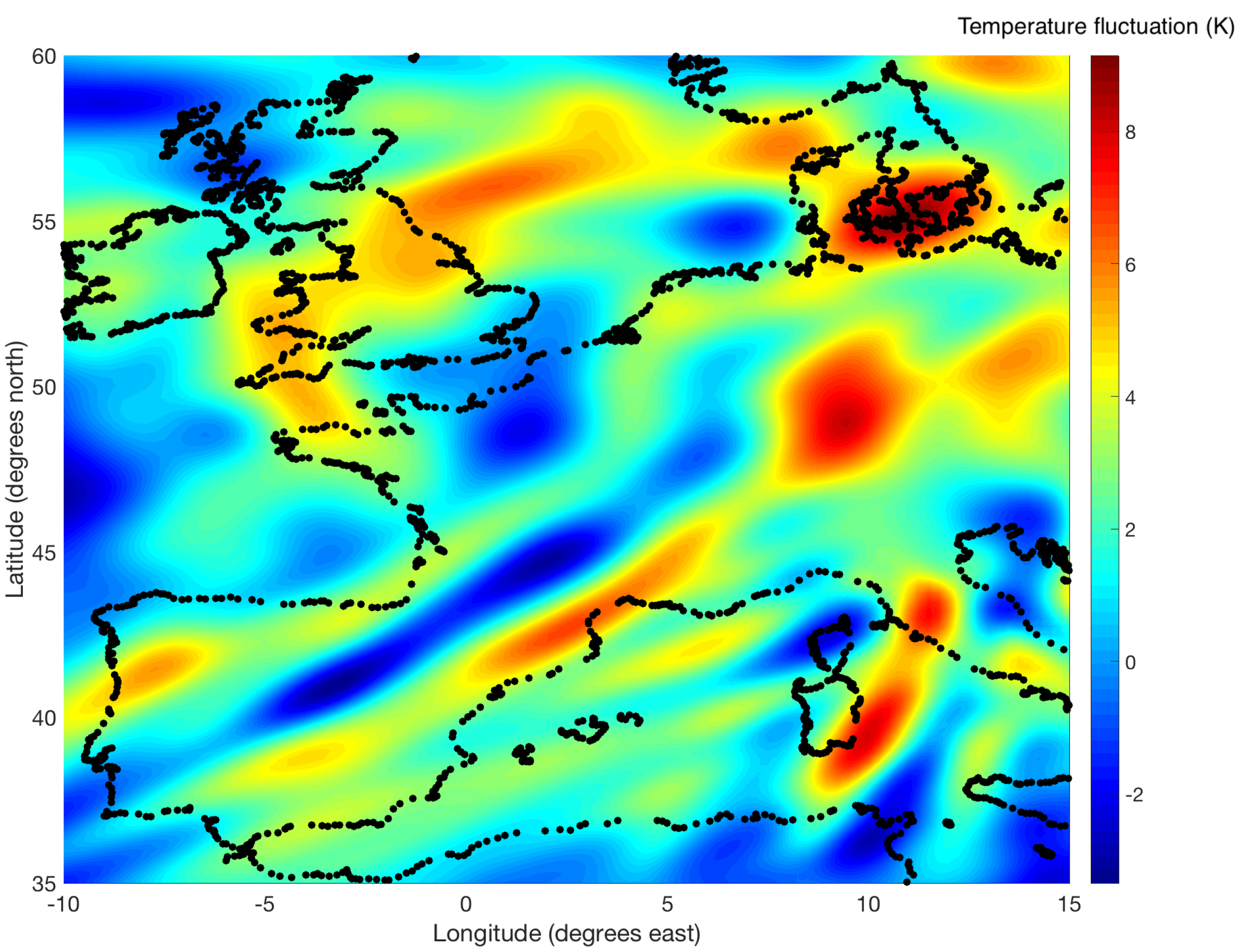
2.3. European Meteorological Analyses (ERA5 Data)

Products extracted from the European meteorological re-analysis include many variables, such as wind speed, temperature, and atmospheric pressure, dedicated to meteorological applications but are also a reference for any atmospheric researches. An important advantage of re-analyses is that they are generally available worldwide and provide a realistic mean atmospheric evolution due to all the global assimilated observations. Over the decades, re-analyses were regularly improved, providing a wider vertical range and greater resolution in time and space.

Within the Copernican Climate Change Service (C3S), the European Centre for Medium-Range Weather Forecasts (ECMWF) is producing the ERA5 re-analysis that, when completed, will provide a detailed record of the global atmosphere, land surface, and ocean waves from 1950 onwards. Unlike its predecessor ERA-Interim, ERA5 has hourly resolution and wind speed data available free of charge at 100 m height and up to the maximum altitude of 79 km, which is important for our study. The horizontal resolution is about 31 km, which is better than ERA-Interim. A clear wave structure (Figure 3) is reported on the observations night, showing that ECMWF is now able to capture gravity waves with long wavelengths.

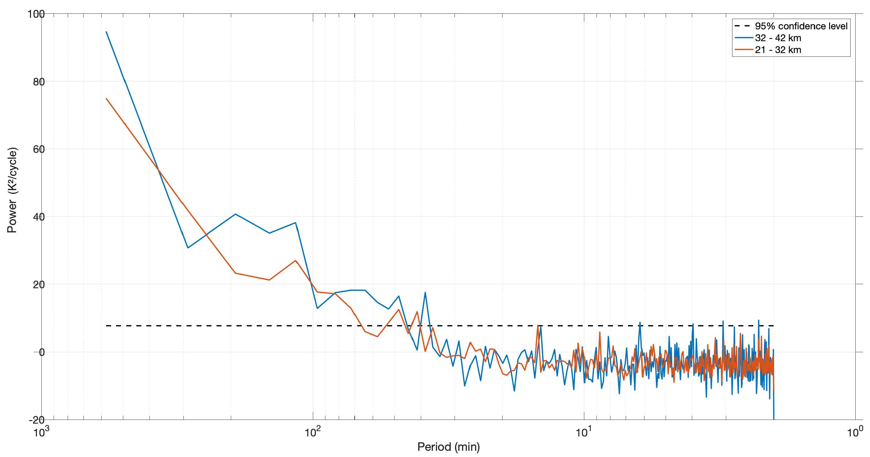
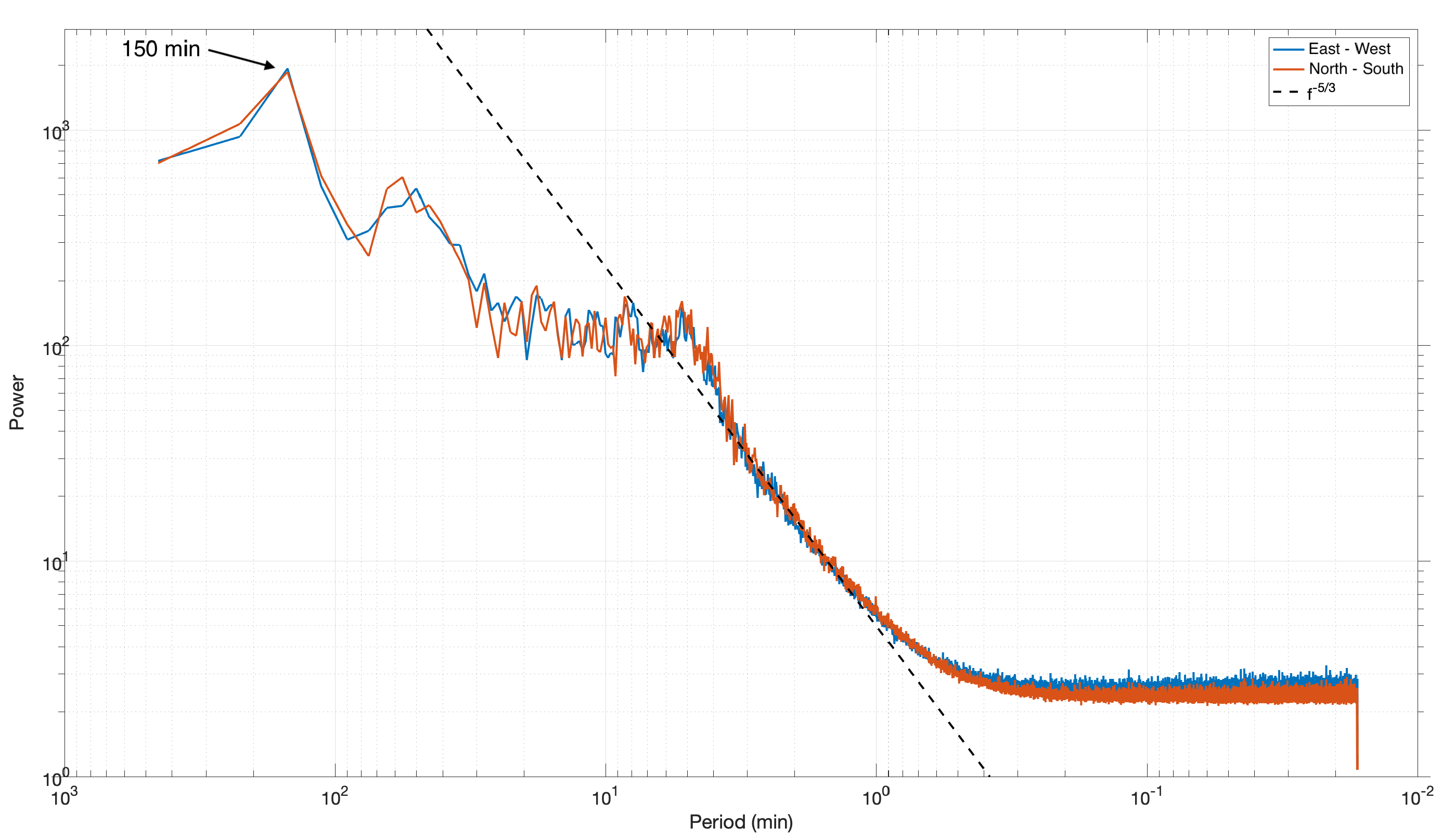
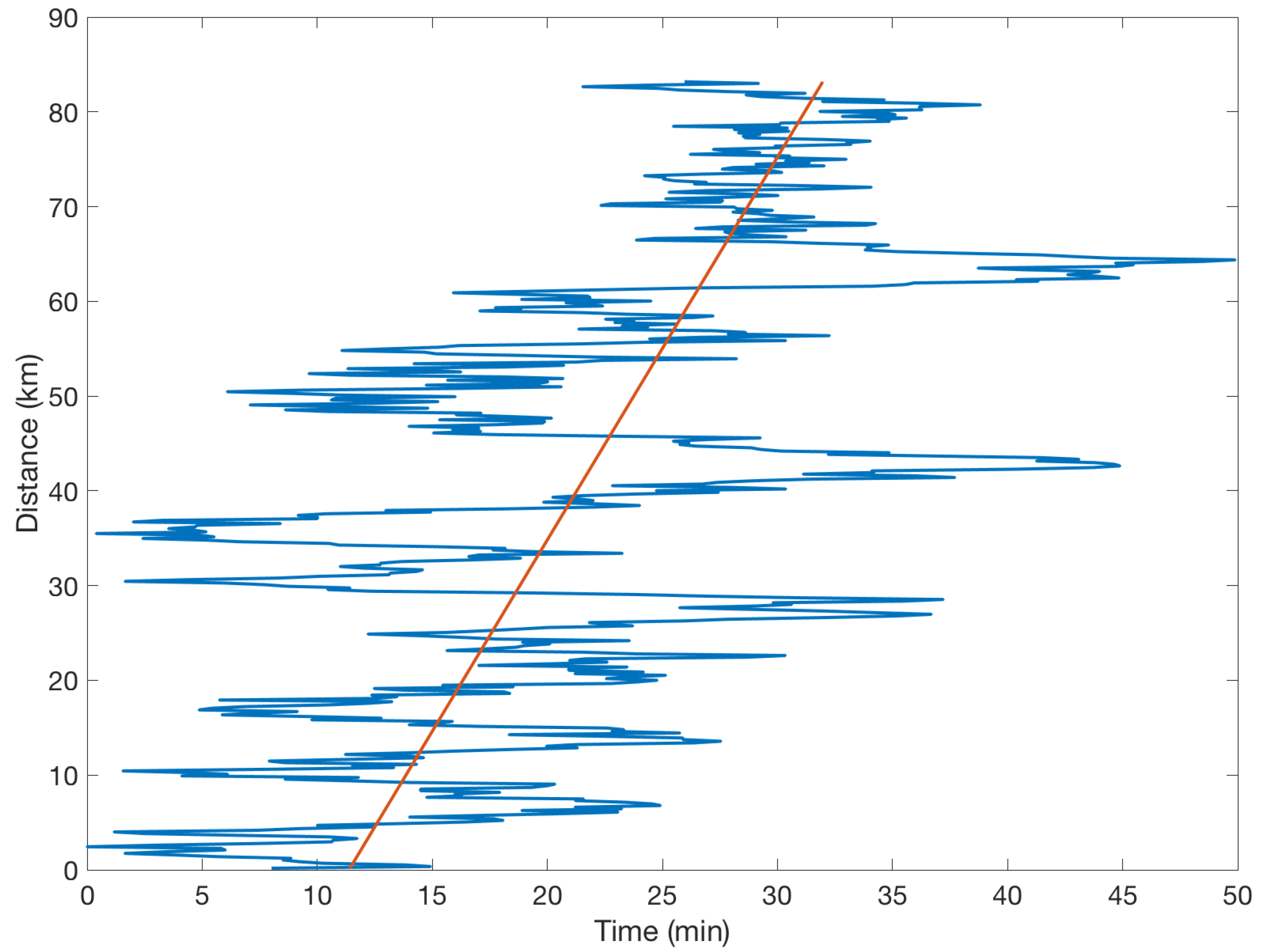
3. Gravity Wave Analyses

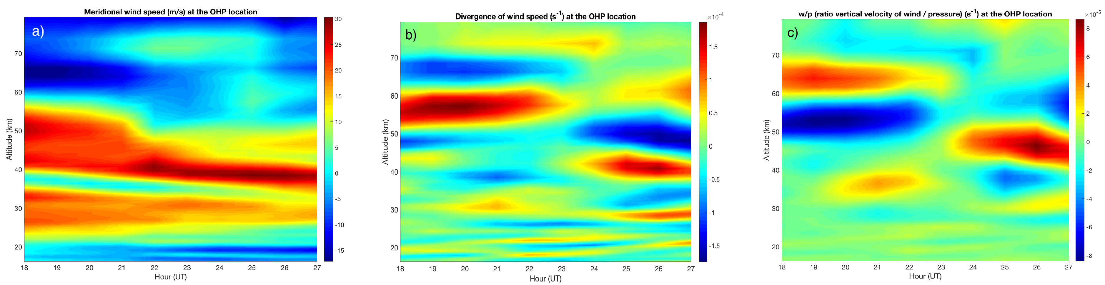
3.1. Vertical Propagation Analysis Using ERA5 Data, Rayleigh Lidar, and OH Airglow Observations

In order to determine the frequency of temperature fluctuations, Fourier transforms are applied on observations to characterize the activity of gravity waves either as a function of time or altitude. Before applying the Fourier transform, the signals are pre-processed. For each temperature perturbation, we remove linear trends and multiply by a Hanning window ($\alpha$ = 0,1) so that the edges are set to zero. Fourier transform is applied to temperature perturbations at each altitude, and spectra are averaged to improve the signal-to-noise ratio.

The mean Fourier spectrum for the temperature lidar data is calculated for two altitude domains, [21–32] and [32–42] km in summing all 10 individual spectra for each time series (Figure 4). These 10 individual spectra are computed from time series for 10 heights within the two height ranges. In order to determine confidence level, noise is calculated by generating a white Gaussian noise for each lidar level with similar standard deviations to the lidar uncertainties. Nevertheless, the noise depends on the level of the lidar signals, which decreases with altitude. Therefore, such Fourier analysis cannot be performed above the stratopause (50 km) because the signal-to-noise ratio is too small to show significant power due to atmospheric waves.

Significant peaks are identified at periods in the intervals 40–90 and 100–300 min. The periods under 10 min are associated with noise. The Brunt–Väisälä frequency is calculated by the following equation:

$$N^2=\frac{g}{T}\left(\frac{dT}{dz}+\mathsf{\Gamma }\right)$$

(1)

where g = 9.81 m.s⁻¹ is the gravitational acceleration, T is the temperature, $\mathsf{\Gamma }$ is the atmospheric lapse rate, and z is the altitude.

Because airglow images cover a 111 × 89 km region at the OH layer altitude, observation of large-scale gravity waves is not possible using only individual images. Therefore, in order to study waves with wavelengths exceeding the field of view of the image, a keogram analysis is performed by considering the central columns of each image (54,000 columns) and placing them side-by-side to form a single image (Figure 5). This analysis can be performed in both directions (with also the central row) generating, respectively, a north–south keogram and an east–west keogram. The result presents the wave field during the night. On the figure, we can observe wave systems with short and quite long periods.

Fourier transform is applied on the north–south keogram in order to analyze the wave frequency content of the night. The data are pre-processed in summing each individual Fourier transform of each row of the keograms in order to determine the low frequencies present throughout the night (Figure 6).

In the Fourier transform of keograms, a peak around the 150 min period is detected. Spectra show that the energy increases until the Brunt–Väisälä period (around 5 min at the OH layer altitude) following the −5/3 power law stabilizes until 20 min and finally increases until 150 min. The increases in energy up to the Brunt–Väisälä period may be due to the creation of turbulence caused by the MIL. The stabilization from the Brunt–Väisälä period up to 30 min is probably due to the trapping of small-scale gravity waves by the MIL, as opposed to the periods after 30 min, where the slope is again positive. This suggests a free propagation of large-scale gravity waves.

The frequency characteristics reported by keograms are observed parameters. To determine the intrinsic frequencies, the following Doppler relation between intrinsic and observed periods is used:

$$\begin{array}{c}\hfill \widehat{\omega }={\omega }_{obs}-ku-lv\end{array}$$

(2)

where $\widehat{\omega }$ is the intrinsic frequency, ${\omega }_{obs}$ is the observed frequency, k and l are, respectively, the zonal and meridional wavenumbers, and u, v are, respectively, the mean zonal and meridional wind speeds at the OH layer altitude.

The local wind speed is estimated with the Horizontal Wind Model (HWM07) [36] to include the tidal component. The HWM07 model has a non-negligible error at high altitude. The main error on the wind speed at these altitudes comes from the tides. We will therefore assume an error of 20 m/s for the meridional and zonal wind speed. This number corresponds to the average tidal range in the upper atmosphere [37,38,39,40,41]. The HWM07 model was used instead of its improved version, namely, HWM14 [42] because we are used to using it and HWM14 was not available. However, we may use it for future studies. To estimate the zonal and meridional wavenumbers for the long periods, keograms were filtered with a third-order bandpass filter between 130 and 170 min to isolate the 150 min period. The temporal evolution of the 150 min wave phase (Figure 7, blue curve) using a sine fit was then estimated.

Once the phase of the wave was calculated, a slope that corresponds to the phase velocity of the wave was measured, and we then calculated the wavelength using the intrinsic period. For the determination of the meridional and zonal wavelengths we used, respectively, the north–south and the east–west keograms. For example, the slope of the linear fit for the east–west keogram is 4.04 ± 0.5 km/min. A meridional wavelength of 605 km and a zonal wavelength of 848 km were determined.

The intrinsic frequency can be deduced from the wavelength estimate using Equation (2). The vertical wavenumber is then calculated using the dispersion relation (3) and the group velocity from Equation (4). These equations are derived from linear gravity wave theory [43].

$$m^2=\frac{K^2\left(N^2-\widehat{{\omega }^2}\right)}{\left(\widehat{{\omega }^2}-f^2\right)}-\frac{1}{4{H^2}_s}$$

(3)

where $H_s$ is the scale height (7 km).

$$\left(c_{gx},c_{gy},c_{gz}\right)=\frac{\left[k\left(N^2-\widehat{{\omega }^2}\right),l\left(N^2-\widehat{{\omega }^2}\right),m\left(\widehat{{\omega }^2}-f^2\right)\right]}{\widehat{\omega }\left(K^2+m^2+\frac{1}{4H^2}\right)}$$

(4)

with $K=\sqrt{k^2+l^2}$ and f is the Coriolis parameter. The computed intrinsic parameters and the corresponding errors are compiled in

Table 1. Intrinsic parameters of the 150 min wave. From left to right: the observed period, the intrinsic period, the zonal wavelength, the meridional wavelength, the horizontal wavelength, the intrinsic horizontal phase speed, the vertical wavelength, the group velocity, and the direction of propagation.

$\mathit{\omega }$ (min)	$\widehat{\mathit{\omega }}$ (min)	${\mathit{\lambda }}_{\mathit{x}}$ (km)	${\mathit{\lambda }}_{\mathit{y}}$ (km)	${\mathit{\lambda }}_{\mathit{h}}$ (km)	${\mathit{V}}_{\mathit{h}}$ (m/s)	${\mathit{\lambda }}_{\mathit{v}}$ (km)	${\mathit{c}}_{\mathit{g}}$ (m/s)	$\mathit{\theta }$ (deg)
150	243 ± 40	605 ± 76	848 ± 224	492 ± 100	33 ± 10	14 ± 5	32 ± 13	135

.

The direction of propagation ($\theta$ in Table 1) was estimated using the inclination of the phases evolution of the wave taken from the two filtered keograms; $\theta$ was measured anticlockwise from the east. It can be observed that the intrinsic period obtained is included in the period band where we observe a significant energy in the lidar Fourier spectrum for the 32–42 km altitude band (Figure 4). It can be concluded that large-scale gravity waves are well transmitted through the MIL.

Wave activity was also extracted from the ERA5 dataset extrapolated for this night over an area centered on France with the following spatial extent: −10 to 15 of longitude and 35 to 60 of latitude. The average temperature was calculated by summing hourly values and subtracting the result from each map to determine the temperature anomalies. The Fourier transform results for each map were averaged in time and altitude to obtain the mean spectrum (Figure 8). In order to increase the resolution of the average spectrum, the maps were centered in a matrix of 1101*1101 zero-filled pixels, and an apodization window was applied to reduce discontinuities.

The horizontal wavenumbers deduced from ERA5 in the altitude domain 26–36 km and 42–48 km are in good agreement with the OH data at 87 km altitude where the wavelengths of the wave were estimated using the keograms (white cross on the figures). If we assume that the lidar and ERA5 data below 87 km altitude observe the same wave, we can therefore conclude that this large-scale wave propagated at least up to 87 km, the altitude of the OH layer, despite the presence of the MIL. These results are consistent with the findings of Fritts et al. [28].

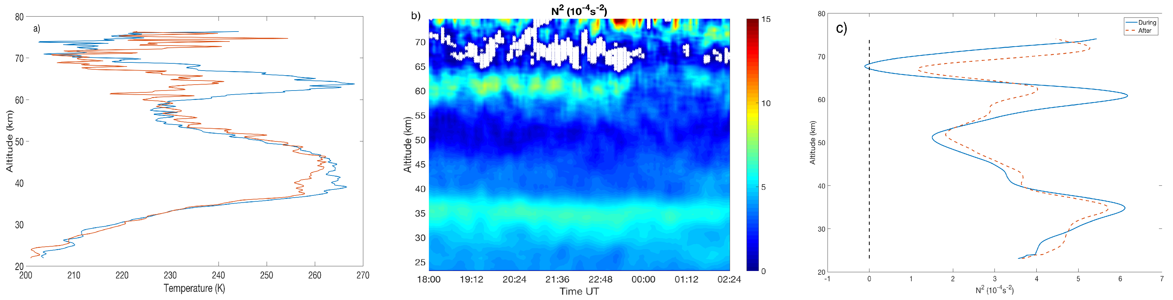
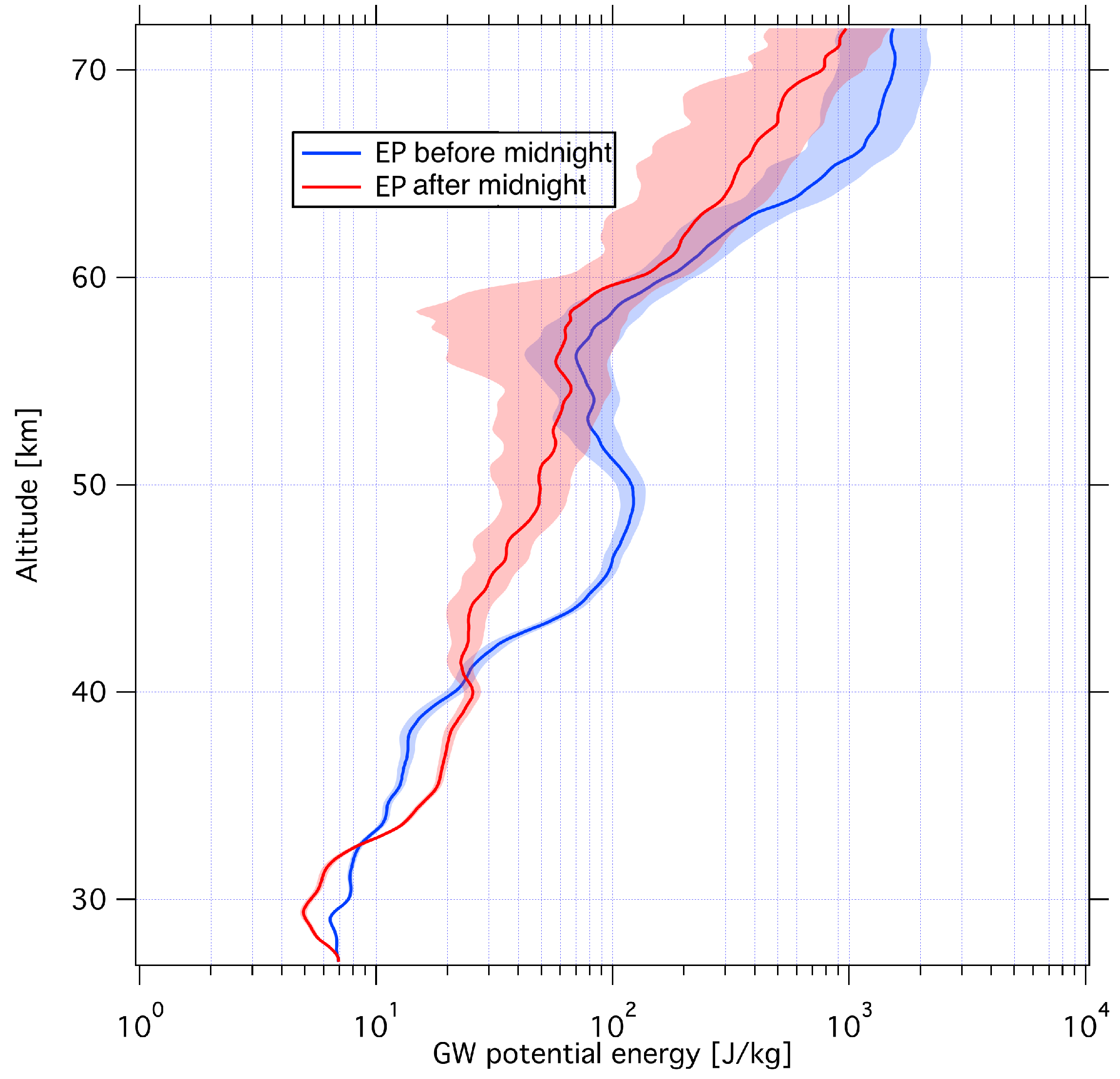
4. Impact of the MIL on the Vertical Gravity Wave Propagation

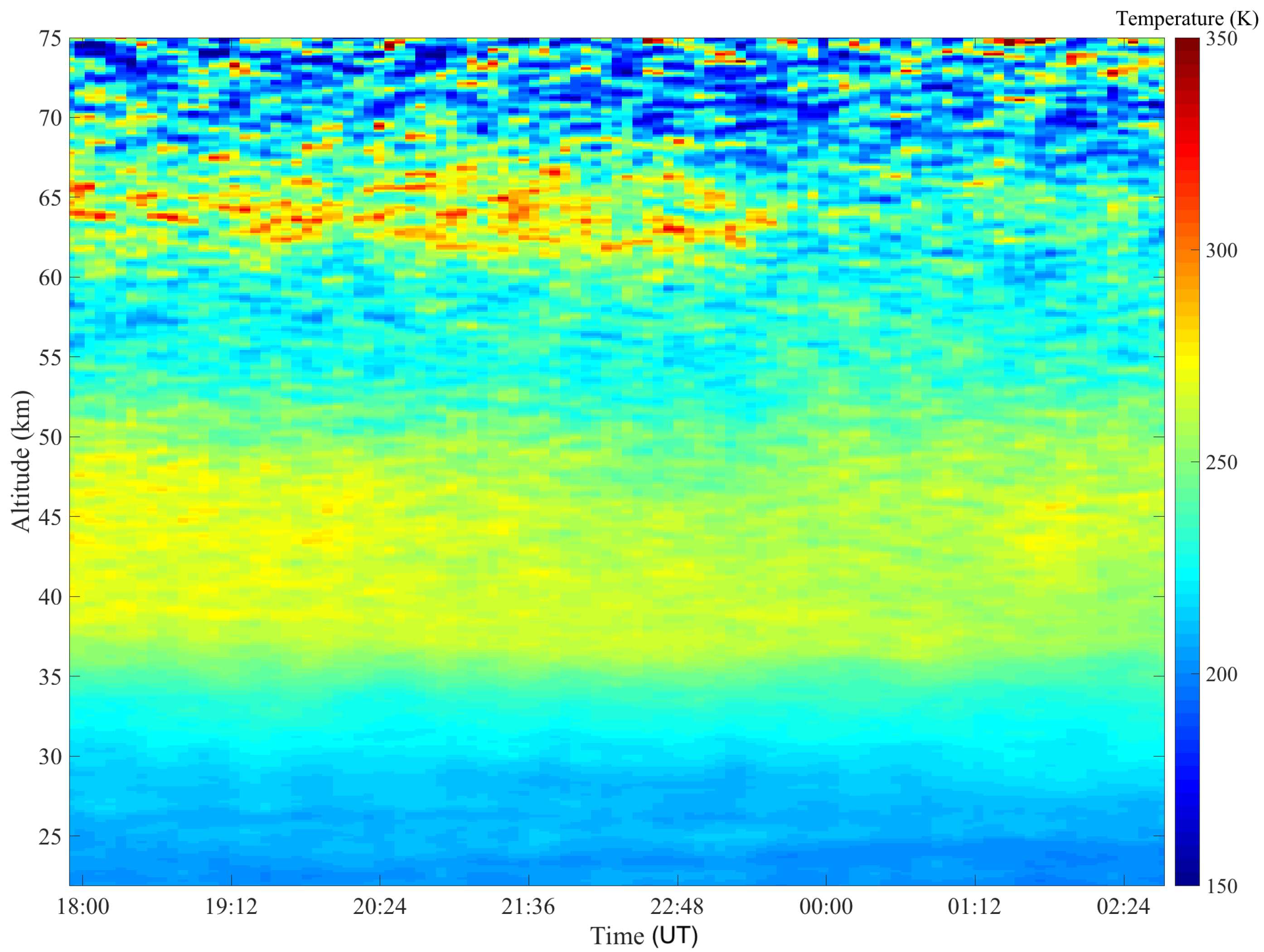
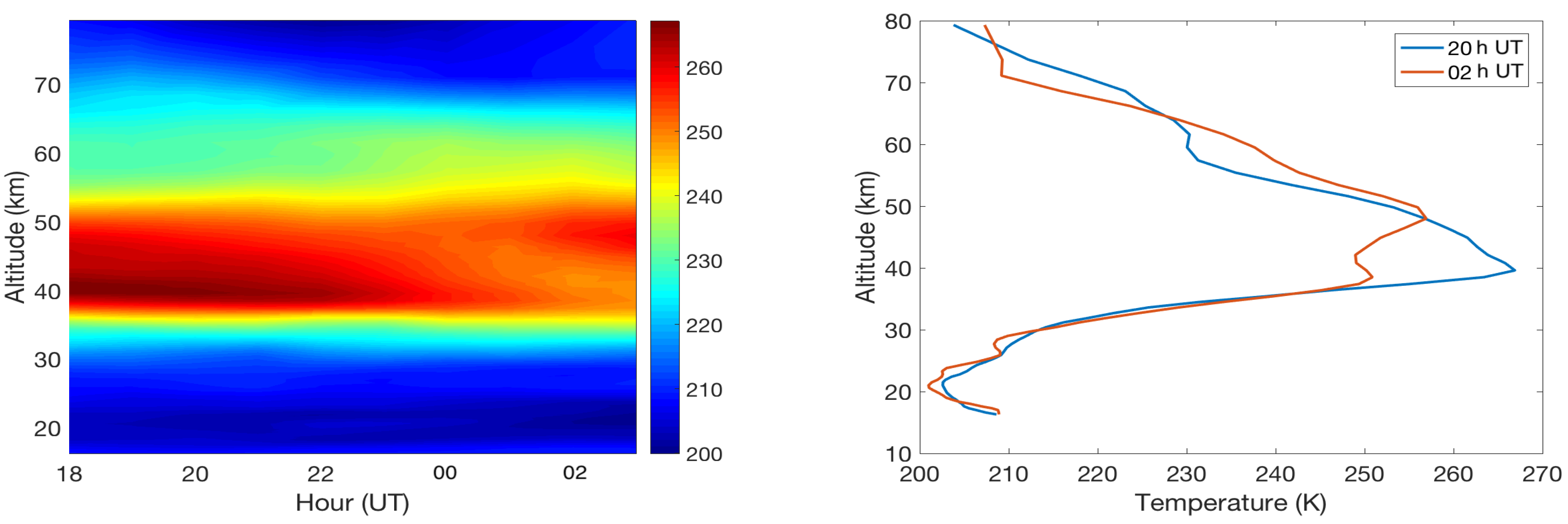
4.1. Lidar Data Analysis

During the campaign, the continuous lidar measurements allowed us to derive the vertical temperature profile from 6 pm to 3 am with a temporal resolution of one minute and a vertical resolution of 0.150 km. This allowed us to observe the occurrence of a strong MIL around 65 km altitude at the beginning of the night, which partially disappears around midnight (Figure 9). This behavior is also noticeable on the square Brunt–Väisälä frequency profiles deduced from the lidar temperature profiles, which show convective instabilities occurred at 50 km altitude and were even more pronounced at 68 km altitude, where N² is negative (Figure 9). To obtain the N² profile, each lidar temperature profile was averaged using a 4.5 km sliding-average window. In the same way, a sliding-average was applied to the potential temperature (window length = 3 km) to reduce noise at high altitude. We observed negative values during the whole period when the MIL is present, turning to positive values after, leading to a relatively higher stability after midnight. These negative values during the first part of the night were due to the strong negative temperature gradient caused by the MIL (Figure 9). The largest values are located at the top part of the MIL (Figure 9). It has been shown from numerical simulation that large-amplitude GWs encountering the MIL are trapped and achieve large amplitudes and shears within the MIL [28].

MILs are characterized by a negative atmospheric lapse rate value ($\mathsf{\Gamma }=-\partial T/\partial z$), in contrast to the positive value usually observed between the stratopause and mesopause. Its persistence can be explained by the heating of the turbulent layers generated by the continuous breaking of gravity waves above the secondary minimum of temperature [12]. Indeed, a MIL appears to be a signature of wave breaking in the mesosphere, and some studies have shown that, statistically, MILs occur most often in winter [44]. The amplitude of the inversions is directly associated with the amplitude of the planetary waves, to such an extent that large inversions develop during planetary wave amplification episodes. Sassi et al. [45] suggests that gravity waves play an indirect role in the formation of inversions because their breaking occurs above the range of altitudes where the inversions are located.

The mesospheric inversion is also observed on the ERA5 data interpolated above the OHP location (Figure 10, right). The MIL appears on the model at the same altitude as lidar (around 60 km altitude) with a similar temporal behavior. The MIL amplitude is, however, smoother than the measured data by a factor of approximately 10.

In order to estimate gravity wave activity and its vertical evolution, a method based on the variance of the lidar signal [11] is applied, where the altitude evolution of the potential energy Ep per unit mass (J/Kg) is computed:

$$E_p=\frac{1}{2}\frac{g^2}{N^2}{\left(\frac{T^{\prime }}{T}\right)}^2$$

(5)

where $T^{\prime }$ is the temperature perturbation induced by gravity waves and T the night averaged temperature. Calculating temperature fluctuations involves smoothing each individual temperature profile and subtracting them from the average night profile [11].

These estimates were calculated using lidar signals for the time periods before and after midnight (Figure 11) according to the mesospheric inversion appearance. We notice that the loss of wave energy does not occur at the same altitudes during and after the MIL. The calculated potential energy shows a decrease from 50 to 58 km altitude, when mesospheric inversion was present; this decrease was not significantly observed when it disappeared. The waves losing energy may have contributed to the formation of the MIL and maintained it for several hours. Before midnight, the potential energy density increased from 58 to 64 km altitude and seemed to increase again above 64 km altitude. The latter increase may be due to the generation of secondary GWs within the inversion that propagated up to the lower thermosphere [26]. The MIL is a favorable region for the breaking of upward propagating GWs. As shown by Hauchecorne et al. [12], the positive temperature gradient within the MIL leads to an increase in the amplitude of GWs and a decrease in their wavelength, which leads to dynamical instabilities, GW breaking, and the generation of secondary GWs. We noticed that potential energy increased slightly from 40 to 45 km altitude after midnight, probably associated with the reinforcement of the wind observed at this altitude in meteorological analyses. This increase of wave activity could have induced the strong breaking above between 50–58 km altitude and the MIL.

In order to analyze the frequency of temperature disturbances at the place and time when the potential energy is decreasing, the Fourier spectrum is investigated using the same method as described in Section 3.1 (Figure 4) but this time dividing the time domain into two parts, during and after midnight (Figure 12). Individual lidar temperature profiles were filtered with a low-pass filter with a 1/800 m cut-off frequency in order to reduce noise. The average night profile is filtered in the same way with a 1/4 km cut-off frequency, and this average profile is subtracted from each individual profile.

We notice that small periods have a lot of energy in each case, exceeding the 99% confidence level. For the altitude range [42–48] km (Figure 12), there are several peaks between 2 and 3.5 min for the spectrum after midnight (no inversion), which is consistent with turbulence generated by the decrease of the potential energy curve. Conversely, for the altitude range [50–58] km (Figure 12), there is a 4 min period in the spectrum during the inversion that is consistent with turbulence generated by the MIL. These peaks could be due to the breaking of gravity waves, which causes turbulence.

It is also interesting to analyze the impact of gravity waves on wind behavior. As gravity waves interact with the mean flow during a drop in potential energy, the local wind speed is impacted, as shown in Figure 13. Indeed, the ERA5 data show a progressive descent of the local maximum wind speed during the night; this phenomenon is clearly visible by looking at the divergence of the wind speed. The air has to descend into the inversion to create adiabatic warming, so convergence is expected above the inversion and divergence below, as shown in Figure 13. Figure 13 also shows the vertical wind speed (w expressed in Pa.s⁻¹) divided by the pressure (p). Before midnight, the positive vertical speed around 50 km altitude (w/p < 0) and the negative vertical speed above 65 km altitude (w/p > 0) contribute to creating the MIL. Adiabatic cooling occurs below and adiabatic heating above, which increases the vertical gradient of temperature (dT/dz > 0). The opposite after midnight will contribute to the disappearance of the MIL [12].

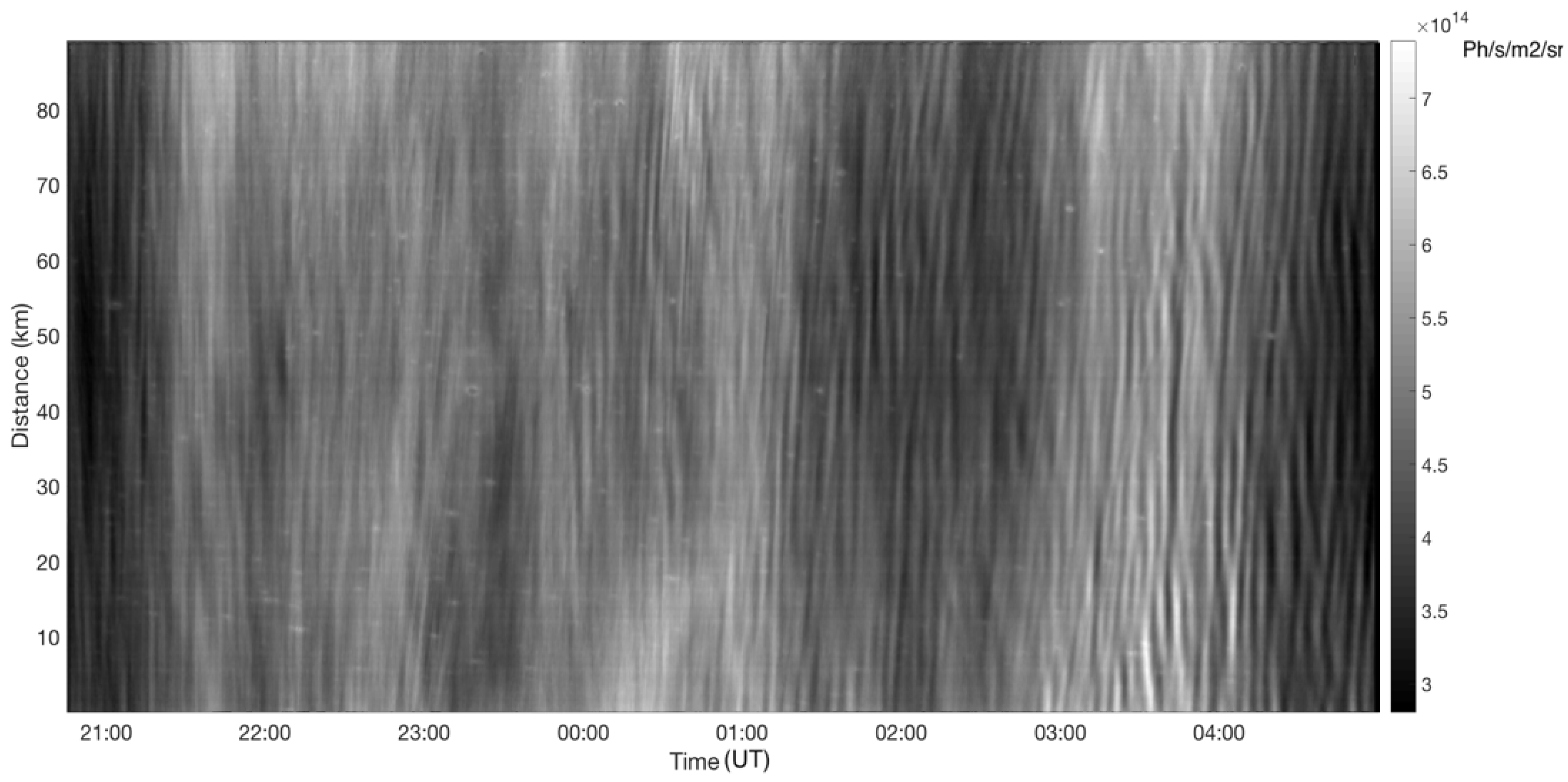
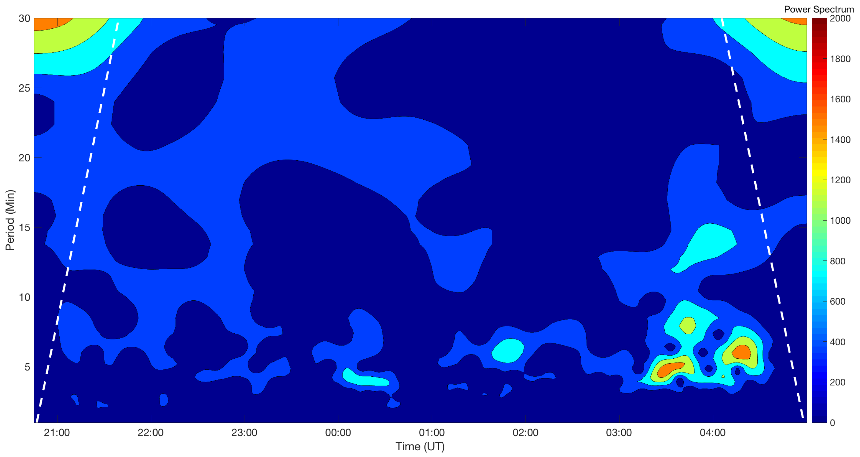
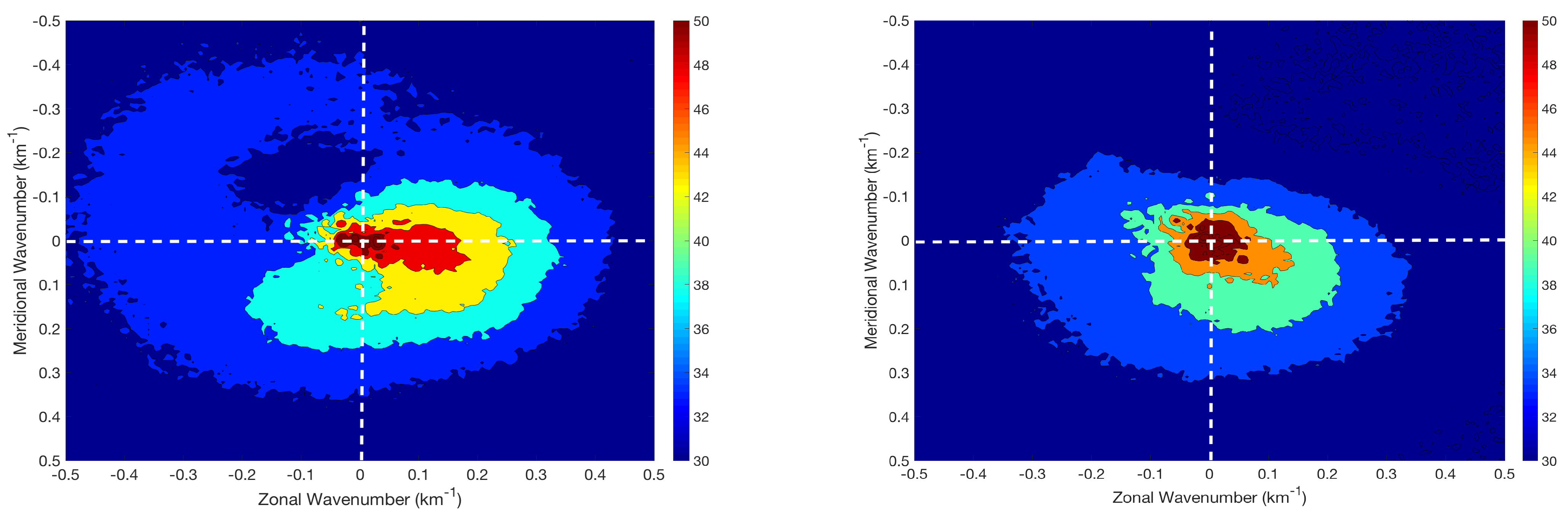
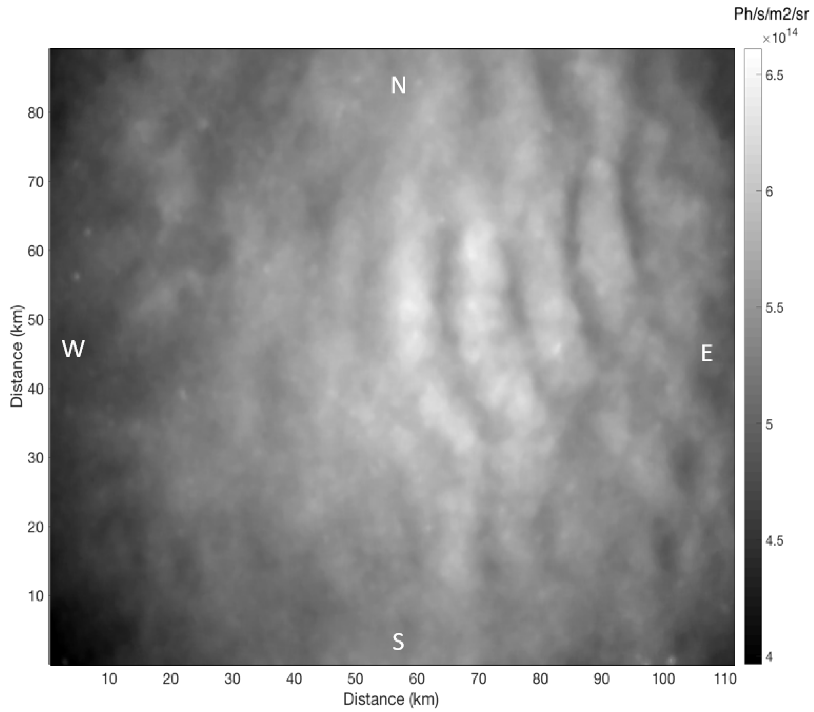
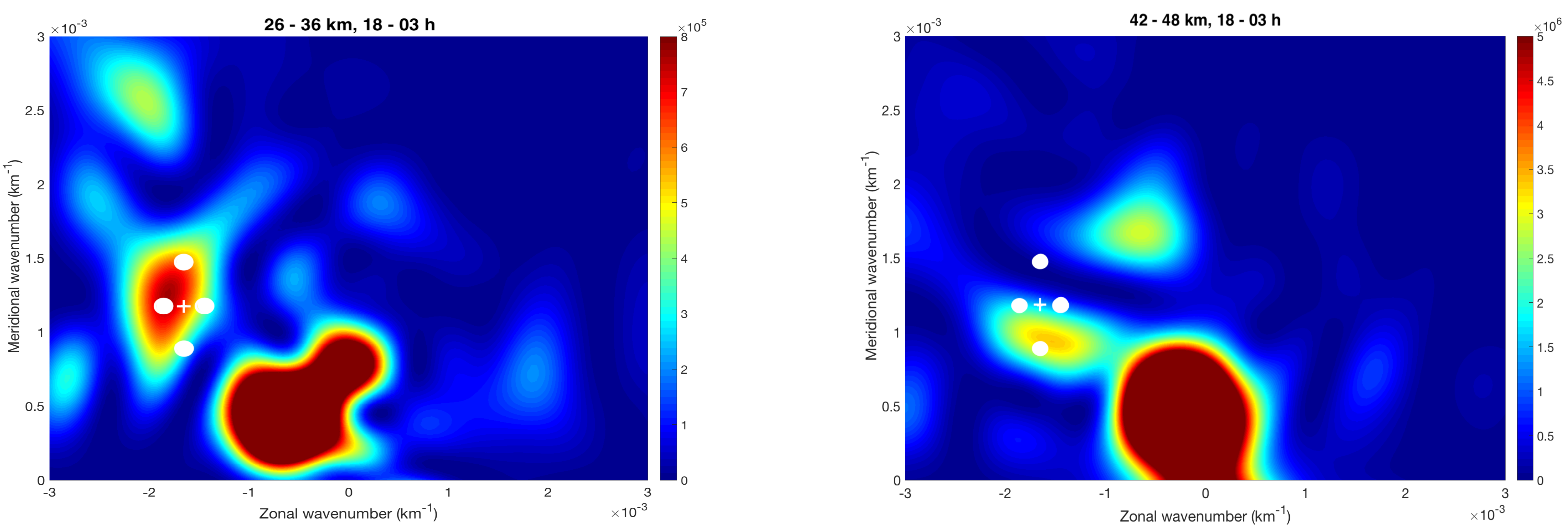
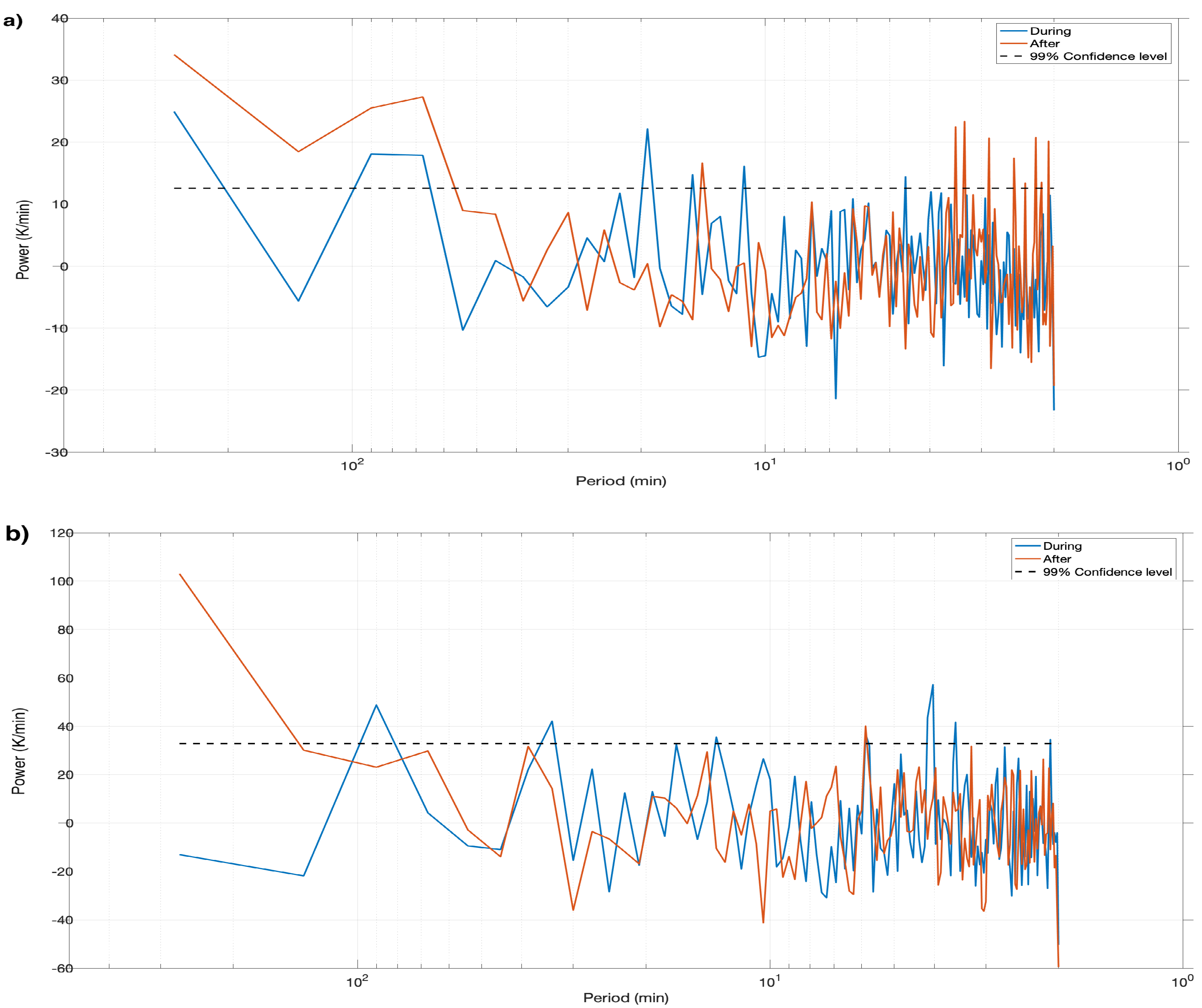
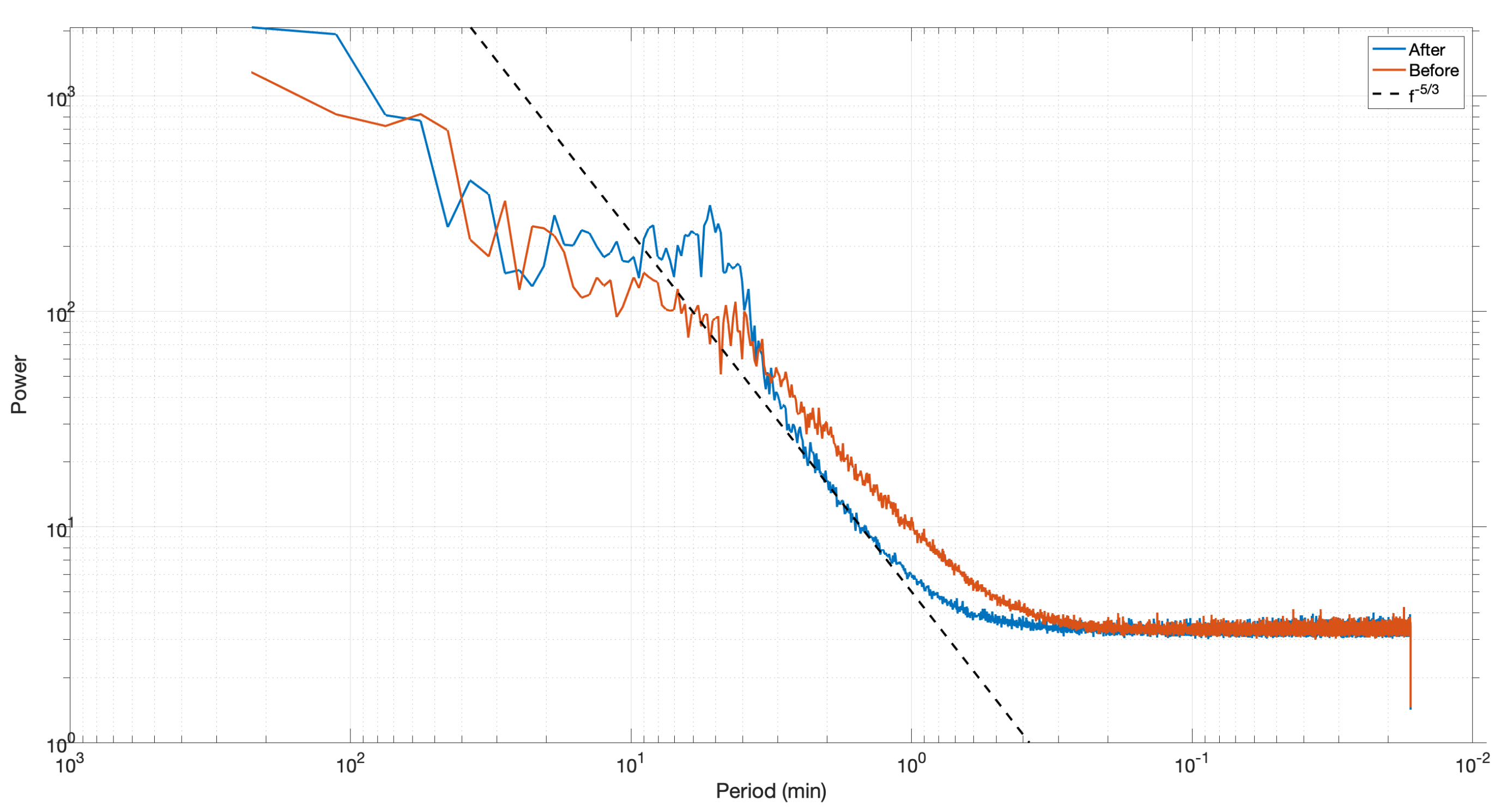
4.2. OH Airglow Images Analysis

To investigate wave evolution above the mesospheric inversion layer, the OH observations were analyzed. The camera acquired images from 20h 45 UT until 05 h UT at two frames per second. Figure 2 shows an example of a corrected image acquired during the night. The analysis of these separated images consists of the determination of the temporal evolution of the radiance during the entire night. In order to improve signal-to-noise ratio, a matrix of five by five pixels is selected at the center of each image and averaged to provide the mean OH radiance temporal profile. A Morlet wavelet analysis is applied to this time series (Figure 14).

We note the appearance of periods between 5 and 15 min after midnight, which intensify at the end of the night. This is probably due to the presence of the MIL before midnight, which prevents the small-scale gravity waves from reaching the OH layer. This behavior might be also observed with a keogram analysis as performed in Section 3.1. A Fourier transform to the north–south keogram was performed in order to analyze the frequency content of the night, with signals separated in the two periods (Figure 15). If we compare before and after midnight, there is a fairly clear difference in energy between 0.4 and 3 min in Figure 15, which can be explained by the possible generation of turbulence with high wavenumber caused by the breaking waves. Indeed, the MIL is most probably causing this breaking process. The second half of the night has more energy between 5 and 20 min. Indeed, gravity waves reach the OH layer more easily in the absence of the MIL. However, this analysis concerns only a small part of each image. A more accurate way to perform the analysis is to calculate the two-dimensional unambiguous horizontal wavenumber spectra for the two parts of the night. To do this, the images must be pre-processed, as described in Coble et al. [46]. To reduce the spectral distortion, the normalized images are prewhitened spatially by using a filter whose coefficients are given in Coble et al. [46], and a 2D Hanning window ($\alpha$ = 0.5) is applied to the data before computing the spectrum. For the calculation, we use a cube of 450 images with a temporal resolution of 30 s for each part of the night.

The unambiguous horizontal wavenumber spectra show the energy distribution of gravity waves as a function of the direction of propagation as well as zonal and meridional wavenumbers (Figure 16). The preferred direction of propagation of gravity waves during the night is southeast. The spectrum of the first part of the night has more energy in high wavenumbers than the spectrum of the second part of the night. These short wavelengths propagate in any direction and may result from non-linear interactions caused by the MIL and can generate turbulence. It may be noted that the spectrum of the second part of the night has more energy in the low wavenumbers; it can be deduced that these waves can propagate freely due to the disappearance of the MIL. By measuring the horizontal wavelength and phase velocity of these waves directly on the raw images, we obtain the 5 and 15 min periods as in the wavelet analysis.

5. Conclusions and Discussion

The objective of the study was to use a varied set of tools and observations to analyze gravity wave propagation through the perturbed mesosphere during an MIL.

This study is a first attempt to use the opportunity of the MIL occurrence to better understand the impact of the background atmosphere on the vertical propagation of gravity waves. The previous specific studies of Fritts et al. [28,29] using numerical simulations provide a detailed theoretical background that helps to appreciate verifications using the observations. Despite the fact that these two studies use only short periods for gravity waves (from 417 to 509 s), we can note some common conclusions. The theoretical study shows an increased transmission for long wavelengths as well as the creation of turbulence due to the breaking of gravity waves in the MIL. Our study has shown that long wavelengths are weakly impacted by the MIL compared to short wavelengths (∼ 10%), as shown in Figure 16. We also note the presence of energy in the short wavelengths above the inversion (87 km) as shown in Figure 16, which suggests additional local wave generation may be induced by the turbulence process. Finally, the potential energy of gravity waves is reduced threefold below the inversion (∼55 km) but is increased 15 times more at the inversion level (∼60 km), which shows the importance of wave regeneration (Figure 11).

OH spectra of gravity waves at 87 km (Figure 6) show some enhanced periods, such as one at 150 min, which are also included in the energy band of the spectrum in the mid-stratosphere (Figure 4). Using the HWM07 model to compute the local wind, GW horizontal wavelengths of several hundred kilometers were determined. Note that wind estimation did not allow accurate intrinsic waves characteristics, as tides are not well represented in the HWM07 model by a factor of 2. Furthermore, such large scale waves are also observed in the stratosphere in ERA5 meteorological analyses. The mesospheric inversion observed in lidar data, corresponding to a nearly undetectable anomaly on ERA5, is associated with gravity wave energy dissipation just below the MIL by a factor of nearly 10 and regenerating instabilities above with a similar energy amount. During the period when the MIL is not observed, wave energy dissipation occurs at lower altitude (40–50 km) by a factor of 5, probably due to enhanced wind at this altitude, causing MIL disappearance, and then gravity waves propagate freely from 50 to 70 km with very small waves mean flow interactions. At 87 km, OH images analysis shows that large scale gravity waves are reduced during the period when MILs exist. This is in agreement with the potential energy dissemination reported by the lidar observations, whereas the smaller scale gravity wave observed at the same time were probably generated in the upper part of the MIL, leading to a cascade redistribution of wave energy.

This work concerns only one night of observations. We plan to carry out further measurement campaigns in order to establish statistical results on the impact of an MIL on gravity waves propagation. This work made it possible, on the one hand, to point out the impact of an MIL on the propagation of gravity waves and, on the other hand, to follow the propagation of one of them by associating the Rayleigh lidar, the airglow cameras, and the ERA5 re-analysis. The study also shows an approach for the determination of intrinsic gravity wave parameters from keograms.

References

1. Hamilton, K. Comprehensive meteorological modelling of the middle atmosphere: A tutorial review. J. Atmos. Terr. Phys. 1996, 58, 1591–1627. [Google Scholar] [CrossRef]
2. Holton, J.R. The role of gravity wave induced drag and diffusion in the momentum budget of the mesosphere. J. Atmos. Sci. 1982, 39, 791–799. [Google Scholar] [CrossRef] [Green Version]
3. Fritts, D.C.; Alexander, M.J. Gravity wave dynamics and effects in the middle atmosphere. Rev. Geophys. 2003, 41, 1–63. [Google Scholar] [CrossRef] [Green Version]
4. Taylor, M.J.; Hapgood, M. Identification of a thunderstorm as a source of short period gravity waves in the upper atmospheric nightglow emissions. Planet. Space Sci. 1988, 36, 975–985. [Google Scholar] [CrossRef]
5. Chane Ming, F.; Ibrahim, C.; Barthe, C.; Jolivet, S.; Keckhut, P.; Liou, Y.A.; Kuleshov, Y. Observation and a numerical study of gravity waves during tropical cyclone Ivan (2008). Atmos. Chem. Phys. 2014, 14, 641–658. [Google Scholar] [CrossRef] [Green Version]
6. Alexander, M.J.; May, P.T.; Beres, J.H. Gravity waves generated by convection in the Darwin area during the Darwin Area Wave Experiment. J. Geophys. Res. Atmos. 2004, 109, D20S04. [Google Scholar] [CrossRef]
7. De la Cámara, A.; Lott, F. A parameterization of gravity waves emitted by fronts and jets. Geophys. Res. Lett. 2015, 42, 2071–2078. [Google Scholar] [CrossRef]
8. Becker, E.; Schmitz, G. Climatological effects of orography and land–sea heating contrasts on the gravity wave–driven circulation of the mesosphere. J. Atmos. Sci. 2003, 60, 103–118. [Google Scholar] [CrossRef]
9. Hickey, M.P.; Schubert, G.; Walterscheid, R. Propagation of tsunami-driven gravity waves into the thermosphere and ionosphere. J. Geophys. Res. Space Phys. 2009, 114. [Google Scholar] [CrossRef]
10. Lindzen, R.S. Turbulence and stress owing to gravity wave and tidal breakdown. J. Geophys. Res. Ocean. 1981, 86, 9707–9714. [Google Scholar] [CrossRef] [Green Version]
11. Mzé, N.; Hauchecorne, A.; Keckhut, P.; Thétis, M. Vertical distribution of gravity wave potential energy from long-term Rayleigh lidar data at a northern middle-latitude site. J. Geophys. Res. Atmos. 2014, 119, 12–69. [Google Scholar] [CrossRef]
12. Hauchecorne, A.; Chanin, M.L.; Wilson, R. Mesospheric temperature inversion and gravity wave breaking. Geophys. Res. Lett. 1987, 14, 933–936. [Google Scholar] [CrossRef]
13. Chanin, M.L.; Hauchecorne, A. Lidar observation of gravity and tidal waves in the stratosphere and mesosphere. J. Geophys. Res. Oceans 1981, 86, 9715–9721. [Google Scholar] [CrossRef]
14. Rauthe, M.; Gerding, M.; Lübken, F.J. Seasonal changes in gravity wave activity measured by lidars at mid-latitudes. Atmos. Chem. Phys. 2008, 8, 6775–6787. [Google Scholar] [CrossRef] [Green Version]
15. Wilson, R.; Chanin, M.; Hauchecorne, A. Gravity waves in the middle atmosphere observed by Rayleigh lidar: 1. Case studies. J. Geophys. Res. Atmos. 1991, 96, 5153–5167. [Google Scholar] [CrossRef]
16. Baker, D.J.; Stair, A., Jr. Rocket measurements of the altitude distributions of the hydroxyl airglow. Phys. Scr. 1988, 37, 611. [Google Scholar] [CrossRef]
17. Swenson, G.R.; Mende, S.B. OH emission and gravity waves (including a breaking wave) in all-sky imagery from Bear Lake, UT. Geophys. Res. Lett. 1994, 21, 2239–2242. [Google Scholar] [CrossRef]
18. Taylor, M.J.; Bishop, M.; Taylor, V. All-sky measurements of short period waves imaged in the OI (557.7 nm), Na (589.2 nm) and near infrared OH and O2 (0, 1) nightglow emissions during the ALOHA-93 campaign. Geophys. Res. Lett. 1995, 22, 2833–2836. [Google Scholar] [CrossRef] [Green Version]
19. Smith, S.M.; Mendillo, M.; Baumgardner, J.; Clark, R.R. Mesospheric gravity wave imaging at a subauroral site: First results from Millstone Hill. J. Geophys. Res. Space Phys. 2000, 105, 27119–27130. [Google Scholar] [CrossRef]
20. Le Du, T.; Simoneau, P.; Keckhut, P.; Hauchecorne, A.; Le Pichon, A. Investigation of infrasound signatures from microbaroms using OH airglow and ground-based microbarometers. Adv. Space Res. 2020, 65, 902–908. [Google Scholar] [CrossRef]
21. Pautet, P.D.; Taylor, M.J.; Pendleton, W.; Zhao, Y.; Yuan, T.; Esplin, R.; McLain, D. Advanced mesospheric temperature mapper for high-latitude airglow studies. Appl. Opt. 2014, 53, 5934–5943. [Google Scholar] [CrossRef] [PubMed] [Green Version]
22. Sivakandan, M.; Taori, A.; Sathishkumar, S.; Jayaraman, A. Multi-instrument investigation of a mesospheric gravity wave event absorbed into background. J. Geophys. Res. Space Phys. 2015, 120, 3150–3159. [Google Scholar] [CrossRef]
23. Taylor, M.J.; Gu, Y.; Tao, X.; Gardner, C.; Bishop, M. An investigation of intrinsic gravity wave signatures using coordinated lidar and nightglow image measurements. Geophys. Res. Lett. 1995, 22, 2853–2856. [Google Scholar] [CrossRef] [Green Version]
24. Lossow, S.; McLandress, C.; Jonsson, A.I.; Shepherd, T.G. Influence of the Antarctic ozone hole on the polar mesopause region as simulated by the Canadian Middle Atmosphere Model. J. Atmos. Sol.-Terr. Phys. 2012, 74, 111–123. [Google Scholar] [CrossRef] [Green Version]
25. Lubis, S.W.; Omrani, N.E.; Matthes, K.; Wahl, S. Impact of the Antarctic ozone hole on the vertical coupling of the stratosphere–mesosphere–lower thermosphere system. J. Atmos. Sci. 2016, 73, 2509–2528. [Google Scholar] [CrossRef]
26. Becker, E.; Vadas, S.L. Secondary gravity waves in the winter mesosphere: Results from a high-resolution global circulation model. J. Geophys. Res. Atmos. 2018, 123, 2605–2627. [Google Scholar] [CrossRef]
27. Okui, H.; Sato, K.; Koshin, D.; Watanabe, S. Formation of a mesospheric inversion layer and the subsequent elevated stratopause associated with the major stratospheric sudden warming in 2018/19. J. Geophys. Res. Atmos. 2021, 126, e2021JD034681. [Google Scholar] [CrossRef]
28. Fritts, D.C.; Laughman, B.; Wang, L.; Lund, T.S.; Collins, R.L. Gravity wave dynamics in a mesospheric inversion layer: 1. Reflection, trapping, and instability dynamics. J. Geophys. Res. Atmos. 2018, 123, 626–648. [Google Scholar] [CrossRef] [Green Version]
29. Fritts, D.C.; Wang, L.; Laughman, B.; Lund, T.S.; Collins, R.L. Gravity wave dynamics in a mesospheric inversion layer: 2. Instabilities, turbulence, fluxes, and mixing. J. Geophys. Res. Atmos. 2018, 123, 649–670. [Google Scholar] [CrossRef]
30. Blanc, E.; Ceranna, L.; Hauchecorne, A.; Charlton-Perez, A.; Marchetti, E.; Evers, L.G.; Kvaerna, T.; Lastovicka, J.; Eliasson, L.; Crosby, N.B.; et al. Toward an improved representation of middle atmospheric dynamics thanks to the ARISE project. Surv. Geophys. 2018, 39, 171–225. [Google Scholar] [CrossRef] [Green Version]
31. Hauchecorne, A.; Chanin, M.L. Density and temperature profiles obtained by lidar between 35 and 70 km. Geophys. Res. Lett. 1980, 7, 565–568. [Google Scholar] [CrossRef]
32. Hauchecorne, A.; Chanin, M.; Keckhut, P.; Nedeljkovic, D. Lidar monitoring of the temperature in the middle and lower atmosphere. Appl. Phys. B 1992, 55, 29–34. [Google Scholar] [CrossRef]
33. Keckhut, P.; Hauchecorne, A.; Chanin, M. Midlatitude long-term variability of the middle atmosphere: Trends and cyclic and episodic changes. J. Geophys. Res. Atmos. 1995, 100, 18887–18897. [Google Scholar] [CrossRef]
34. Beig, G.; Keckhut, P.; Lowe, R.P.; Roble, R.; Mlynczak, M.; Scheer, J.; Fomichev, V.; Offermann, D.; French, W.; Shepherd, M.; et al. Review of mesospheric temperature trends. Rev. Geophys. 2003, 41, 1–41. [Google Scholar] [CrossRef] [Green Version]
35. Kurylo, M.J. Network for the detection of stratospheric change. Remote Sens. Atmos. Chem. 1991, 1491, 168–174. [Google Scholar]
36. Drob, D.; Emmert, J.; Crowley, G.; Picone, J.; Shepherd, G.; Skinner, W.; Hays, P.; Niciejewski, R.; Larsen, M.; She, C.; et al. An empirical model of the Earth’s horizontal wind fields: HWM07. J. Geophys. Res. Space Phys. 2008, 113, A12304. [Google Scholar] [CrossRef]
37. Kawamura, S.; Otsuka, Y.; Zhang, S.R.; Fukao, S.; Oliver, W. A climatology of middle and upper atmosphere radar observations of thermospheric winds. J. Geophys. Res. Space Phys. 2000, 105, 12777–12788. [Google Scholar] [CrossRef]
38. Lukianova, R.; Kozlovsky, A.; Lester, M. Climatology and inter-annual variability of the polar mesospheric winds inferred from meteor radar observations over Sodankylä (67N, 26E) during solar cycle 24. J. Atmos. Sol.-Terr. Phys. 2018, 171, 241–249. [Google Scholar] [CrossRef]
39. Zhao, G.; Liu, L.; Wan, W.; Ning, B.; Xiong, J. Seasonal behavior of meteor radar winds over Wuhan. Earth Planets Space 2005, 57, 61–70. [Google Scholar] [CrossRef] [Green Version]
40. Pokhotelov, D.; Becker, E.; Stober, G.; Chau, J.L. Seasonal variability of atmospheric tides in the mesosphere and lower thermosphere: Meteor radar data and simulations. Ann. Geophys. 2018, 36, 825–830. [Google Scholar] [CrossRef] [Green Version]
41. Korotyshkin, D.; Merzlyakov, E.; Sherstyukov, O.; Valiullin, F. Mesosphere/lower thermosphere wind regime parameters using a newly installed SKiYMET meteor radar at Kazan. Adv. Space Res. 2019, 63, 2132–2143. [Google Scholar] [CrossRef]
42. Drob, D.P.; Emmert, J.T.; Meriwether, J.W.; Makela, J.J.; Doornbos, E.; Conde, M.; Hernandez, G.; Noto, J.; Zawdie, K.A.; McDonald, S.E.; et al. An update to the Horizontal Wind Model (HWM): The quiet time thermosphere. Earth Space Sci. 2015, 2, 301–319. [Google Scholar] [CrossRef]
43. Nappo, C.J. An Introduction to Atmospheric Gravity Waves; Academic Press: Cambridge, MA, USA, 2013. [Google Scholar]
44. Sica, R.; Argall, P.; Shepherd, T.; Koshyk, J. Model-measurement comparison of mesospheric temperature inversions, and a simple theory for their occurrence. Geophys. Res. Lett. 2007, 34, L23806. [Google Scholar] [CrossRef] [Green Version]
45. Sassi, F.; Garcia, R.; Boville, B.; Liu, H. On temperature inversions and the mesospheric surf zone. J. Geophys. Res. Atmos. 2002, 107, ACL-8. [Google Scholar] [CrossRef]
46. Coble, M.; Papen, G.C.; Gardner, C.S. Computing two-dimensional unambiguous horizontal wavenumber spectra from OH airglow images. IEEE Trans. Geosci. Remote Sens. 1998, 36, 368–382. [Google Scholar] [CrossRef]
Figure 1. The 2D temperature profile measured by the OHP Rayleigh lidar during the night of 12–13 December 2017.
Atmosphere 13 01003 g001
Figure 2. Corrected image of the OH radiation at 87 km altitude acquired during the night of 12–13 December 2017 [20]. The radiance scale is in ph/s/m2/sr. North is at the top of the image, west is on the left.
Atmosphere 13 01003 g002
Figure 3. Horizontal field of anomaly temperature extracted from ERA5 re-analysis during the night of 12–13 December 2017 at 18 h UT over Western Europe around 49 km altitude.
Atmosphere 13 01003 g003
Figure 4. Mean Fourier spectrum of lidar data for altitude range [21–32] km in blue and [32–42] km in red. The black dashed line gives the 0.95 confidence level.
Atmosphere 13 01003 g004
Figure 5. North–south keogram for the night of 12–13 December 2017 composed from a series of OH images. The grey scale is in ph/s/m2/sr.
Atmosphere 13 01003 g005
Figure 6. Mean Fourier spectrum of the entire night for the two keograms. The black dashed line is the −5/3 power law; L is the radiance unit measured on the OH images (ph/s/m2/sr).
Atmosphere 13 01003 g006
Figure 7. Temporal phase evolution of the 150 min wave extracted from the east–west keogram; the red line is the linear fit.
Atmosphere 13 01003 g007
Figure 8. Left: Average 2D Fourier spectrum of ERA 5 temperature fields for the altitude range 26–36 km (left) and 42–48 km (right) for the time range [18 p.m. 03 a.m.]. The white crosses represent the wavenumbers estimated using the OH keograms. The crosses are the estimated errors on the wavenumbers, calculated directly from the error on the slope of the linear fit (Figure 7).
Atmosphere 13 01003 g008
Figure 9. (a) Rayleigh lidar temperature profiles. The blue curve represents the average temperature for each altitude before midnight, and the red curve is the average temperature after midnight [20]. (b) Square Brunt–Väisälä frequency profile during the night of 12 December 2017 at the Haute-Provence observatory. White dots show negative values. (c) Mean square Brunt–Väisälä frequency profile before midnight in blue and after midnight in red. The 0 value is indicated by the dotted black vertical line.
Atmosphere 13 01003 g009
Figure 10. Left: 2D temperature profile during the night of 12 December 2017 from the ERA5 data. Right: Temperature profile at 20 h UT in blue and 02 h UT in red from the ERA5 data.
Atmosphere 13 01003 g010
Figure 11. Evolution of potential energy with altitude before midnight (blue curve) and after (red curve). The shaded areas are the associated errors. Adapted from [11].
Atmosphere 13 01003 g011
Figure 12. (a) Mean Fourier spectra of lidar data before and after midnight for the altitude range [42–48] km. (b) Mean Fourier spectra of lidar data before and after midnight for the altitude range [50–58] km.
Atmosphere 13 01003 g012
Figure 13. (a) Meridional wind speed in m.s−1 from ERA5 data. (b) Divergence of wind speed in s−1 from ERA5 data. (c) Vertical wind speed (in Pa.s−1 divided by pressure (in Pa)).
Atmosphere 13 01003 g013
Figure 14. Contour plot of the wavelet analysis of the temporal OH radiance profile. The white dashed lines represent the cone of influence that delimits the real periods of the discontinuities.
Atmosphere 13 01003 g014
Figure 15. Mean Fourier spectrum for the two parts of the night (before and after midnight).
Atmosphere 13 01003 g015
Figure 16. Left: Unambiguous horizontal wavenumber spectra (UHWS) from the OH images of the first part of the night, before midnight. Right: UHWS of the second part of the night, after midnight. The color bar in the 2D spectra is in logarithmic scale and represents the square of the magnitude (cyc/m)2. White dashed lines show the position of the zero wavenumbers.
Atmosphere 13 01003 g016