Abstract
Soil moisture (SM) plays an important role in regulating terrestrial–atmospheric water circulation and energy balance. Most of the existing studies have explored the dynamic patterns of SM based on experimental methods. However, the analysis of large-scale regions and long-term SM sequences was limited. Alternatively, satellite remote sensing data is a potential source for SM analysis for large-scale basins. Therefore, the SM data from the European Space Agency (ESA) Climate Change Initiative (CCI) from 2000 to 2015 is used in this paper to analyze the SM spatial-temporal changes in the Yellow River Basin (YRB). Further, the Normalized Difference Vegetation Index (NDVI) and meteorological data are used to explore the relationships between SM and NDVI, precipitation, air temperature, and wind speed, respectively. The results showed that the overall trend of SM in the YRB was decreasing from southeast to northwest during the past 16 years. The upper reaches of the YRB had shown a humid trend, with a value of 0.00047 m3·m−3·year−1, mainly due to the increase in precipitation; there was an obvious drought trend in the middle reaches of the YRB, especially in Shanxi Province and Henan Province, with a value of −0.00030 m3·m−3·year−1, which may be owed to vegetation greening increasing the soil evaporation. Overall, it is determined that the main factors influencing SM changes were NDVI and precipitation, followed by air temperature and wind speed. This study can provide a scientific basis for the spatial-temporal distribution characteristics and attributions of SM in the YRB over a long time series.
1. Introduction
Soil moisture (SM), as an important component of soil, is one of the important variables for characterizing land surface conditions and plays a significant role in regulating the terrestrial–atmospheric water cycle and energy balance [1,2,3,4]. SM controls the infiltration rate, thus influencing runoff [5], and also affects the conversion process of latent and sensible heat at the surface [6]. In arid and semi-arid areas, SM is an important indicator reflecting vegetation growth conditions and agricultural drought [7,8]. The long-term shortage of SM may lead to the imbalance of energy exchange between the surface and the atmosphere and further cause the deterioration of the regional ecological environment [9]. Therefore, an accurate grasp of the spatial-temporal characteristics and attributions of SM is beneficial for monitoring and early warning of drought.
The traditional SM monitoring methods mostly use the oven-drying method [10], which can measure the SM content at different depths with high accuracy, but there are shortcomings, such as high sampling cost, time-consuming and laborious, and point substituting surface, which cannot achieve dynamic monitoring of large areas. In recent years, with the rapid development in the field of remote sensing, it has become possible to monitor SM in real-time and dynamically based on satellite remote sensing. Microwave remote sensing has established its dominant position in SM monitoring because it is not affected or rarely affected by cloud, rain, and fog, does not need lighting conditions, and can obtain images and data all day and in all weather [11]. Yang et al. [12] and Liu et al. [13] found that surface SM was well correlated with deep SM through their study. Therefore, the surface SM based on remote sensing inversions can reflect the change in the whole SM to a certain extent.
In addition, the spatial-temporal variability of SM can be influenced by environmental factors and human activities, such as climate change [14], terrain [15], vegetation growth conditions [16], and irrigation. Fan et al. [17] quantitatively analyzed the contribution of precipitation, air temperature, wind speed, and other climate factors to SM change by using the multivariable generalized linear model; among them, precipitation contributed the most to SM, roughly 60–80%, while the contribution of other climate factors, such as air temperature and wind speed, was less than 40%. Ayehu et al. [18] analyzed the relationship between long-term variability of SM and precipitation in the Upper Blue Nile Basin in Ethiopia based on remote sensing data; the results showed that spatial patterns and changes of SM and precipitation were similar in this region, demonstrating that precipitation was the main driving force affecting SM variability in the region. Compared with terrain factors, vegetation coverage has a more direct and rapid effect on the spatial distribution of SM [19]. Through experimental studies, Miyamoto et al. [17] found that SM was greatly affected by vegetation conditions and that SM in fields covered by vegetation was greater than that without vegetation. However, some studies did not adequately consider the effects of these environmental factors on SM [20,21], which may lead to some uncertainties in the existing results.
The European Space Agency (ESA) Climate Change Initiative (CCI) remote sensing SM data is based on active and passive microwave sensors [22], combining the advantages of both generated and long time series (1979–2019) of active, passive, and fused datasets. As the longest remote sensing data with known time series in the world, ESA CCI SM data have received widespread attention since its release and have been effectively applied in many parts of the world. Zohaib et al. [23] evaluated global irrigation water information from 2000 to 2015 by using ESA CCI SM data, and the results showed that ESA CCI products could identify global irrigation areas well with an accuracy of about 65%, and the study found that global irrigation water in recent years has an upward trend. Tomas et al. [24] used ESA CCI products to analyze the relationship between SM and soil water storage in northeastern Portugal and established a regression model, which proved that the model had high accuracy through verification. Based on ESA CCI SM data, Wang et al. [21] studied the spatial-temporal variation of SM in the South–North Water Transfer Jiangsu water supply area from 1991 to 2019, and the results showed that the spatial distribution of SM in the area was “wet south and dry north”; in the past 29 years, SM had been on the rise as a whole. However, there are relatively few applications of ESA CCI SM data in China, and they mostly focus on small-scale research [25,26].
The Yellow River Basin (YRB) covers many dry, semi-arid areas, with large deserts and sandy areas in the north, alpine zones in the west, and a loess plateau in the center, where drought, sand, and soil erosion disasters are serious, and the ecological environment is fragile. In summary, based on the ESA CCI SM data of the YRB from 2000 to 2015, combined with NDVI and meteorological (precipitation, air temperature and wind speed) data, this paper analyzed the spatial-temporal evolution law of SM in the YRB over the past 16 years and its correlation with various environmental factors, and further results in the main control factors affecting the spatial-temporal variation of SM. This study can provide a scientific basis for the ecological construction and water resources management in the basin, helping to promote the development of ecological protection and high-quality development strategy in the YRB.
2. Materials and Methods
2.1. Study Area Overview
The YRB is located between 96–119° E and 32–42° N, with a total basin area of 7.95 million square kilometers, of which the upper, middle, and lower reaches of the basin account for 53.8%, 43.3%, and 2.9%, respectively. The YRB is bounded by Bayankala Mountain in the west, Yinshan Mountain in the north, Qinling Mountain in the south, and Bohai Sea in the east, and the terrain in the basin is high in the west and low in the east, with a huge difference in height, forming a three-step ladder from west to east, from high to low. The YRB is located in the mid-latitude zone; due to the influence of atmospheric circulation and monsoon circulation, the climate of different regions is significantly different, and the annual and seasonal variations are great. The average annual precipitation in the basin for the last 60 years is roughly 470 mm, and the seasonal distribution is very uneven, 60% of which is concentrated in June to September; the annual average air temperature is between − and 14 °C, the precipitation and air temperature decreases from southeast to northwest. The main vegetation types in the YRB are grassland, woodland, and arable land, with vegetation cover of up to 60%.
Since ancient times, the channel changes of the Yellow River have mainly occurred in the lower reaches, so this paper focuses on the study of the spatial-temporal distribution characteristics of SM in the middle and upper reaches of the YRB in recent years, as shown in Figure 1.
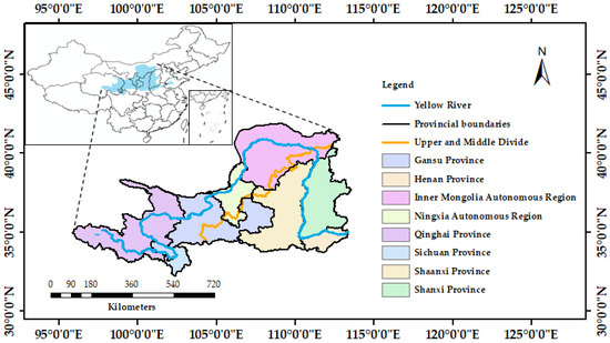
Figure 1.
The location of Yellow River Basin.
2.2. Data Sources
2.2.1. Soil Moisture Data
This study uses SM data published by the European Space Agency Climate Change Initiative, including three data products: active data set, passive data set, and active-passive fused data set. Among them, the active data set is derived from active microwave remote sensing products, such as ERS-1/2, AMI-WS, and ASCAT (Metop-A/B), and the passive data set is derived from passive microwave remote sensing products such as SMMR, DMSP SSM/1, SMOS, and TRMM TM1. The active-passive fusion data set is fused from the above two kinds of datasets. The ESA CCI SM data are provided in netcdf-4 format, with a temporal resolution of 1 d and a spatial resolution of 0.25°, the unit is m3·m−3.
The product provides SM data from 1978 to 2016, which is the longest remote sensing data with a known time series worldwide. Its validity in describing regional SM changes has been fully verified. Dorigo et al. [27] evaluated the random error of ESA CCI SM data using the triple collocation technique based on SM observations from 596 ground stations worldwide, the results showed that the absolute value of the average Spearman correlation coefficient between the two was 0.46, and the mean values of the unbiased root-mean-square differences and triple collocation errors were 0.05 and 0.04, respectively. Xu et al. [28] verified the ESA CCI SM data and field observation data in the Laurentian Great Lakes basin with a sparse network, and the results showed that the unbiased root-mean-square error of the two was 0.04 and the correlation coefficient was about 0.7. Ling et al. [29] evaluated the ESA CCI SM data and on-site observation data from 1981 to 2013 in four regions of China; the results showed that the ESA CCI SM data and on-site observation data were in good agreement, with relative root mean square errors less than 0.02 in different regions, indicating that the product is a good choice for studying long-term SM change in China.
In this paper, the ESA CCI SM product from 2000 to 2015 was selected to study SM variations, with a temporal resolution of 1 d and a spatial resolution of 0.25°.
2.2.2. Meteorological Data
The original meteorological data (precipitation, air temperature, wind speed, etc.) used in this study come from 2481 meteorological observation stations nationwide at the National Meteorological Science Data Center (http://data.cma.cn/, accessed on 20 October 2021). In this study, the meteorological data were further processed into raster data with a temporal resolution of 1 d and a spatial resolution of 0.25° using the inverse distance weight interpolation method and cropping out the values within the YRB.
2.2.3. Vegetation Coverage Data
The Normalized Difference Vegetation Index (NDVI) is one of the most commonly used vegetation indices, and its change can reflect the change in surface vegetation coverage to a certain extent. Therefore, NDVI has a wide range of applications in SM research, ecological environment protection and other fields [30]. The NDVI data used in this study comes from the National Science and Technology Resource Sharing Service Platform—National Earth System Science Data Center (http://www.geodata.cn, (accessed on 15 March 2022), the time scale is the month, and the spatial resolution is 5 km. In this study, the mask method was used to cut out data in the YRB from the national scope.
2.3. Methods
In recent years, with the maturity and application of classical statistics, geostatistics, time series analysis, and other methods, the research on soil moisture movement, heterogeneity, prediction, and influencing factors has been carried out comprehensively. Among them, the geostatistical method is one of the most common methods to determine the spatial distribution characteristics of SM [31,32]. Among the time series analysis methods, the Mann–Kendall (M-K) trend test method, as a non-parametric test method, is suitable for analyzing the overall change trend of non-normal distribution data [33,34]. Principal component analysis (PCA) is widely used to identify the main factors influencing SM variability because of its ability to retain the information of original variables [35,36,37].
Therefore, in this study, the M-K trend test methods was used to analyze the interannual variation characteristics of soil moisture, and the relationship between soil moisture and four environmental factors was explored by correlation analysis methods and PCA methods.
2.3.1. Mann–Kendall Trend Test Methods
The Mann–Kendall (M-K) trend test method is a non-parametric statistical method used to detect the trend of the sequence change. The advantage is that the calculation is simple and convenient, the human factors are small, the data are quantified, and the sample detection range is wide and does not need to obey a certain distribution and will not be interfered with few abnormal values, and it can also clear the time when the sequence begins to mutate. In this paper, based on the M-K trend test methods, MatLab programming is used to achieve the inter-annual trend test analysis of SM. The calculation principle is as follows:
For the time series x of the sample number n, construct a series:
The value of ri is as follows:
It can be seen that the series sk is the cumulative count of the number of values at time i greater than that at time j.
The statistics are defined under the assumption of random independence of the time series:
where E(sk) and var(sk) are the mean and variance of sk; UF1 = 0.
When x1, x2, …, xn are independent of each other and are continuous, they can be calculated by the following equation:
UFk is the standard orthogonal distribution, which is a statistic sequence calculated in the order of the time series x1, x2, …, xn. Then, repeat the above process in the time series inverse order xn, xn−1, …, x1 so that UBk = −UFk, UB1 = 0. In this paper, given a significance level of ɑ = 0.05 and a critical value of u0.05 = ±1.96, the two statistical series curves of UFk and UBk, the two straight lines of ±1.96, and the 0-value straight line are plotted on the same graph.
If the UFk line in the graph fluctuates between the critical lines, it indicates that the series variation trend is not significant; when the value of UFk is greater than zero, it indicates that the series has an upward trend otherwise it has a downward trend; when it exceeds the critical line, it indicates a significant upward or downward trend. If UFk and UBk have an intersection between the critical lines, the moment corresponding to the intersection is the time when the mutation begins.
2.3.2. Correlation Analysis Methods
In this study, correlation analysis methods were used to analyze the correlation between SM and climatic factors from NDVI in the YRB. The correlation coefficient is a statistic used to describe the degree and direction of linear correlation between two variables, usually denoted by r. The specific expression is as follows:
where rxy is the correlation coefficient of variable x and variable y; n is the number of samples; and , is the mean of variable x and variable y, respectively.
The r-value is between −1 and 1. When r > 0, it indicates that the two are positively correlated, the closer r-value is to 1, the more significant the positive correlation is; when r < 0, it indicates that the two are negatively correlated, the closer r value is to −1, the more significant the negative correlation is; when r = 0, it indicates that the two are independent of each other.
2.3.3. Principal Component Analysis (PCA) Methods
The principal component analysis (PCA) method is a multivariate statistical method used to analyze the correlation between multiple variables. The method aims to use the idea of dimensionality reduction to transform multiple variables into a few principal components through linear transformation, allowing them to retain the information of the original variable as much as possible, and each other is not related to each other. The principal component calculation formula is as follows:
where Fp is the principal component; a1i, a2i, …, api (i = 1, 2, …, n) are the eigenvectors corresponding to the eigenvalues of the covariance array ∑ of X, and ZX1, ZX2, …, ZXp are the normalized value of the original variable.
3. Results and Analysis
3.1. Spatial Variation of Soil Moisture
Figure 2 shows the spatial distribution of annual average SM and seasonal SM in the YRB from 2000 to 2015. As can be seen from the figure, the annual average value of SM in the YRB was 0.11–0.31m3·m−3. The distribution of SM varied considerably in each region, with obvious spatial variation patterns. The general distribution of SM in the YRB was characterized by high in the east and low in the west, and high in the south and low in the north, showing an overall decreasing trend from southeast to northwest, which is consistent with the climatic distribution characteristics of the YRB.
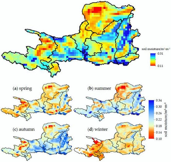
Figure 2.
Spatial distribution of annual average SM and seasonal SM in the YRB from 2000 to 2015.
SM was relatively low in most areas of the upper reaches of the basin, including the Inner Mongolia Autonomous Region, Northern Ningxia Autonomous Region, Western Gansu Province, Qinghai Province, and Sichuan Province; the lowest SM value occurred in the Northwest the Inner Mongolia Autonomous Region and the Northeast of Qinghai Province, but in individual places, such as Western Gansu Province and Central and Northern Qinghai Province, there were some high SM values, with a maximum value of up to 0.31 m3·m−3. SM was relatively high in most areas of the middle reaches of the basin, including Shanxi Province, Henan Province, Shaanxi Province, and Eastern Gansu Province, and the overall SM in Shanxi Province was relatively high, with a decreasing trend from northeast to southwest, while SM was relatively high in only a small part of other provinces. In general, the middle reaches of the basin as a whole showed a “funnel” decreasing trend.
From the seasonal distribution characteristics of SM, the SM in spring was relatively low, from 0.10 to 0.29 m3·m−3, and the regions with low values were the northeast and west of the upper reaches of the basin and the center of the middle reaches of the basin. In summer, the SM was relatively high, ranging from 0.10 to 0.34 m3·m−3, and the low value was mainly concentrated in the northeast of the upper reaches of the basin. In autumn, the SM in the basin was relatively high on the whole, ranging from 0.10 to 0.34 m3·m−3, with only very few low areas. The winter season is affected by seasonal snow and permafrost, resulting in some null values in the ESA CCI SM data. The overall SM of the basin was low, particularly in the west of the upper reaches, which was 0.10–0.25m3·m−3.
In order to further analyze the spatial dynamic change trend of the YRB in recent years, the spatial distribution of annual SM was analyzed for four specific times: 2000, 2005, 2010, and 2015. As can be seen from Figure 3, the spatial distribution of SM in the YRB was roughly the same in the four years, and the low values of SM all occurred in the Inner Mongolia Autonomous Region and northeastern Qinghai Province of the upper reaches of the YRB. The high values of SM were found in the north-central Shanxi Province, southwestern Henan Province, northeastern Shaanxi Province, and central Gansu Province. The only difference was that the SM in northwest Qinghai Province in the upper reaches of the basin in Figure 3b was relatively high, which may be due to the annual precipitation in the year 2005 of northwest Qinghai Province being approximately 620mm, much greater than 470 mm (the multi-year average). Therefore, the abundance of precipitation caused relatively high soil moisture in the area.
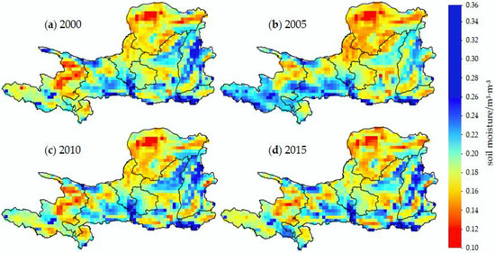
Figure 3.
Spatial distribution of annual SM in the YRB at four specific times.
In summary, although the spatial distribution of SM varied slightly over the years, it generally showed a decreasing trend from south to north, which is broadly consistent with the distribution law of SM shown in Figure 2. Therefore, it could be concluded that the spatial distribution of SM in the YRB over the last 16 years had a certain stability.
3.2. Temporal Variation of Soil Moisture
3.2.1. Interannual Variation
As can be seen from Figure 4, the interannual variation of SM from 2000 to 2015 showed an irregular “sawtooth” variation pattern, with an overall upward trend (~0.0005 m3·m−3·a−1) but not significant. The annual average SM in the YRB for the last 16 years was 0.19 m3·m−3, the lowest value of SM appeared in 2002 with a value of 0.18 m3·m−3, and the maximum value of 0.20 m3·m−3 occurred in 2014.
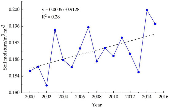
Figure 4.
Interannual variation of SM in the YRB from 2000 to 2015.
The annual average SM in the YRB from 2000 to 2015 was analyzed by M-K trend test methods, and the UF and UB curves for the M-K trend tests were plotted (Figure 5). As can be seen from Figure 5, the SM in the YRB showed an increased but non-significant trend from 2000 to the second half of 2001; from the second half of 2001 to the first half of 2002, the SM showed a non-significant downward trend, and from the second half of 2002 to 2015, the SM showed a non-significant upward trend. The annual average SM UF and UB curves had an intersection between 2005 and 2006, and the corresponding UF value was greater than 0 and less than 1.96, indicating that this time node was the abrupt change point of no significant increase in annual SM.
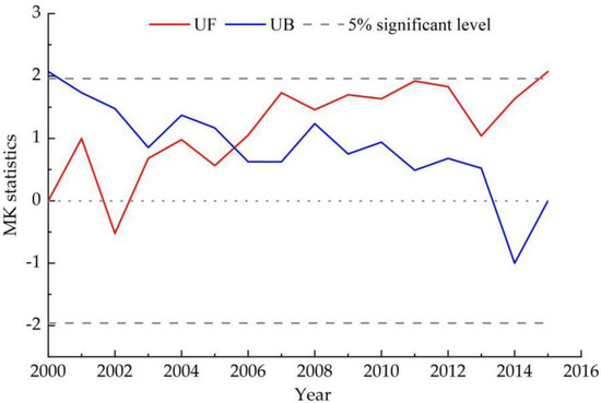
Figure 5.
The M-K statistics of annual average SM in the Yellow River Basin from 2000 to 2015.
Combined with Figure 4 and Figure 5, it could be concluded that although the variation of the SM in the YRB fluctuated up and down over these 16 years, its change amplitude is relatively small and showed a non-significant upward trend on the whole.
In this paper, by calculating the linear trend coefficient of SM, the change trend distribution of SM in the Yellow River Basin from 2000 to 2015 was obtained, as shown in Figure 6. As can be seen from the figure, in the past 16 years, most areas in the upper reaches of the YRB have shown an obvious wetting trend, with a value of 0.00047 m3·m−3·year−1, including central Inner Mongolia Autonomous Region, Ningxia Autonomous Region, central Gansu Province, Qinghai Province, and Sichuan Province. However, the annual average SM in these areas was relatively low. Most areas in the middle reaches of the YRB, such as Shanxi Province, Henan Province, central Shaanxi Province, and eastern Gansu Province, have shown an obvious drought trend, with a value of −0.00030 m3·m−3·year−1, yet the annual average SM in these areas was relatively high. Therefore, it could be concluded that the linear variation trend of SM in the YRB was roughly opposite to the spatial distribution trend of the annual average SM, especially in the east of the middle reaches of the basin. This is consistent with the research results of Yao et al. [20].
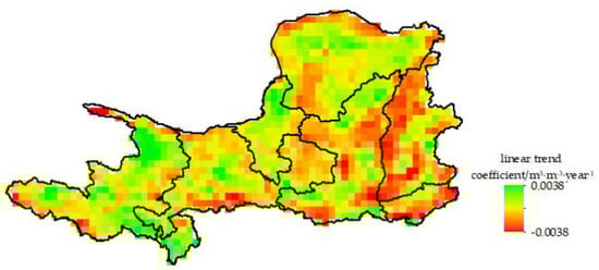
Figure 6.
Linear trend distribution of annual average SM in the YRB from 2000 to 2015.
3.2.2. Seasonal Variation
The multi-year monthly average SM curve over time in the YRB is shown in Figure 7. It could be seen that SM increased from the lowest value of 0.16 m3·m−3 from January until March; from March to April, SM decreased slightly, which may be caused by the increase in water demand for surface vegetation and the relatively low water storage in the early stage; from April to September, the SM entered a state of continuous increase, and reached the maximum value of 0.23 m3·m−3 in September; from September to December, the SM decreased continuously. The overall change trend of the multi-year monthly average SM over time showed an increase followed by a decrease.
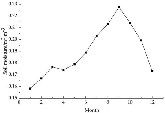
Figure 7.
Variation curve of monthly average SM in the Yellow River Basin from 2000 to 2015.
Figure 8 shows the seasonal variation of SM in the YRB from 2000 to 2015. As can be seen from the figure, the SM was highest in autumn, with relatively large variations in amplitude and an overall upward trend with a tendency rate of 0.0008 m3·m−3·a−1; followed by summer, with a relatively small variation amplitude and an overall upward trend with a tendency rate of 0.0014 m3·m−3·a−1; the next was spring, with the smallest variation amplitude and an overall upward trend with a tendency rate of 0.0007 m3·m−3·a−1; in winter, the SM was the lowest, and the amplitude of variation was the largest, with an overall downward trend with a tendency rate of −0.0007 m3·m−3·a−1. The SM in the YRB showed overall seasonal characteristics of autumn > summer > spring > winter.
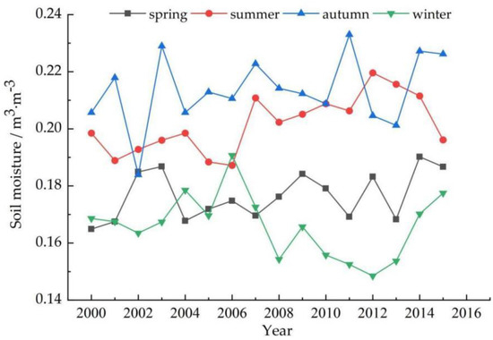
Figure 8.
The SM variation curve of the four seasons in the YRB from 2000 to 2015.
3.3. Analysis of Influencing Factors of Soil Moisture
3.3.1. Relationship between Soil Moisture and NDVI
Existing studies have shown that vegetation cover is one of the factors influencing the spatial-temporal variation of SM [38,39,40]. The surface vegetation can not only directly affect the hydrological process of the soil but also affects the change in SM through water absorption by plant roots and net rainfall. Vegetation affects SM mainly in the following ways: the leaf crown of vegetation can intercept rainfall, reduce evaporation consumption of SM, and enhance transpiration loss; covering the ground with dead leaves can increase SM infiltration, and the roots of vegetation can not only absorb SM but also promote the infiltration of surface water [41].
The seasonal changes of SM and NDVI are shown in Figure 9a; it can be seen that the overall variation trend of SM and NDVI was roughly the same, both showing a changing trend of increasing first and then decreasing. The variation time of SM lagged roughly 1 month behind NDVI.
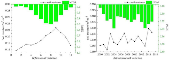
Figure 9.
Seasonal and interannual variation of SM and NDVI in the Yellow River Basin, 2000 to 2015.
In terms of interannual variation (Figure 9b), both NDVI and SM showed the trend of upward and downward fluctuations and had a certain correlation, but they were not very intuitive, so further analysis of their correlation is needed.
The results of the interannual correlation analysis of SM and NDVI are shown in Table 1. It can be seen that SM and NDVI showed significant positive correlations from 2000 to 2015. Among them, the year with the largest correlation coefficient was 2012, which reached 0.945 (p < 0.01); 2013 and 2010 followed, but also had significant correlations, the correlation coefficients were 0.942 and 0.910, respectively (p < 0.01); the lowest value occurred in 2006, 0.312; both of the other years also had better correlation.

Table 1.
Correlation analysis between SM and NDVI.
3.3.2. Relationship between Soil Moisture and Precipitation
Figure 10 shows the relationship between seasonal and interannual variations of SM and precipitation in the YRB from 2000 to 2015. As can be seen from Figure 10a, the seasonal variation trend of SM and precipitation was roughly the same, and as with NDVI, both showed a trend of increasing first and then decreasing; the slight decrease in SM from March to April may be caused by the low precipitation in the earlier period and the increased water demand of the surface vegetation during this time. The change time of SM lagged roughly 1 month behind precipitation.
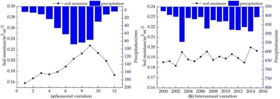
Figure 10.
Seasonal and interannual variation of SM and precipitation in the Yellow River Basin, 2000 to 2015.
The interannual variation relationship between them is shown in Figure 10b. It could be seen that the variation trend of annual average SM and annual precipitation was roughly the same; the annual average SM in years with high precipitation was relatively high, while the annual average SM in years with low precipitation was relatively low.
The results of the interannual correlation analysis of SM and precipitation are shown in Table 2. It can be seen that there was a significant positive correlation between SM and precipitation from 2000 to 2015. Among them, the correlation coefficient was the highest in 2013, which reached 0.867 (p < 0.01); the lowest value occurred in 2006, which was 0.149 (not significant); SM and precipitation also reached an extremely significant correlation (p < 0.01) in 2002, 2010, 2012, and 2014; and SM and precipitation in other years were also well correlated.
Table 2.
Correlation analysis between SM and precipitation.
3.3.3. Relationship between Soil Moisture and Air Temperature
Figure 11 shows the relationship between seasonal and interannual variations of SM and air temperature in the YRB from 2000 to 2015. As can be seen from Figure 11a, the seasonal variation trend of SM and the air temperature was roughly the same, both showing an increasing trend followed by a decreasing trend. Among them, the highest air temperature value of the year occurred in July, with a value of 18.12 ℃, and the maximum value of SM occurred in September, with a value of 0.23 m3·m−3; combined with the changing trend of the two curves in the figure, it could be concluded that the change time of SM was roughly 1–2 months behind the air temperature.

Figure 11.
Seasonal and interannual variation of SM and air temperature in the Yellow River Basin, 2000 to 2015.
The interannual variation is shown in Figure 11b; although both SM and air temperature curves showed a changing trend of up and down fluctuations, they were also correlated to some extent, so the correlation between them could be further analyzed.
The results of the interannual correlation analysis of SM and air temperature are shown in Table 3. It can be seen that SM and air temperature showed a positive correlation in general from 2000 to 2015, and a negative correlation was only found in 2006, with a low correlation of −0.027. In the past 16 years, the correlation coefficient was the largest in 2012, which reached 0.894 (p < 0.01); SM and air temperature also reached a highly significant correlation (p < 0.01) in 2002, 2010, 2012, and 2013, and SM and air temperature in other years were also well correlated.
Table 3.
Correlation analysis between SM and air temperature.
3.3.4. Relationship between Soil Moisture and Wind Speed
Wind speed affects the change in SM mainly by influencing evaporation from the soil and transpiration from the vegetation. Figure 12 shows the relationship between seasonal and interannual variations of SM and wind speed. It can be seen from Figure 12a that these two curves showed a “bimodal” variation trend. From January to March, the SM increased with the increase in wind speed, which may be because the soil was in the frozen period during this period; the SM was less affected by wind speed, mainly by precipitation, NDVI, and other factors; from April to December, the SM decreased (increased) with the increase (decrease) of wind speed, and the changing trend was just the opposite.
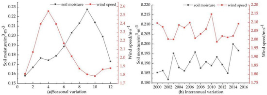
Figure 12.
Seasonal and interannual variation of SM and wind speed in the Yellow River Basin, 2000 to 2015.
In terms of interannual variation, it is clear from Figure 12b that the variation trends of SM and wind speed were quite different, and the correlation between the two was not strong.
The results of the interannual correlation analysis of SM and wind speed are shown in Table 4. It can be seen that SM and wind speed showed a negative correlation in general from 2000 to 2015, and a positive correlation was only found in 2002, with a low correlation of 0.177. In the past 16 years, the correlation coefficient was the largest in 2006, which was −0.822 (p < 0.01), followed by 2004; the SM and wind speed were also correlated in other years.
Table 4.
Correlation analysis between SM and air wind speed.
3.4. Analysis of Principal Factors
The KMO test was first carried out on these four environmental factors, and the result showed that the mean KMO value of these four environmental factors was 0.588 > 0.5, and the significance was less than 0.05, indicating that principal component analysis could be applied. The results of the principal component analysis are shown in Table 5. The cumulative contribution of principal component 1 and principal component 2 reached 95.74%; that is, these two principal components represented 95.74% of the four environmental factors. Therefore, the environmental factors affecting the spatial-temporal variation of SM in the YRB could be divided into two main components.
Table 5.
Contribution of principal components and cumulative variance.
The correlations between the two main components and the variables are shown in Table 6, and the load quantity represents the correlation coefficient between the principal component and each variable. It could be seen that principal component 1 had a high correlation with NDVI, precipitation, and air temperature at 0.973, 0.957, and 0.943, respectively, while principal component 2 had the highest correlation with wind speed at 0.995.
Table 6.
Initial factor load matrix.
Therefore, combined with the contribution rate of principal components 1 and 2 and the proportion of each variable in the principal component, the influence degree of these four environmental factors on SM in the YRB was determined as follows: NDVI > precipitation > air temperature > wind speed. However, the degree of influence of NDVI and precipitation on SM was not very different, so further comparative analysis of the correlation between the two and SM was needed.
Table 1 and Table 2 of Section 3.3 show the temporal correlation between NDVI and precipitation and SM. It can be seen that the correlation coefficient of NDVI was slightly greater than precipitation on the whole, especially in 2010, 2012, and 2013.
As can also be seen in Figure 13, the spatial distribution of precipitation, NDVI, and SM was roughly the same, all showing a decreasing trend from southeast to northwest.
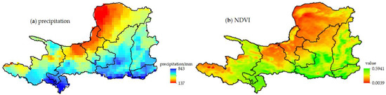
Figure 13.
Spatial distribution of annual mean precipitation and NDVI in the Yellow River basin from 2000–2015.
The spatial correlation between these two environmental factors and SM is shown in Figure 14. As can be seen in Figure 14a, precipitation and SM had an obvious positive correlation in the upper reaches of the basin; in the middle reaches of the basin, the correlation was low and negative in a few areas; the correlation coefficients ranged from −0.43 to 0.92, with an average of 0.52, indicating a significant positive correlation between the two on the whole.
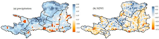
Figure 14.
Correlation between precipitation, NDVI, and SM from 2000 to 2015.
As can be seen from Figure 14b, the correlation coefficient between NDVI and SM ranged from −0.73 to 0.71, with an average value of 0.06; although the basin as a whole showed a positive correlation, it showed a negative correlation in the upper reaches western and middle reaches of the basin, this may be because there is too much vegetation in areas with high vegetation coverage, which leads to an increase in evapotranspiration and thus a decrease in SM.
In general, the spatial correlation between precipitation and SM was greater than that of NDVI.
Existing studies [42,43] show that the interannual variation of precipitation in the upper reaches of the basin shows a significant upward trend and the interannual variation of NDVI shows a slight upward trend; as can be seen in Figure 2 and Figure 14, in the upper reaches of the basin, although the annual mean value of SM is relatively low, it is positively correlated with precipitation and NDVI, and combined with the above studies, it can be concluded that the interannual variation of SM in the upper reaches of the basin shows a wet trend. Similarly, these studies also show that the interannual variation of NDVI shows a significant upward trend in the middle reaches of the basin as a whole, while the interannual variation of precipitation shows a non-significant upward trend, as can be seen in Figure 2 and Figure 14, in the middle reaches of the basin, the annual mean value of SM is relatively high, but show a significant negative correlation with NDVI, and a small positive correlation with precipitation and a negative correlation in individual areas. Combined with the above studies, it can be concluded that the interannual variation of SM in the upper reaches of the basin shows a dry trend. Taken together, this also explains the phenomenon that the linear variation trend of SM above is opposite to the spatial distribution trend of annual average SM (especially in the middle reaches of the basin).
In summary, through comparative analysis, it was determined that NDVI and precipitation were the main factors influencing the spatial-temporal variation of SM.
4. Conclusions
In this study, we used geostatistical methods to explore the spatial distribution characteristics of SM in the YRB, and the results showed that the annual average value of SM in the YRB is 0.11–0.31 m3·m−3. SM showed an overall decreasing trend from southeast to northwest, which is consistent with the climate distribution characteristics of the YRB, and the spatial distribution had a certain stability.
The annual average SM in the YRB had shown an overall upward trend over the last 16 years, but not significantly, with a tendency rate of 0.0005 m3·m−3·a−1. Through the M-K trend test methods analysis, it was concluded that 2005–2006 is the abrupt change point of soil moisture increase. In the past 16 years, the upper reaches of the YRB have shown a wet trend, with a value of 0.00047 m3·m−3·year−1; while the middle reaches have shown an obvious drought trend, especially in Shanxi Province and Henan Province, with a value of −0.00030 m3·m−3·year−1, drought research may become the focus of future research in these regions. SM in the YRB had exhibited the seasonal characteristics of autumn > summer > spring > winter, with a tendency rate of 0.0008, 0.0014, 0.0007, and −0.0007 m3·m−3·a−1, respectively.
The correlation analysis method was used to explore the relationships between SM and NDVI, precipitation, air temperature, and wind speed, respectively. The results showed that SM is positively correlated with NDVI, precipitation, and air temperature on the whole and negatively correlated with wind speed. Combined with PCA methods, NDVI and precipitation were determined as the main factors affecting the spatial-temporal variation of SM. It was found in the study that the influence of precipitation, temperature, and NDVI on SM has a certain lag time of roughly 1–2 months, which is not explained in this paper, and these analyses will be supplemented and improved in future work.
There may be some shortcomings in this study, such as the relatively low spatial resolution of ESA CCI soil moisture data and the serious loss of this data in winter; also, the influence of human activities are rarely taken into account in SM changes. Although there are some limitations in this study, it also presents some meaningful results on the spatial-temporal distribution characteristics and attributions of SM in the YRB in recent years. In view of this, future research should focus on multi-source data fusion technology and downscaling technology to make up for the lack of ESA CCI SM data and improve spatial resolution to improve the application value of this product in the field of SM research. At the same time, the comprehensive influence of environmental factors and human activities should be taken into account to further clarify the internal laws and causes of the spatial-temporal variation of SM so as to provide a scientific basis for the management of water resources in the basin.
Author Contributions
Conceptualization, L.G., B.Z. and H.J.; methodology, L.G. and B.Z.; software, L.G. and Y.Z.; validation, L.G., B.Z. and H.J.; formal analysis, L.G.; investigation, L.G.; resources, B.Z.; data curation, L.G., Y.M., H.S. and Y.H.; writing—original draft preparation, L.G.; writing—review and editing, L.G., B.Z. and H.J.; visualization, L.G. and B.Z.; supervision, B.Z. and H.J. All authors have read and agreed to the published version of the manuscript.
Funding
This research was funded by the Shanxi Province Water Conservancy Science and Technology Research and Promotion Project, Grant No.2022GM001 and Shanxi Province Basic Research Program for Young Scientists, Grant No. 202103021223078.
Institutional Review Board Statement
Not applicable.
Informed Consent Statement
Not applicable.
Data Availability Statement
The ESA CCI SM data used in this study are available from https://www.esa-soilmoisture-cci.org/ (accessed on 12 March 2022). The original meteorological data are provided by the National Meteorological Science Data Center (http://data.cma.cn/, (accessed on 20 October 2021)). The NDVI data used in this study come from the National Earth System Science Data Center (http://www.geodata.cn, (accessed on 15 March 2022)).
Acknowledgments
The authors acknowledge the European Space Agency, the National Meteorological Science Data Centerm and the National Earth System Science Data Center for providing the data, and thank the Editor-in-Chief Reka Kirmajer and the anonymous reviewers for their guidance on this article.
Conflicts of Interest
The authors declare no conflict of interest.
References
- Fuentes, I.; Padarian, J.; Vervoort, R.W. Towards near real-time national-scale soil water content monitoring using data fusion as a downscaling alternative. J. Hydrol. 2022, 609, 127705. [Google Scholar] [CrossRef]
- Tavakol, A.; McDonough, K.R.; Rahmani, V.; Hutchinson, J.M. The soil moisture data bank: The ground-based, model-based, and satellite-based soil moisture data. Remote Sens. Appl. Soc. Environ. 2021, 24, 100649. [Google Scholar] [CrossRef]
- He, X.T.; Yuan, S.J.; Pan, T.; Gu, X.P.; Yu, F. Spatial-temporal distribution characteristics of soil moisture in karst region of Guizhou Province. Carsologica Sin. 2018, 37, 562–574. [Google Scholar]
- Peng, J.; Jonathan, N.; Alexander, L.; Zhang, S.Q.; Wang, J. Evaluation of Satellite and Reanalysis Soil Moisture Products over Southwest China Using Ground-Based Measurements. Remote Sens. 2015, 7, 15729–15747. [Google Scholar] [CrossRef]
- Liu, Y.; Wang, W.; Liu, Y. ESA CCI Soil Moisture Assimilation in SWAT for Improved Hydrological Simulation in Upper Huai River Basin. Adv. Meteorol. 2018, 2018, 1–13. [Google Scholar] [CrossRef]
- Prashant, K.S. Satellite Soil Moisture: Review of Theory and Applications in Water Resources. Water Resour. Manag. 2017, 31, 3161–3176. [Google Scholar]
- Lou, D.; Wang, G.; Shan, C.; Hagan, D.F.T.; Ullah, W.; Shi, D. Changes of Soil Moisture from Multiple Sources during 1988–2010 in the Yellow River Basin, China. Adv. Meteorol. 2018, 2018, 1–14. [Google Scholar] [CrossRef]
- Acosta, J.A.; Gabarrón, M.; Martínez-Segura, M.; Martínez-Martínez, S.; Faz, A.; Pérez-Pastor, A.; Gómez-López, M.D.; Zornoza, R. Soil Water Content Prediction Using Electrical Resistivity Tomography (ERT) in Mediterranean Tree Orchard Soils. Sensors 2022, 22, 1365. [Google Scholar] [CrossRef]
- Baldocchi, D.D.; Keeney, N.; Rey-Sanchez, C.; Fisher, J.B. Atmospheric humidity deficits tell us how soil moisture deficits down-regulate ecosystem evaporation. Adv. Water Resour. 2022, 159, 104100. [Google Scholar] [CrossRef]
- Xie, P.Y.; Liu, Z.X. Research on the principle and technical method of soil moisture measurement. Mod. Agric. Sci. Technol. 2020, 23, 166–168. [Google Scholar]
- Kim, S.; Zhang, R.; Pham, H.; Sharma, A. A Review of Satellite-Derived Soil Moisture and Its Usage for Flood Estimation. Remote Sens. Earth Syst. Sci. 2019, 2, 225–246. [Google Scholar] [CrossRef]
- Yang, J.J.; Cai, H.J.; Wang, S.H.; Xie, H.X. Research on the relationship between shallow soil moisture and deep soil moisture in Yangling District. Agric. Res. Arid Areas 2010, 28, 53–57. [Google Scholar]
- Liu, S.X.; Xing, B.; Yuan, G.F.; Mo, X.G.; Lin, Z.H. Analysis of the relationship between rhizosphere and surface soil water in China. Chin. J. Plant Ecol. 2013, 37, 1–17. [Google Scholar] [CrossRef]
- Li, Y.; Liu, D.; Li, T.; Fu, Q.; Liu, D.; Hou, R.; Meng, F.; Li, M.; Li, Q. Responses of spring soil moisture of different land use types to snow cover in Northeast China under climate change background. J. Hydrol. 2022, 608, 127610. [Google Scholar] [CrossRef]
- Ali, G.A.; Roy, A.G.; Legendre, P. Spatial relationships between soil moisture patterns and topographic variables at multiple scales in a humid temperate forested catchment. Water Resour. Res. 2010, 46, 2290–2296. [Google Scholar] [CrossRef]
- Miyamoto, T.; Putiso, M.; Shiono, T.; Taruya, H.; Chikushi, J. Spatial and Temporal Distribution of Soil Water Content in Fields under Different Vegetation Conditions Based on TDR Measurements. Jpn. Agric. Res. Q. 2014, 37, 243–248. [Google Scholar] [CrossRef][Green Version]
- Fan, K.K.; Zhang, Q.; Sun, P.; Song, C.Q.; Zhu, X.D.; Yu, H.Q.; Shen, Z.X. The surface soil water changes, influence factors and future estimates of the Qinghai-Tibet Plateau. Acta Geogr. Sin. 2019, 74, 520–533. [Google Scholar]
- Getachew, A.; Tsegaye, T.; Berhan, G. Monitoring Residual Soil Moisture and Its Association to the Long-Term Variability of Rainfall over the Upper Blue Nile Basin in Ethiopia. Remote Sens. 2020, 12, 2138. [Google Scholar]
- Gao, K.; Gai, A.H.; Pan, T.; Ma, Z.A.; Lu, X. Spatial variability of soil moisture and its main control factors in the Yellow River source area. J. Gansu Agric. Univ. 2019, 54, 166–174. [Google Scholar]
- Yao, X.L.; Jiang, Q.; Liu, Y.; Li, L.Y.; Wang, Q.Y.; Yu, J.S. Spatiotemporal variation of soil moisture in Northern China based on climate change initiative data. Agron. J. 2021, 113, 774–785. [Google Scholar] [CrossRef]
- Wang, Y.; Cao, J.; Liu, Y.; Zhu, Y.; Fang, X.; Huang, Q.; Chen, J. Spatiotemporal Analysis of Soil Moisture Variation in the Jiangsu Water Supply Area of the South-to-North Water Diversion Using ESA CCI Data. Remote Sens. 2022, 14, 256. [Google Scholar] [CrossRef]
- Liu, Y.; Zhu, Q.; Liao, K.; Lai, X.; Wang, J. Downscaling of ESA CCI soil moisture in Taihu Lake Basin: Are wetness conditions and non-linearity important. J. Water Clim. Chang. 2020, 12, 1564–1579. [Google Scholar] [CrossRef]
- Muhammad, Z.; Minha, C. Satellite-based global-scale irrigation water use and its contemporary trends. Sci. Total Environ. 2020, 714, 136719. [Google Scholar]
- de Figueiredo, T.; Royer, A.C.; Fonseca, F.; de Araújo Schütz, F.C.; Hernández, Z. Regression Models for Soil Water Storage Estimation Using the ESA CCI Satellite Soil Moisture Product: A Case Study in Northeast Portugal. Water 2020, 13, 37. [Google Scholar] [CrossRef]
- Hu, D.; Sha, S.; Wang, L.J.; Wang, W. Application of ESA active-passive microwave soil moisture fusion products in drought monitoring in Gansu Province. J. Arid Meteorol. 2019, 37, 517–528. [Google Scholar]
- Yao, X.L.; Yu, J.S.; Li, Z.J.; Song, H. Accuracy assessment of CCI remote sensing soil water in characterizing drought in the main grain producing areas of Northeast China. J. Beijing Norm. Univ. 2019, 55, 233–239. [Google Scholar]
- Dorigo, W.A.; Gruber, A.; De Jeu, R.A.M.; Wagner, W.; Stacke, T.; Loew, A.; Albergel, C.; Brocca, L.; Chung, D.; Parinussa, R.M.; et al. Evaluation of the ESA CCI soil moisture product using ground-based observations. Remote Sens. Environ. 2015, 162, 380–395. [Google Scholar] [CrossRef]
- Xu, X.Y.; Frey, S. Validation of SMOS, SMAP, and ESA CCI Soil Moisture Over a Humid Region. IEEE J. Sel. Top. Appl. Earth Obs. Remote Sens. 2021, 14, 10784–10793. [Google Scholar] [CrossRef]
- Ling, X.; Huang, Y.; Guo, W.; Wang, Y.; Chen, C.; Qiu, B.; Ge, J.; Qin, K.; Xue, Y.; Peng, J. Comprehensive evaluation of satellite-based and reanalysis soil moisture products using in situ observations over China. Hydrol. Earth Syst. Sci. 2021, 25, 4209–4229. [Google Scholar] [CrossRef]
- He, Z.; He, J.P. Remote sensing monitoring of spatial and temporal evolution of vegetation cover in the Yellow River basin in the past 32 years. Trans. Chin. Soc. Agric. Mach. 2017, 48, 179–185. [Google Scholar]
- Zhao, P.P.; Shao, M.G. Soil water spatial distribution in dam farmland on the Loess Plateau, China. Acta Agric. Scand. Sect. B-Plant Soil Sci. 2010, 60, 117–125. [Google Scholar] [CrossRef]
- Wang, J.; Fu, B.; Qiu, Y.; Chen, L.; Wang, Z. Geostatistical analysis of soil moisture variability on Da Nangou catchment of the loess plateau, China. Environ. Geol. 2001, 41, 113–120. [Google Scholar] [CrossRef]
- Tong, R.; Yang, X.; Ren, L.; Shen, H.; Shan, H.; Kong, H.; Lin, C. Spatio-temporal variation of surface soil moisture over the Yellow River basin during 1961–2012. Proc. Int. Assoc. Hydrol. Sci. 2015, 368, 391–396. [Google Scholar] [CrossRef][Green Version]
- Guo, M.; Li, J.; He, H.; Xu, J.; Jin, Y. Detecting Global Vegetation Changes Using Mann-Kendal (MK) Trend Test for 1982–2015 Time Period. Chin. Geogr. Sci. 2018, 28, 907–919. [Google Scholar] [CrossRef]
- Qiu, Y.; Fu, B.; Wang, J.; Chen, L.; Meng, Q.; Zhang, Y. Spatial prediction of soil moisture content using multiple-linear regressions in a gully catchment of the Loess Plateau, China. J. Arid Environ. 2009, 74, 208–220. [Google Scholar] [CrossRef]
- Chen, X.H. Study on the Mechanism of the Influence of Soil Water Content on Cold Resistance of Thermophilic Crops Based on Principal Component Analysis. IOP Conf. Ser. Earth Environ. Sci. 2021, 784, 012040. [Google Scholar] [CrossRef]
- Cui, J.X. The Space-Time Distribution of Soil Water and Temperature of a Desert Ecosystem Using Spatio-Temporal Kriging and PCA Analysis. J. Indian Soc. Remote Sens. 2020, 48, 271–286. [Google Scholar] [CrossRef]
- Maurya, A.K.; Murugan, D.; Singh, D. An approach for soil moisture estimation using urban and vegetation fraction cover from coarse resolution Scatsat-1 data. Adv. Space Res. 2021, 68, 1329–1340. [Google Scholar] [CrossRef]
- Wang, S.; Fu, B.J.; Gao, G.Y.; Yao, X.L.; Zhou, J. Soil moisture and evapotranspiration of different land cover types in the Loess Plateau, China. Hydrol. Earth Syst. Sci. 2012, 16, 2883–2892. [Google Scholar] [CrossRef]
- Qiu, L.; Wu, Y.; Wang, L.; Lei, X.; Liao, W.; Hui, Y.; Meng, X. Spatiotemporal response of the water cycle to land use conversions in a typical hilly–gully basin on the Loess Plateau, China. Hydrol. Earth Syst. Sci. 2017, 21, 6485–6499. [Google Scholar] [CrossRef]
- Zhao, C.; Zhang, L.H.; Li, J.L.; Tian, J.; Wu, W.Z.; Jin, X.; Zhang, X.F.; Jiang, Y.W.; Wang, X.L.; He, C.S.; et al. The relationship between spatial distribution of soil water content and environmental factors in the upper reaches of Heihe River. J. Lanzhou Univ. 2014, 50, 338–347. [Google Scholar]
- Zhang, Y.L.; Su, H.M.; Zhang, X.Y. Temporal and spatial analysis of vegetation cover change in the Yellow River Basin from 1998 to 2012. J. Desert Res. 2014, 34, 597–602. [Google Scholar]
- Wang, C.H.; Yang, J.T.; Yang, K.; Zhang, F.M.; Zhang, S.N.; Li, K.C.; Yang, Y. Temporal and spatial variation characteristics of precipitation over the Yellow River Basin in the past 60 years and its trend in the future 30 years. Arid Zone Res. 2022, 39, 708–722. [Google Scholar]


Publisher’s Note: MDPI stays neutral with regard to jurisdictional claims in published maps and institutional affiliations. |
© 2022 by the authors. Licensee MDPI, Basel, Switzerland. This article is an open access article distributed under the terms and conditions of the Creative Commons Attribution (CC BY) license (https://creativecommons.org/licenses/by/4.0/).