Article

Prediction Model for Daily Reference Crop Evapotranspiration Based on Hybrid Algorithm in Semi-Arid Regions of China

1
College of Agricultural Equipment Engineering, Henan University of Science and Technology, Luoyang 471000, China
2
College of International Education, Bohai University, Jinzhou 121013, China
3
Key Laboratory for Agricultural Soil and Water Engineering in Arid Area of Ministry of Education, Northwest A&F University, Xianyang 712100, China
4
Foundation Department, Liaoning Agriculture and Economy School, Jinzhou 121007, China
5
College of Mechanical and Electronic Engineering, Wuhan University of Technology, Wuhan 430070, China
*
Author to whom correspondence should be addressed.
Atmosphere 2022, 13(6), 922; https://doi.org/10.3390/atmos13060922
Submission received: 27 April 2022 / Revised: 20 May 2022 / Accepted: 2 June 2022 / Published: 6 June 2022
(This article belongs to the Section Atmospheric Techniques, Instruments, and Modeling)

Abstract

:
The accurate estimation of reference crop evapotranspiration (ETO) plays an important role in guiding regional water resource management and crop water content research. In order to improve the accuracy of ETO prediction in regions with missing data, this study used the partial correlation analysis method to select factors that have a large impact on ETO as input combinations to construct ETO estimation models for typical stations in semi-arid regions of China. A biological heuristic optimization algorithm (Golden Eagle optimization algorithm (GEO) and Sparrow optimization algorithm (SSA)) and Extreme Learning Machine model (ELM) were combined to improve the estimation accuracy. The results showed that Ra was the primary factor affecting the ETO model, with an importance range of 0.187–0.566. Compared with the independent ELM model, the hybrid model has higher accuracy and stability. The estimated value of the SSA-ELM model under five-factor input condition (Ra, RH, Tmax, Tmin, U2) is closest to the standard value calculated by FAO56 PM: RMSE = 0.067–0.085, R2 = 0.998–0.999, MAE = 0.050–0.066 and NSE = 0.998–0.999. In general, the combination of a partial correlation analysis algorithm and a hybrid model can be used to estimate ETO with high accuracy under the condition of reducing input factors. Use of the first five factors extracted from the partial correlation analysis algorithm as input to build an ETO estimation model based on SSA-ELM in China’s semi-arid regions is recommended, which can also provide a reference for ETO estimation in similar regions.

1. Introduction

Reference crop evapotranspiration (ETO) is an important parameter in the atmospheric cycle, which is related to agricultural management of water resources and earth energy balance [1]. About 60% of water enters the atmosphere through actual evapotranspiration (ETa) [2]. However, due to the difficulty of accurate determination of ETa, potential evapotranspiration (ETP)and ETO are often used to calculate agricultural water demand [3]. ETP is the upper limit of evapotranspiration under ideal crop irrigation conditions. ETO considers the growth of crops based on ETP. ETO defines the parameters of reference crops and can more easily estimate the evaporation of crops and vegetation surface, which is the essential factor in calculating the water budget. Therefore, the accurate estimation of ETO is of great significance in studying the water cycle between crops and the atmosphere. The annual and interannual distribution of precipitation in semi-arid areas of China is uneven, and drought often occurs in some areas, which has greatly affected the agricultural development of this area. Therefore, determining a reasonable and accurate ETO estimation method has important guiding significance for developing water-saving agriculture in semi-arid areas of China. The Penman–Monteith equation (PM) is a widely used ETO standard calculation method, which is recommended by FAO [4]. Some scholars have found that combining meteorological data and the FAO-56 PM to estimate ETO in semi-arid regions can obtain reliable results [5]. L’opez-Urrea et al. found that PM performed well in the Albacete region, which indicated that this method could be adapted to different regions [6]. However, the accuracy of FAO-56 PM depends on a variety of meteorological data, making it very difficult to obtain ETO in areas with missing meteorological data.
In recent years, ETO calculation methods based on a small amount of input data have been widely developed. The ETO estimation models available in the literature may be broadly classified as (1) fully physically-based combination models that account for mass and energy conservation principles; (2) semi-physically based models that deal with either mass or energy conservation; and (3) black-box models based on artificial neural networks, empirical relationships, and fuzzy and genetic algorithms [7,8]. Physical or semi-physical based empirical models include the 48-PM model (based on comprehensive method) [9,10], Blaney–Criddle, Hargreaves, and other models (based on temperature method) [11,12,13,14] and Makkink, Priestley–Taylor, Irmak, and other models (based on radiation method) [15,16,17,18]. However, the estimation accuracy of empirical models is low. For example, Akpootu et al. used six empirical models to estimate ETO in Nigeria [19], and the accuracy of the model was not satisfactory (RMSE greater than 1.2147). Valiantzas et al. [20] compared the simplified Penman formula based on temperature and humidity with the Hargreaves–Samani formula and other formulas. The accuracy when estimating ETO with this new simplified formula was 46% higher than that obtained using the Hargreaves–Samani formula, but the recommended method has poor adaptability in some sites (Seeley, Hastings, and Avalon). In sum, the applicability of the ETO model based on empirical formula is very different in different regions, and its popularization and application are difficult.
Due to the advantages of a machine learning algorithm in dealing with nonlinear problems, some scholars use the machine learning algorithm to establish a black-box model in ETO estimating, such as the support vector machine algorithm based on the kernel, random forest algorithm (RF) and Catboost algorithm based on trees, and the BP and limit learning machine (ELM) based on artificial neural networks [21]. An extreme learning machine (ELM) is a single hidden layer feed-forward neural network algorithm. The model established by it has the advantages of fewer input parameters, strong generalization ability, and fast running speed. It has great advantages in machine learning algorithms. For example, in previous studies, Fan et al. used a variety of machine learning algorithms (SVM, ELM, GBDT, etc.) to build ETO estimation models. It was found that the ELM model was superior to those of the regression models [22]. So, this study uses the more advantageous ELM algorithm to build the ETO model. Although the ETO model constructed by the machine learning algorithm has higher accuracy than the empirical model, it still has great development potential. Hyperparameters in machine learning models generally struggle to achieve optimization.
In order to improve the estimation ability of the model, some scholars use optimization algorithms to optimize the hyperparameters of the model. Wu et al. [23] used artificial bee colony (ABC), differential evolution (DE), and particle swarm optimization (PSO) algorithms to globally correct the Hargreaves model to estimate ETO in Southwest China. Compared with the four empirical models, PSO-HG was found to have the highest prediction accuracy and was most suitable for ETO estimation in Southwest China. Mohammadi et al. [24] coupled support vector regression (SVR) with a whale optimization algorithm (WOA) and applied this to the daily ETO modeling of three meteorological stations in Iran. Compared with the pure SVR model, SVR-WOA was found to have a higher estimation accuracy and better performance. Lu et al. [25] combined the mixed extreme gradient enhancement (XGBoost) model with the gray wolf optimizer (GWO) to predict the ETO in the first 1–3 months of subtropical China and compared this with XGB, multilayer perceptron (MLP) and M5 model tree (M5) model. The GWO-XGB model outperformed the other three models in spring, autumn and winter. In sum, based on the ELM algorithm, using the optimization algorithm to optimize the hyperparameters can obtain an estimation model with better applicability.
The type and number of input parameters have a great impact on the accuracy of a machine learning model. For example, Hatice et al. compared the accuracy of the ETO model under different inputs. The results showed that solar radiation is the most influential factor on the model [26]. A reasonable selection for model input is very important for the construction of an ETO model in data-deficient areas, and many studies lack a theoretical basis for the selection of model input factors [27,28,29]. The partial correlation analysis (PCA) method can be used to analyze the influence of different parameters. In this study, the PCA algorithm will be used to calculate the correlation between meteorological parameters and ETO. In this study, the combination of the PCA algorithm and machine learning model is used to construct ETO simplified model in China’s semi-arid areas and provide references for regions in similar climatic conditions. The research purposes are: (1) to select as few determinations as possible among the many meteorological factors for ETO estimation through partial correlation analysis; (2) to construct the simplified ETO model based on different hybrid optimization algorithms; (3) to evaluate the applicability of the ETO-simplified model for typical stations in semi-arid areas of China.

2. Materials and Methods

2.1. Data Sources

China’s semi-arid regions are mainly distributed in the Middle East of the temperate Inner Mongolia Autonomous Region, the warm temperate Jinshangan region (Shanxi, Shaanxi, and Eastern Gansu), the Qilian Mountains Qinghai Lake region, and the southern Tibet Autonomous Region in the plateau climate region. The precipitation in semi-arid areas is generally 200~400 mm, the vegetation in this area is sparse, and the evaporation is much higher than the rainfall. Due to the uneven distribution of precipitation within and between years, drought is more frequent; this has greatly affected crop yield in areas with a short growth period.
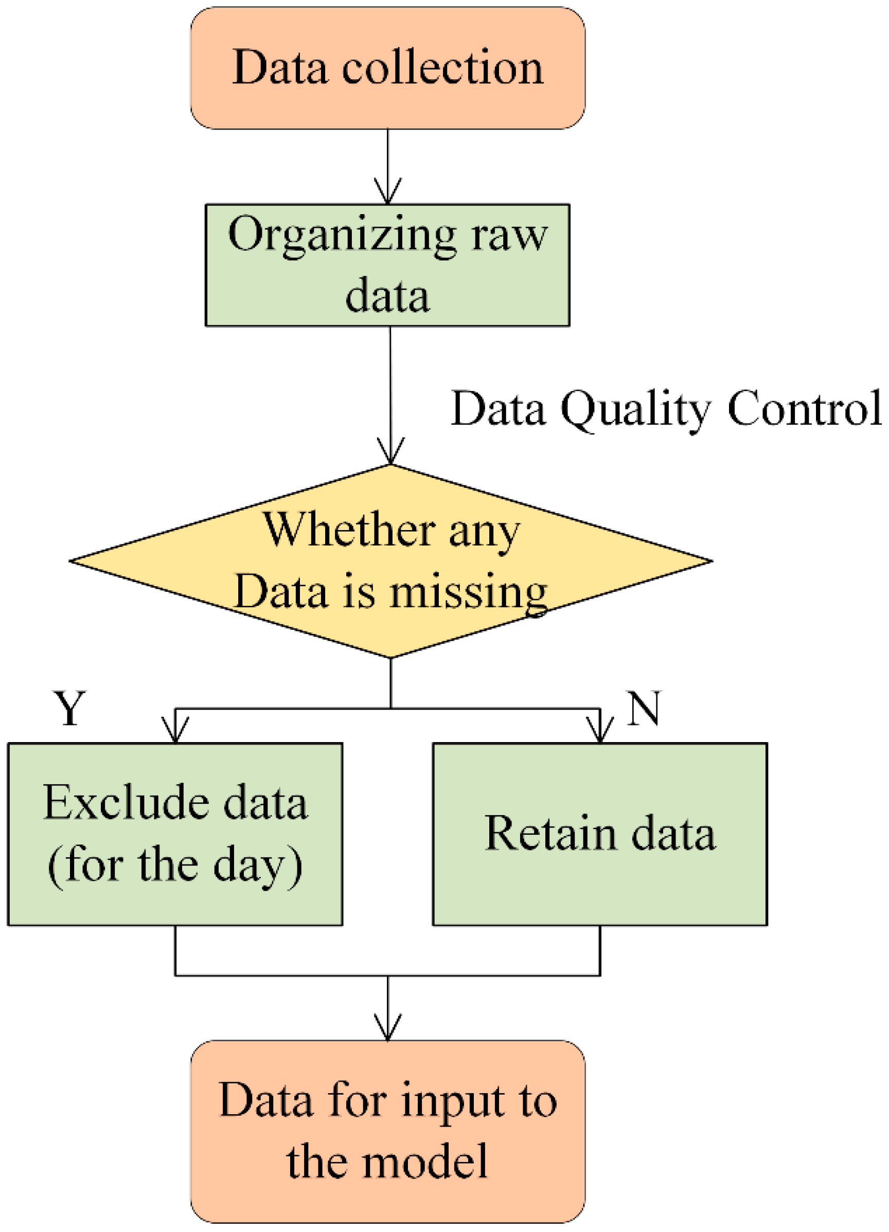
The data on meteorological stations in this study are from the China Meteorological data network (http://data.cma.cn/, accessed on 1 March 2021). This paper selected the daily meteorological data of seven typical stations in semi-arid areas (Bayinbuluke [51542], Dabancheng [51477], Xining [52866], Linxia [52984], Hequ [53564], Xilinhaote [54102], Dingri [55664]) from 1960 to 2019, including the maximum and minimum temperature (Tmax and Tmin), relative humidity (RH), solar radiation (Ra) and wind speed (U2). The map with elevation information is shown in Figure 1a. The map with LULC information is shown in Figure 1b. The flowchart of the preprocessing of raw datasets is shown in Figure 2. The division of the dataset refers to the previous research [30], in which 70% of the data were used as the training model, and 30% of the data were used to test the accuracy of the model. Table 1 shows the geographical locations and mean daily values of the meteorological data in this study.

2.2. FAO-56 PM

The daily reference evapotranspiration was calculated using the FAO-56 PM equation [31]:
E T 0 = 0.408 Δ ( R n G ) + γ 900 T m e a n + 273 U 2 ( e s e a ) Δ + γ ( 1 + 0.34 U 2 )
where Δ is saturated water pressure, slope of the temperature curve (kPa/°C), R n is the solar radiation of surface net (MJ m−2 day−1), G is the soil heat flux density (MJ m−2 day−1), and γ is the psychrometric constant (kPa °C−1). T m e a n is the mean air temperature (°C), U 2 is the wind speed at 2 m (M/s), e s is saturated vapor pressure (kPa), and e a is the actual vapor pressure (kPa).

2.3. Partial Correlation Analysis

Partial correlation analysis was used to analyze the correlation degree of two variables under the influence of multiple variables [32]. The Pearson correlation coefficient was the main index used to measure the direct correlation of variables. The Pearson correlation coefficient (PCCs) was used to calculate the correlation coefficient between variables without the influence of other variables, and understand the Pearson correlation coefficient from the perspective of the covariance matrix:
Assuming that there were two datasets, X and Y, and each contained n elements, the method of calculating their covariance is as follows:
C o v ( X , Y ) = i = 1 n ( x i E ( X ) ) ( y i E ( Y ) ) n
E(x) and E(y) represent their expectations, respectively. When x is greater than the average value of X and Y is greater than the average value of Y, the molecule is positive. When both are less than the average value, the molecule is also positive. However, if the two are not greater than or less than the average value at the same time, the molecule is negative. If the data are complex and the positive and negative offsets, the covariance will be relatively small, making it impossible to compare the correlation between the two. If the whole covariance has a relatively large positive or negative value, a correlation comparison can be carried out. If both are dimensional data, the dimension can be eliminated to obtain a dimensionless quantity (PCCs), and the normalization formula for eliminating the dimension is as follows:
ρ X , Y = C o v ( X , Y ) σ X σ Y = i = 1 n ( x i E ( X ) ) ( y i E ( Y ) ) i = 1 n ( x i E ( X ) ) 2 i = 1 n ( y i E ( Y ) ) 2

2.4. Development of Two Bionic Optimization Algorithms to Optimize ELM

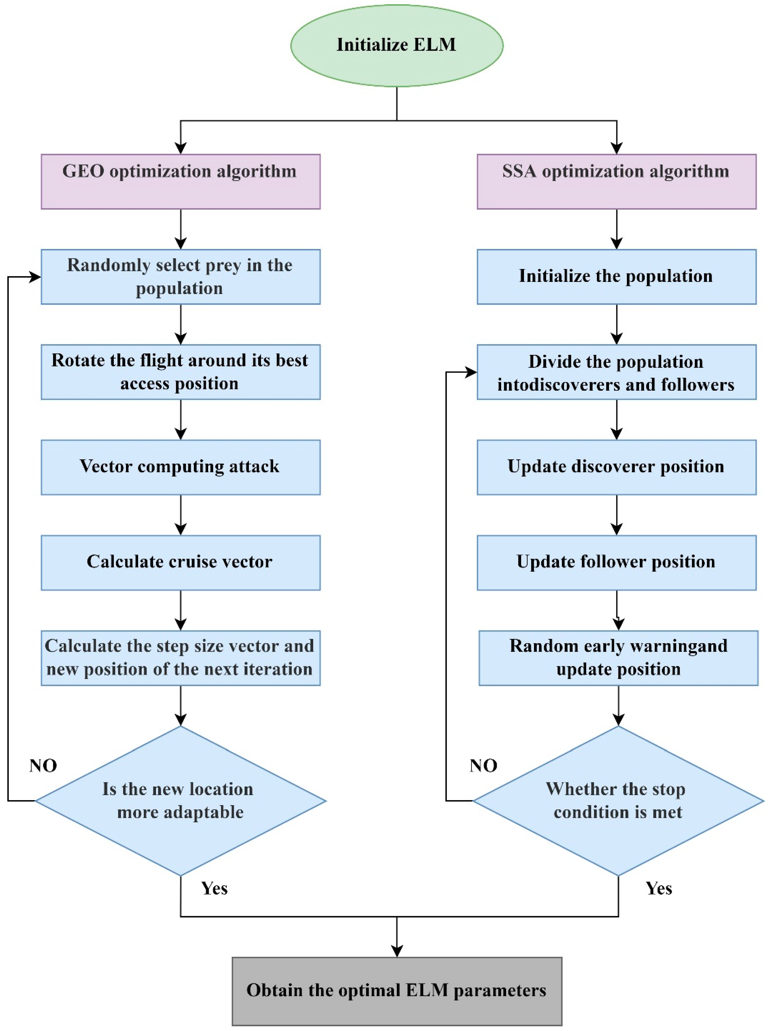
In this study, ELM, GEO-ELM, and SSA-ELM were established to estimate ETO. The initial threshold and weight of ELM are random, affecting the accuracy of the estimation model. To avoid the blind training of the ELM model, GEO and SSA algorithms are used to optimize the input weight and threshold of ELM. Then, the optimal weight threshold is assigned to ELM to establish the optimal ELM model. Figure 3 shows the construction process of the ETO model in this study.

2.4.1. ELM

ELM is a new, fast-learning algorithm [33]. For single hidden-layer neural networks, ELM can randomly initialize the input weight and bias and obtain the corresponding output weight. Suppose there are N arbitrary samples ( X i , t i ) , where X i = [ x i 1 , x i 2 , , x i n ] T R n , t i = [ t i 1 , t i 2 , , t i m ] T R m . For a single hidden layer neural network with L hidden layer nodes, this is expressed as:
i = 1 L β i g ( W i X j + b i ) = o j , j = 1 , , N
where g(x) is the activation function, W i = [ w i , 1 , w i , 2 , , w i , n ] T is the input weight, β i is the output weight, b i is the offset of the ith hidden layer unit, and oj is the output of the network for the sample xj, j = 1, ⋯, N.
The goal of single hidden layer neural network learning is to minimize the output error, which can be expressed as the following formula:
j = 1 N o j t j = 0
t_j is the output vector. Namely, β i , b i , and W i , make:
i = 1 L β i g ( W i X j + b i ) = t j , j = 1 , , N
The above equation can be written compactly as:
H β = T
H ( w 1 , , w N ˜ , b 1 , , b N ˜ , x 1 , , x N ) = [ g ( w 1 x 1 + b 1 ) g ( w N ˜ x 1 + b N ˜ ) g ( w 1 x N + b 1 ) g ( w N ˜ x N + b N ˜ ) ] N × N ˜
β is the output weights between hidden layer and output layer, where the i th row vector of β is β i = [ β i 1 , β i 2 , , β i m ] T which can be written in matrix form as:
β = [ β 1 T β 2 T β L T ] L × n = [ β 11 β 12 β 1 m β 21 β 22 β 2 m β L 1 β L 2 β L m ]
Therefore,
T = [ t 1 T t 2 T t N T ] N × m = [ t 11 t 12 t 1 m t 21 t 22 t 2 m t N 1 t N 2 t N m ]
H is called the hidden layer output matrix of the neural network; the i th column of H is the i th hidden node output with respect to inputs x 1 , x 2 , , x N .
To train single hidden-layer neural networks, we hope to obtain W ^ i , b ^ i , and β ^ i , and make:
H ( W ^ i , b ^ i ) β ^ i T = m i n W , b , β H ( W i , b i ) β i T
where i = 1 , , L , which is equivalent to minimizing the loss function:
E = j = 1 N ( i = 1 L β i g ( W i X j + b i ) t j ) 2

2.4.2. GEO

GEO is an optimization algorithm based on the spiral motion of golden eagles [34]. In the early stage of hunting, golden eagles show a greater tendency to patrol and look for prey. In the later stage of hunting, they show more tendency to attack to capture the best prey in the shortest time.
From the current position of the golden eagle to the position of the prey in the Golden Eagle’s memory, the attack vector of the Golden Eagle can be calculated according to the following formula:
A i = X f X i
A i is the attack vector of the ith Golden Eagle, X f is the best place (prey) reached by the golden eagle, and X i is the current position of the ith golden eagle.
The cruise vector of the golden eagle is calculated according to the attack vector, and the cruise can also be considered the linear speed of the Golden Eagle relative to its prey. The expression of Golden Eagle cruise vector in the next iteration is
j = 1 n a j x j = j = 1 n a j t x j
where A = [ a 1 , a 2 , , a n ] is the attack vector, X = [ x 1 , x 2 , , x n ] is the decision vector, and X = [ x 1 , x 2 , , x n ] is the position of the selected prey.
The displacement of the Golden Eagle is composed of attack and step vectors. The step vector of the Golden Eagle iteration is the following two formulas:
Δ x i = r 1 p a A i A i + r 2 p c C i C i
A i = j n a j 2 , C i = j n c j 2
where p a is the attack coefficient, p c is the cruise coefficient, and r 1 and r 2 are random vectors between [ 0 , 1 ] . If the Golden Eagle’s new location is more adaptable than its memory location, the eagle’s memory will be updated with the new location. The latest position of the Golden Eagle in this iteration is as follows:
x t + 1 = x t + Δ x i t
where x t + 1 is the position of the Golden Eagle’s t + 1st time, and x t is the position of the Golden Eagle’s t-th time; Δ x i t is the step size of the Golden Eagle’s movement.

2.4.3. SSA

The mathematical model of SSA is established with six main rules. The algorithm flow is created based on these six rules [35]. First, the population, the number of iterations, and the predator and the joiner ratios must be initialized; then, the fitness values can be calculated and ranked. In the simulation experiments of the Sparrow Search Algorithm, virtual sparrows must be used to find food, and the population, consisting of only sparrows, can be represented in the following form:
X = [ x 1 1 x 1 2 x 1 d x 2 1 x 2 2 x 2 d x n 1 x n 2 x n d ]
where d is the number of dimensions indicating the variables of the problem to be optimized and n is the number of sparrows. Then, the fitness values of all sparrows can be expressed in the following form:
F x = [ f ( [ x 1 1 x 1 2 x 1 d ] ) f ( [ x 2 1 x 2 2 x 2 d ] ) f ( [ x n 1 x n 2 x n d ] ) ]
where f denotes the fitness value.
Then, the predator position is updated, the joiner position is updated, the alert position is updated, the fitness value is calculated, and the sparrow position is updated. The optimization of the ELM algorithm requires that the SSA algorithm is optimized for both its regularization coefficient C and kernel function parameter S . The fitness function is designed as the MSE of the error of the training set:
fitness = argmin ( MSE pridect )
The MSE error after training is chosen as the fitness function. The smaller the MSE error, the better the predicted data overlap with the original data. The final optimized output is the optimal regularization coefficient C and kernel function parameter S . The trained network is then tested on the test dataset using the optimal regularization coefficient C and kernel function parameter S .

2.5. Model Prediction Evaluation

The root mean squared error (RMSE), coefficient of determination (R2), Nash–Sutcliffe efficiency coefficient (NSE), mean absolute error (MAE), and GPI were used to evaluate the performance of the ETO model [36].
RMSE = 1 n i = 1 n ( g i h i ) 2
R 2 = [ i = 1 n ( g i g ¯ ) ( h i h ¯ ) ] 2 i = 1 n ( g i g ¯ ) 2 i = 1 n ( h i h ¯ ) 2
MAE = 1 n i = 1 n | g i h i |
NSE = 1 i = 1 n ( g i h i ) 2 i = 1 n ( h i h ¯ ) 2
GPI = j = 1 4 α j ( T j T ¯ j )
where g i and h i are the simulated and measured values, respectively; n is the number of measured values; g ¯ and h ¯ are the means of the simulated and measured values, respectively. T j is the normalised value of RMSE, MAE, R2, and NSE, and T ¯ j is the median of the corresponding parameter; when T j is RMSE and MAE, α j is −1 or 1 otherwise.

3. Results and Discussion

3.1. Selecting Important Weather Factors with Partial Correlation Analysis

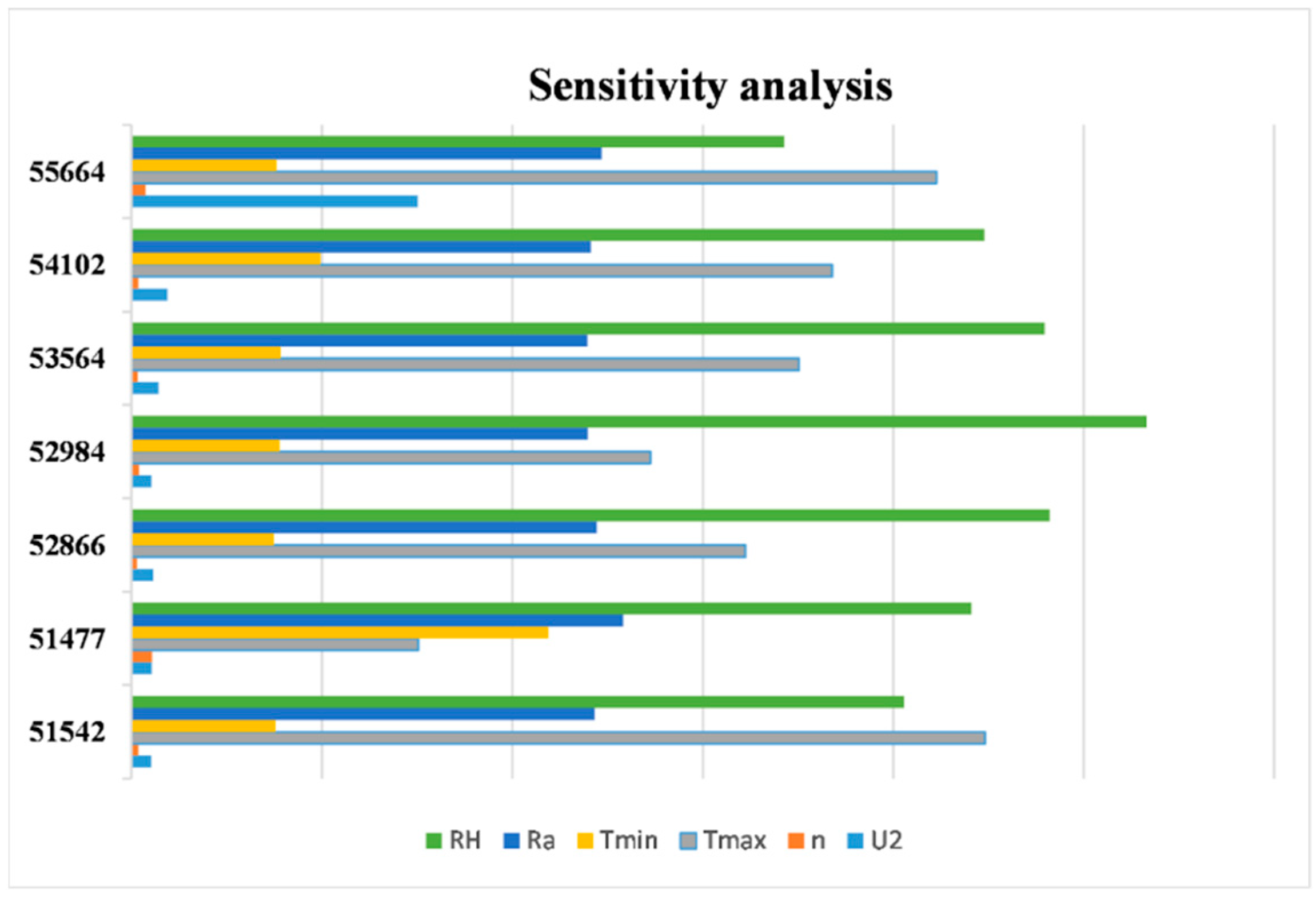
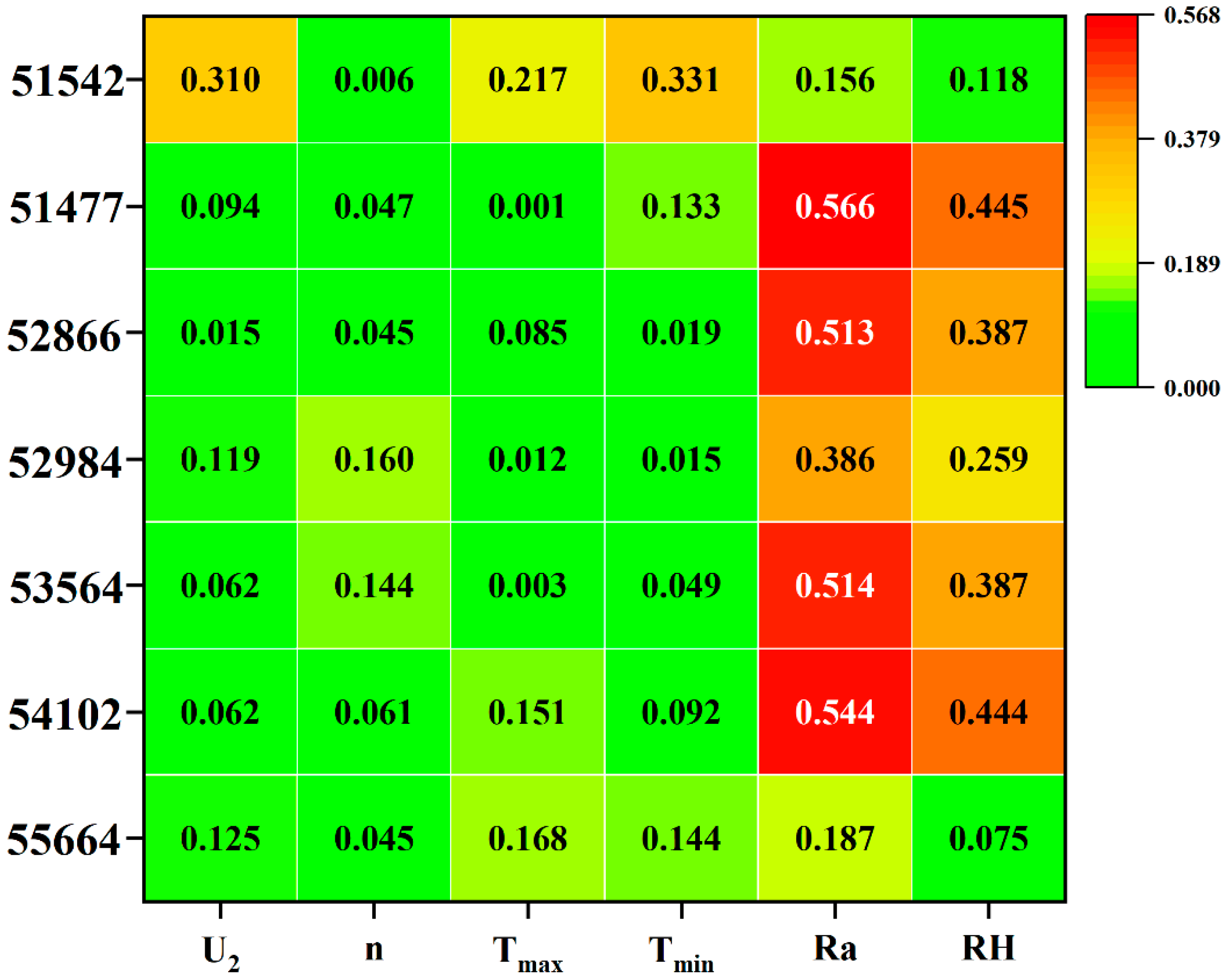
When limited by the equipment conditions of meteorological stations, many regions can obtain fewer types of meteorological data. The study used the sensitivity analysis method to make a preliminary qualitative analysis of ETO calculated by the PM formula. Figure 4 shows the sensitivity coefficient of various meteorological factors to PM. Ra, RH, and Tmax are the first three factors sensitive to PM. In most sites, Ra has the highest sensitivity to PM, which means that Ra significantly affects ETO. However, sensitivity analysis has some limitations in solving nonlinear and complex problems. Therefore, in this study, a partial correlation analysis algorithm is used to calculate the correlation between meteorological factors and ETO, and high correlation factors are selected as input factors for different stations. The correlation between meteorological factors of each station and ETO is shown in Figure 5. Ra is the primary factor affecting ETO prediction in almost all stations (except Dingri stations), and its Pearson correlation coefficient ranges from 0.187 to 0.566. Ra is an important calculation parameter of the FAO56 PM formula, and this analysis precisely demonstrates the significance of the energetic terms in the evapotranspiration process [37]. Many models can only estimate ETO by inputting data on radiation [23]. The influence of RH on the ETO model is second only to Rs, and its PCCs coefficient ranges from 0.259 to 0.480. The greater impact that RH had on the ETO results was also revealed in Fan et al. [38]. In this study, the Pearson correlation coefficient of temperature (Tmax, or Tmin) ranks in the top three for all stations (excluding Dingri only), and the range of PCCs coefficients is 0.085–0.331. Many studies also show that temperature (Tmax, or Tmin) has had a great impact on ETO in recent years, consistent with the conclusion of this study [39,40]. U2 and n have little influence on ETO estimation, and the sum of PCCs coefficients of the two factors is less than 0.147. The law of the main factors of the Dingri site is very different from that of other sites. U2 shows a significant impact that is inconsistent with other sites, and the influence of the Tmin factor on the ETO of this site is also much higher than that of other sites. The station is located in the Gangba basin and at the foot of the Himalayan Mountains. The local diurnal temperature difference is large (annual temperature difference is 22.1 °C; daily temperature difference is 18.2 °C), and the extreme lowest temperature is often lower than 27 °C, which may be the reason why the correlation coefficient of Tmin is greater than Ra. The PCCs coefficient of U2 is 0.3096 at the Dingri station, but the coefficient range at other stations is 0.015–0.095. The two meteorological factors (U2 and Tmin) at the Tingri station vary greatly during the year, resulting in Tmin and U2 becoming the key correlation factors to ETO, but the main related factors of most stations are Ra, RH, and temperature.
The impacts of meteorological factors obtained from partial correlation analysis of ETO estimation is sorted. The top three, four, and five factors in terms of contribution rate were used to construct the input combination.

3.2. Analysis of ELM Model Predicting Daily Evapotranspiration

An ELM model and hybrid model based on ELM and optimization algorithms (GEO-KELM and SSA-ELM) were established after determining the main meteorological factors. The top three, four, and five factors in the main factor analysis results are considered model inputs, and ETO was viewed as the output. The accuracy level of the ETO test values is significantly dependent on input factors and the type of model.
The combination of factors extracted by the Pearson coefficient is input into the three ETO models. The performance of the model is shown in Figure 6, and the statistical values of ETO models are shown in Table 2. The estimation accuracy of the independent ELM model was better in most sites, with RMSE = 0.197–1.395, R2 = 0.760–0.972, MAE = 0.147–1.139, and NSE = 0.756–0.972. The increase in input factors can improve the precision of the model, but not significantly. When the model input the top five factors of the PCCs coefficient, the accuracy index range of ELM model was RMSE = 0.174–1.245, R2 = 0.804–0.983, MAE = 0.135–0.985, and NSE = 0.804–0.983. The ELM model shows a better estimation ability and stability than the empirical model [41], mainly because ETO estimation is a complex nonlinear process. The empirical model has great limitations in solving nonlinear problems. Gocic et al. [42] applied 20 years of meteorological data on Serbia to build an ETO model based on ELM and a variety of empirical formulas, and the results showed that the estimation accuracy of ELM was better than that of the empirical model. However, the selection of kernel functions and parameter settings in the ELM model is not optimal, which causes some errors in the model results. Compared with the independent ELM, the optimized hybrid model with the same input factors obtained better advantages, which indicated that the bionic optimization algorithms (GEO and SSA) had good optimization effects on the ELM model. Among the two mixed models, the accuracy of the SSA-ELM model was higher, RMSE = 0.076–1.326, R2 = 0.785–0.999, MAE = 0.060–1.084, and NSE = 0.782–0.999 (three factors), RMSE = 0.081–1.214, R2 = 0.817–0.999, MAE = 0.062–0.958, and NSE = 0.817–0.999 (four factors), RMSE = 0.067–0.085, R2 = 0.998–0.999, MAE = 0.050–0.066, and NSE = 0.998–0.999 (five factors). The accuracy of the mixed model was improved during the process of adding input factors. Based on the input of three factors, the estimation accuracy of the GEO-ELM and SSA-ELM models was significantly improved when the fourth factor, ranked by PCCs, was added. The resulting being RMSE = 0.132–0.952, R2 = 0.813–0.996, MAE = 0.223–1.079, and NSE = 0.813–0.996(GEO-ELM), RMSE = 0.081–1.214, R2 = 0.817–0.999, MAE = 0.062–0.958, and NSE = 0.817–0.999(SSA-ELM).
All ETO models achieved the highest accuracy compared to other input combinations when the top five factors of PCCs coefficients were put into the model. In the case of gradually increasing input factors, the accuracy of the independent ELM model was improved to some extent: RMSE = 0.067–0.085, R2 = 0.998–0.999, MAE = 0.050–0.066, and NSE = 0.998–0.999. The ETO estimated by the two mixed models at the input of five factors had a strong goodness of fit with the ETO calculated by FAO56-PM, and SSA-ELM performed better: RMSE = 0.067–0.085, R2 = 0.998–0.999, MAE = 0.050–0.066, and NSE = 0.998–0.999. The results show that the two biological heuristic optimization algorithms can improve the estimation accuracy and stability of the ELM model. In the latest studies, some scholars combined GBDT algorithm and PSO algorithm to predict ETO (R2 = 0.63–0.84), but the accuracy was significantly lower than the hybrid model (SSA-ELM) in this study [43]. Zhu et al. used the PSO-ELM model to estimate the daily ETo in the arid region of Northwest China, and the accuracy of the model (R2 = 0.85–0.96) was lower than that of the SSA-ELM model proposed in this study [44]. Zhao et al. proposed the CS-Elman model to estimate ETO. In contrast, the hybrid model recommended in this study is more efficient than the CS-Elman model [39].
In this study, partial correlation analysis can efficiently select the factors with a large impact on the ETO model. All three models have a satisfactory estimation accuracy when the top three PCCs factors are taken as the main inputs of the model. When the fourth influencing factor is added as input, the mean values of the RMSE, R2, MAE and NSE of the three models are improved, respectively: 0.20%, 1.60%, 0.20%, 0.80%, (ELM), 46.55%, 3.88%, 47.54%, 4.06%(GEO-ELM), 46.55%, 3.88%, 47.50%,4.16%(SSA-ELM). When the fifth influencing factor is added as an input on the basis of the input of the four factors, the mean values of RMSE, R2, MAE and NSE of the three models are improved, respectively: 2.80%, 2.80%, 4.10%, 3.80%, (ELM), 5.07%, 0.03%, 5.00%, 0.38%, (GEO-ELM), 5.07%, 0.38%, 4.95%, 0.05%(SSA-ELM). The test results show that the accuracy of the three models is slightly improved when the input of the fourth factor is added. When the fifth influencing factor was added to the ETO model as input, the independent ELM model still showed a small improvement in accuracy. However, the performance of the hybrid model (GEO-ELM and SSA-ELM) is very different from that of the independent ELM model. The accuracy and stability of the hybrid model are greatly improved when the fifth influencing factor is added as the input, and the estimated ETO value is extremely close to the standard value calculated by FAO56.

3.3. Applicability of ETO Model in Semi-Arid Region

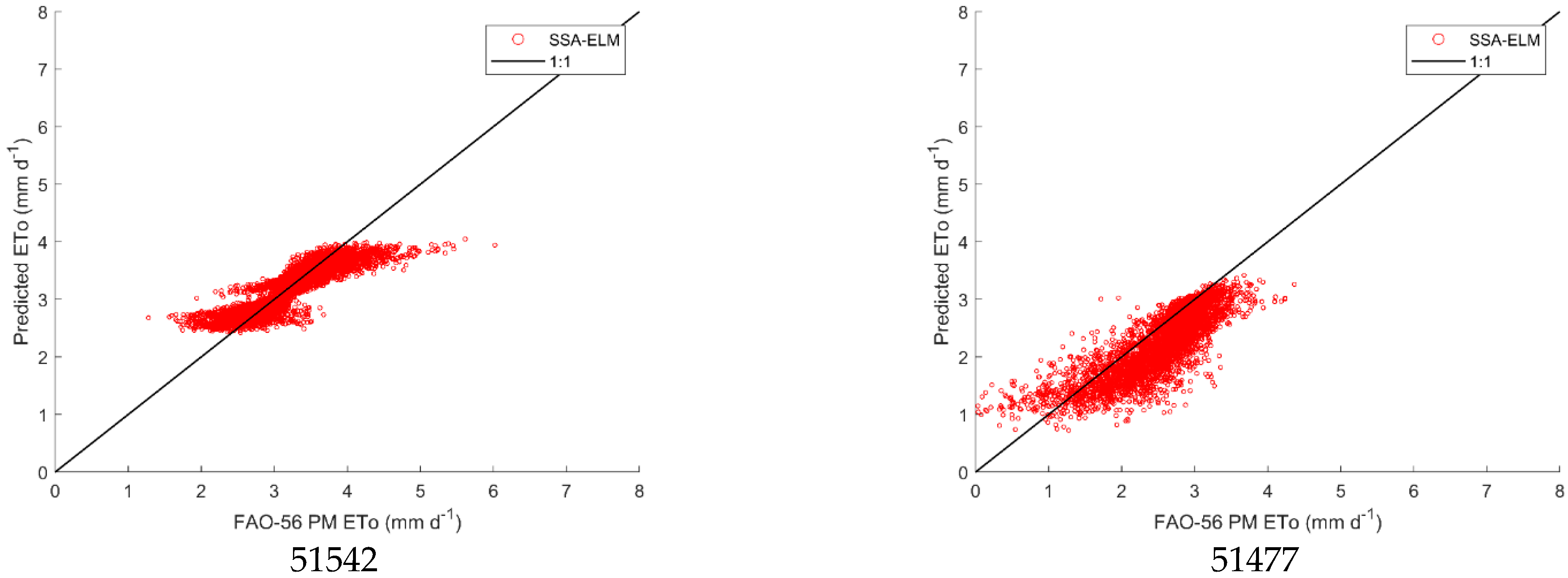
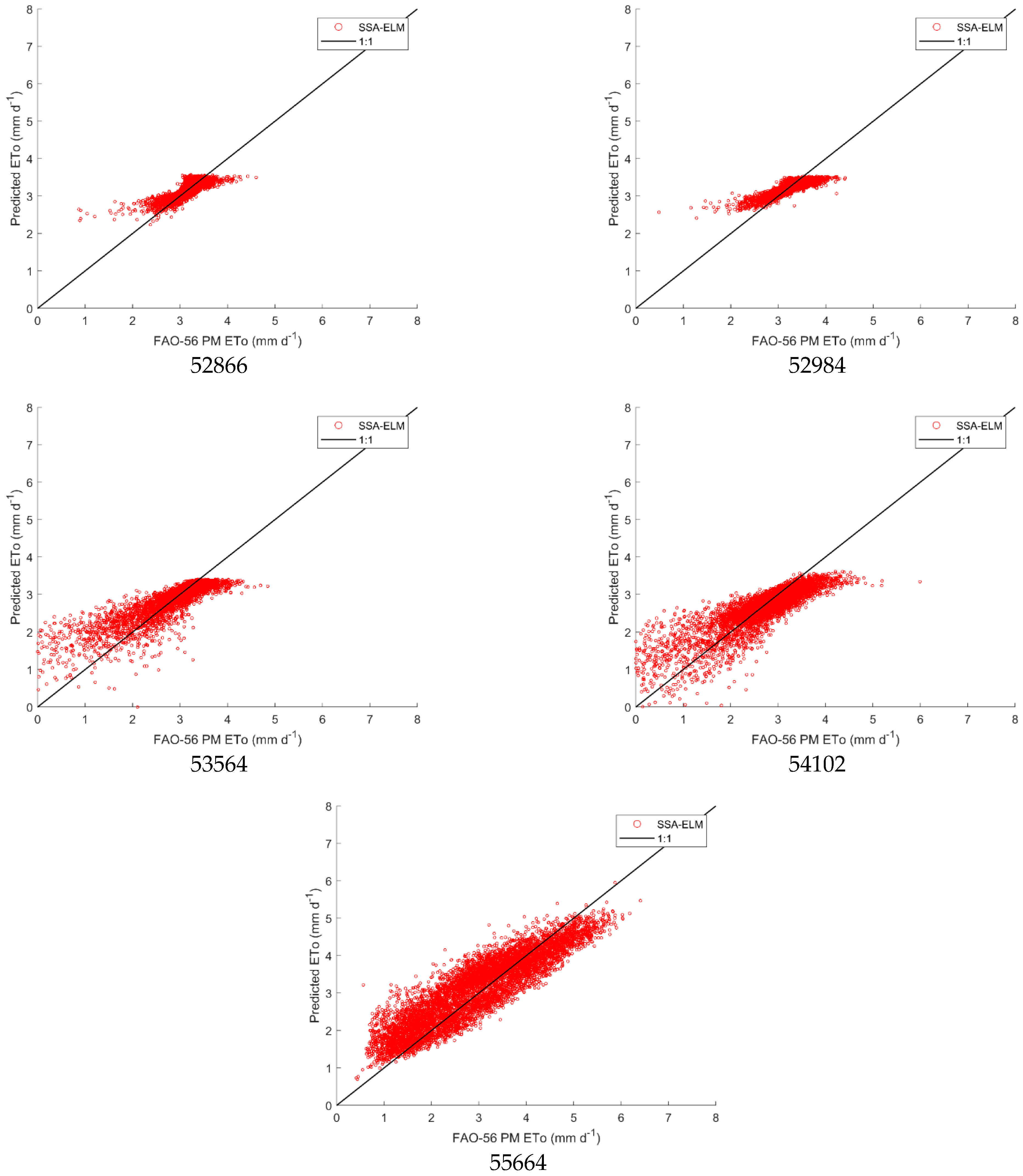
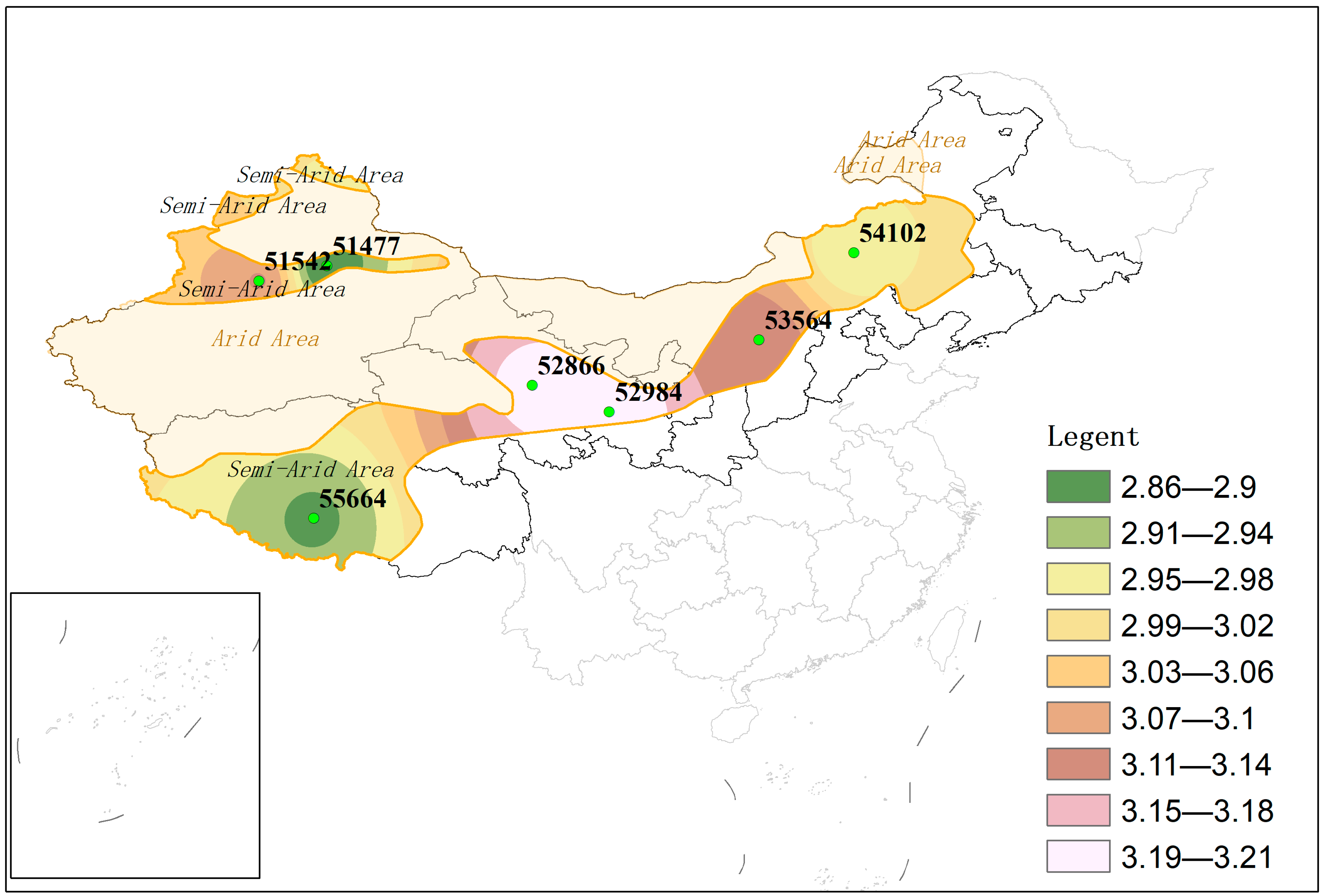
When different factor combinations were input into the model, the statistical performance of the Elm model and hybrid model (Geo-ELM and SSA-KELM) at seven stations in the semi-arid region was represented by a comprehensive evaluation index GPI (Table 3). The visual performance of the evaluation index is shown in Figure 4. The performance of the three ETO models at different sites is very similar when the main factors selected by the partial correlation analysis method are used to construct the estimation model. When the three factors were input to build the model, the ETO model performed better in Hequ, Xilinhot, and Dingri stations, and the GPI range of the three models was as follows: 1.514–1.589 (ELM), 1.722–1.800 (GEO-ELM), 1.750–1.980 (SSA-ELM). The three ETO models performed poorly in other sites, and the distribution range of the GPI index was −2.000–0.928. Compared with the independent ELM model, GEO-ELM and SSA-KELM models have better stability in different sites. When three factors were input, the GPI of all three ETO models improved at each site. When four factors were input, the performance of the ETO model at different sites was consistent with that when three factors were input. The performance of the ETO model at the Hequ, Xilinhot, and Dingri sites was better. The GPI range of the three models is as follows: 1.579–1.613 (ELM), 1.739–1.815 (GEO-ELM), 1.795–1.1.973 (SSA-ELM). When five factors were input to build the model, the independent ELM model only improved the accuracy at some sites, while the stability of the mixed model was significantly improved in different sites. Both hybrid models were able to very accurately estimate ETO at all seven sites. When the top five PCCs factors were input to the mixed model as the input combination, the GPI ranges were 1.739–1.936 (GEO-ELM) and 1.795–2.000 (SSA-ELM). Comparing the two hybrid models, the SSA-ELM model had the best adaptability at seven sites in semi-arid regions. Figure 7 shows a comparison between the estimation result of the SSA-ELM model and the standard value of FAO56-PM when five factors are input. The GEO algorithm easily falls into the local optimal value, and the convergence speed is slow. The accuracy of the GEO-ELM model is still slightly poor in some sites. In the process of SSA algorithm optimization, part of the population will randomly update the location, which makes the algorithm struggle to obtain the local optimal solution. This method to avoid falling into the local optimal solution is like the Levey flight in the cuckoo optimization algorithm [39], and the step size of Levi’s flight conforms to the heavy tail distribution. Therefore, a small number of individuals find the global optimal solution. The hybrid of the SSA optimization algorithm and the ELM model has high efficiency and stability, and there are many similar conclusions in previous studies. Zhou et al. [45] applied a combination of the SSA algorithm and ELM model to predict carbon price and compared this with a variety of machine learning models (BP, LSSVM, GA-ELM, etc.). The results show that the SSA-ELM model is much better than other models in terms of stability and prediction accuracy. The spatial map of ETO estimated by the recommended model in the most recent year (2019) is shown in Figure 8.

4. Conclusions

This study combined the PCA method and machine learning algorithms (ELM, GEO-ELM, and SSA-ELM) to construct ETO estimation models with limited factors in the semi-arid region of China. The results show that:
(1) When calculating the influence of meteorological factors on the ETO model based on partial correlation analysis, Ra is the primary factor affecting ETO model, and its importance range is 0.187–0.566. Additionally, RH and temperature are the main factors in ETO model construction;
(2) The optimization algorithms (GEO and SSA) have a good optimization effect on the ELM model’s estimation ability, and the SSA-ELM model has higher estimation accuracy than the GEO model. When five factors are input, the ETO estimated by SSA-ELM is very close to the standard value calculated by FAO56 PM, RMSE = 0.067–0.085, R2 = 0.998–0.999, MAE = 0.050–0.066, and NSE = 0.998–0.999;
(3) When using meteorological data from different stations to build models, the mixed model had better stability than the independent ELM model. The SSA-ELM model had the highest estimation accuracy and stability at seven sites in semi-arid regions of China.
In recent years, using the measurement method based on satellites to estimate regional evapotranspiration has been important research. In future research, we will combine satellite data to conduct a global scale ETO model applicability study on the hybrid model [7,46,47].

Author Contributions

Conceptualization: X.Z.; methodology: X.Z. and Z.Q.; software: Y.L. and J.B.; validation: Z.Z. and G.F.; data curation: Z.Z. and J.Z.; writing—original draft preparation: X.Z. and G.F.; writing—review and editing: Z.Z. and Y.W.; visualization: X.Z. and Z.Q.; supervision: Z.Q. and X.X. All authors have read and agreed to the published version of the manuscript.

Funding

This work was supported by National Natural Science Foundation of China (grant No. 51809217).

Institutional Review Board Statement

Not applicable.

Informed Consent Statement

Not applicable.

Data Availability Statement

The data used in this paper can be provided by Xinbo Zhao ([email protected]).

Conflicts of Interest

The authors declare that they have no known competing financial interests or personal relationships that could have appeared to influence the work reported in this paper.

References

  1. Zhang, Q.; Xu, C.; Chen, X. Reference evapotranspiration changes in China: Natural processes or human influences. Theor. Appl. Climatol. 2011, 103, 479–488. [Google Scholar] [CrossRef]
  2. Miralles, D.; De Jeu, R.; Gash, J.; Holmes, T.; Dolman, A. Magnitude and variability of land evaporation and its components at the global scale. Hydrol. Earth Syst. 2011, 15, 967–981. [Google Scholar] [CrossRef] [Green Version]
  3. Awad, M.; Darwish, T. Mapping evapotranspiration to administer water use in Bekaa valley. In Proceedings of the 2015 International Workshop on Evapotranspiration Mapping for Water Security, Washington, DC, USA, 15–17 September 2015. [Google Scholar]
  4. Allen, G.; Pereira, S.; Raes, D.; Smith, M. Crop Evapotranspiration-Guidelines for Computing Crop Water Requirements-FAO Irrigation and Drainage Paper 56. FAO Rome 1998, 300, D05109. [Google Scholar]
  5. Gavil´an, P.; Berengena, J.; Allen, G. Measuring versus estimating net radiation and soil heat flux: Impact on Penman-Monteith reference ET estimates in semiarid regions. Agric. Water Manag. 2007, 89, 275–286. [Google Scholar] [CrossRef]
  6. L´opez-Urrea, R.; Olalla, S.; Fabeiro, C.; Moratalla, A. An evaluation of two hourly reference evapotranspiration equations for semiarid conditions. Agric. Water Manag. 2006, 86, 277–282. [Google Scholar] [CrossRef]
  7. Srivastava, A.; Sahoo, B.; Raghuwanshi, S.; Singh, R. Evaluation of variable-infiltration capacity model and MODIS-terra satellite-derived grid-scale evapotranspiration estimates in a river basin with tropical monsoon-type climatology. J. Irrig. Drain. Eng. 2017, 143, 04017028.1–04017028.16. [Google Scholar] [CrossRef] [Green Version]
  8. Elbeltagi, A.; Kumari, N.; Dharpure, K.; Mokhtar, A.; Kuriqi, A. Prediction of combined terrestrial evapotranspiration index (ctei) over large river basin based on machine learning approaches. Water 2021, 13, 547. [Google Scholar] [CrossRef]
  9. Nasseri, S.; Ghamarnia, H.; Khosravi, R.; Mohamadi, Y.; Sargordi, F. Evaluation of the accuracy of different combined methods for estimating the potential evapotranspiration in different climates (case study: Iran). Water Irrig. Manag. 2020, 10, 443–452. [Google Scholar]
  10. Sinclair, T. “Natural Evaporation from Open Water, Bare Soil and Grass” by Harold L. Penman, (1948) A193:120–146. Crop Sci. 2019, 59, 2297–2299. [Google Scholar] [CrossRef]
  11. Biazar, S.; Dinpashoh, Y.; Singh, V. Sensitivity analysis of the reference crop evapotranspiration in a humid region. Environ. Sci. Pollut. Res. 2019, 26, 32517–32544. [Google Scholar] [CrossRef] [PubMed]
  12. Yu, F.; Yue, J.; Ningbo, C.; Lu, Z.; Chen, L.; Daozhi, G. Calibration of Hargreaves model for reference evapotranspiration estimation in Sichuan basin of southwest China. Agric. Water Manag. 2017, 181, 1–9. [Google Scholar]
  13. Hafeez, M.; Chatha, Z.; Khan, A.; Gulshan, A.; Basit, A.; Tahira, F. Comparative Analysis of Reference Evapotranspiration by Hargreaves and Blaney-Criddle Equations in Semi-Arid Climatic Conditions. Curr. Res. Agric. Sci. 2020, 7, 52–57. [Google Scholar] [CrossRef]
  14. Yang, Y.; Luo, Y.; Wu, C.; Zheng, H.; Zhang, L.; Cui, Y.; Sun, N.; Wang, L. Evaluation of six equations for daily reference evapotranspiration estimating using public weather forecast message for different climate regions across China. Agric. Water Manag. 2019, 222, 386–399. [Google Scholar] [CrossRef]
  15. Fernando, F.; Fernando, F.; Marco, A.; Epitácio, J. Performance of estimative models for daily reference evapotranspiration in the city of Cassilândia, Brazil. Eng. Agric. 2017, 37, 173–184. [Google Scholar]
  16. Irmak, S.; Irmak, A.; Allen, R.G.; Jones, J.W. Solar and net radiation-based equations to estimate reference evapotranspiration in humid climates. J. Irrig. Drain. Eng. 2003, 129, 336–347. [Google Scholar] [CrossRef]
  17. Shakibul, I.; Rashidul, A. Performance evaluation of FAO Penman-Monteith and best alternative models for estimating reference evapotranspiration in Bangladesh. Heliyon 2021, 7, e07487. [Google Scholar]
  18. Hossein, T.; Ozgur, K.; Azadeh, E.; Hosseinzadeh, T. SVM, ANFIS, regression and climate based models for reference evapotranspiration modeling using limited climatic data in a semi-arid highland environment. J. Hydrol. 2012, 444–445, 78–89. [Google Scholar]
  19. Akpootu, D.; Iliyasu, M. A comparison of various evapotranspiration models for estimating reference evapotranspiration in Sokoto, North Western, Nigeria. Phys. Sci. Int. J. 2017, 14, 1–14. [Google Scholar] [CrossRef]
  20. Valiantzas, J. Temperature-and humidity-based simplified Penman’s ETO formulae. Comparisons with temperature-based Hargreaves-Samani and other methodologies. Agric. Water Manag. 2018, 208, 326–334. [Google Scholar] [CrossRef]
  21. Shrestha, N.; Shukla, S. Support vector machine based modeling of evapotranspiration using hydro-climatic variables in a sub-tropical environment. Agric. For. Meteorol. 2015, 200, 172–184. [Google Scholar] [CrossRef]
  22. Junliang, F.; Wenjun, Y.; Lifeng, W.; Fucang, Z.; Huanjie, C.; Xiukang, W.; Xianghui, L.; Youzhen, X. Evaluation of SVM, ELM and four tree-based ensemble models for predicting daily reference evapotranspiration using limited meteorological data in different climates of China. Agric. For. Meteorol. 2018, 263, 225–241. [Google Scholar]
  23. Wu, Z.; Cui, N.; Zhu, B.; Zhao, L.; Wang, X.; Hu, X.; Wang, Y.; Zhu, S. Improved hargreaves model based on multiple intelligent optimization algorithms to estimate reference crop evapotranspiration in humid areas of southwest China. Atmosphere 2020, 12, 15. [Google Scholar] [CrossRef]
  24. Mohammadi, B.; Mehdizadeh, S. Modeling daily reference evapotranspiration via a novel approach based on support vector regression coupled with whale optimization algorithm. Agric. Water Manag. 2020, 237, 106145. [Google Scholar] [CrossRef]
  25. Lu, X.; Fan, J.; Wu, L.; Dong, J. Forecasting multi-step ahead monthly reference evapotranspiration using hybrid extreme gradient boosting with grey wolf optimization algorithm. Comput. Model. Eng. Sci. 2020, 125, 699–723. [Google Scholar] [CrossRef]
  26. Citakoglu, H.; Cobaner, M.; Haktanir, T.; Kisi, O. Estimation of Monthly Mean Reference Evapotranspiration in Turkey. Water Resour. Manag. 2014, 28, 99–113. [Google Scholar] [CrossRef]
  27. Chia, M.; Huang, Y.; Koo, C. Reference evapotranspiration estimation using adaptive neuro-fuzzy inference system with limited meteorological data. In IOP Conference Series: Earth and Environmental Science; IOP Publishing: Tokyo, Japan, 2020; Volume 612, p. 012017. [Google Scholar]
  28. Han, Y.; Wu, J.; Zhai, B.; Pan, Y.; Zeng, W. Coupling a bat algorithm with xgboost to estimate reference evapotranspiration in the arid and semiarid regions of China. Adv. Meteorol. 2019, 2019, 9575782. [Google Scholar] [CrossRef]
  29. Zhang, Y.; Wei, Z.; Zhang, L.; Lin, Q.; Du, J. Improved online sequential extreme learning machine for simulation of daily reference evapotranspiration. Tecnol. Cienc. Agua 2017, 8, 127–140. [Google Scholar] [CrossRef]
  30. Samui, P.; Dixon, B. Application of support vector machine and relevance vector machine to determine evaporative losses in reservoirs. Hydrol. Processes 2012, 26, 1361–1369. [Google Scholar] [CrossRef]
  31. Ahmad, M.J.; Choi, K.S. Influence of climate variables on FAO Penman-Monteith reference evapotranspiration in the Upper Chenab Canal command area of Pakistan. Paddy Water Environ. 2018, 16, 425–438. [Google Scholar] [CrossRef]
  32. Cui, F.; Zhang, H.; Yao, Q. Influencing factors and prediction models of soil temperature in Yantai based on partial correlation analysis. Shandong Agric. Sci. 2010, 1, 18–21. [Google Scholar]
  33. Abdullah, S.; Malek, A.; Abdullah, S.; Kisi, O.; Yap, S. Extreme learning machines: A new approach for prediction of reference evapotranspiration. J. Hydrol. 2015, 527, 184–195. [Google Scholar] [CrossRef]
  34. Mohammadi-Balani, A.; Nayeri, M.; Azar, A.; Taghizadeh-Yazdi, M. Golden eagle optimizer: A nature-inspired metaheuristic algorithm. Comput. Ind. Eng. 2021, 152, 107050. [Google Scholar] [CrossRef]
  35. Yan, P.; Shang, S.; Zhang, C.; Yin, N. Research on the Processing of Coal Mine Water Source Data by Optimizing BP Neural Network Algorithm with Sparrow Search Algorithm. IEEE Access 2021, 9, 108718–108730. [Google Scholar] [CrossRef]
  36. Feng, Y.; Peng, Y.; Cui, N.; Gong, D.; Zhang, K. Modeling reference evapotranspiration using extreme learning machine and generalized regression neural network only with temperature data. Comput. Electron. Agric. 2017, 136, 71–78. [Google Scholar] [CrossRef]
  37. Yu, H.; Wen, X.; Li, B.; Yang, Z.; Wu, M.; Ma, Y. Uncertainty analysis of artificial intelligence modeling daily reference evapotranspiration in the northwest end of China. Comput. Electron. Agric. 2020, 176, 105653. [Google Scholar] [CrossRef]
  38. Fan, J.; Wu, L.; Zhang, F.; Xiang, Y.; Zheng, J. Climate change effects on reference crop evapotranspiration across different climatic zones of China during 1956. J. Hydrol. 2016, 542, 923–937. [Google Scholar] [CrossRef]
  39. Zhao, L.; Zhao, X.; Pan, X.; Shi, Y.; Qiu, Z.; Li, X.; Xing, X.; Bai, J. Prediction of daily reference crop evapotranspiration in different Chinese climate zones: Combined application of key meteorological factors and Elman algorithm. J. Hydrol. 2022, 610, 127822. [Google Scholar] [CrossRef]
  40. Xing, X.; Liu, Y.; Zhao, W.; Kang, D.; Yu, M.; Ma, X. Determination of dominant weather parameters on reference evapotranspiration by path analysis theory. Comput. Electron. Agric. 2016, 120, 10–16. [Google Scholar] [CrossRef]
  41. Feng, Y.; Cui, N.; Zhao, L.; Hu, X.; Gong, D. Comparison of ELM, GANN, WNN and empirical models for estimating reference evapotranspiration in humid region of Southwest China. J. Hydrol. 2016, 536, 376–383. [Google Scholar] [CrossRef]
  42. Gocic, M.; Petković, D.; Shamshirband, S.; Kamsin, A. Comparative analysis of reference evapotranspiration equations modelling by extreme learning machine. Comput. Electron. Agric. 2016, 127, 56–63. [Google Scholar] [CrossRef]
  43. Zhao, L.; Zhao, X.; Zhou, H.; Wang, X.; Xing, X. Prediction model for daily reference crop evapotranspiration based on hybrid algorithm and principal components analysis in Southwest China. Comput. Electron. Agric. 2021, 190, 106424. [Google Scholar] [CrossRef]
  44. Zhu, B.; Feng, Y.; Gong, D.; Jiang, S.; Zhao, L.; Cui, N. Hybrid particle swarm optimization with extreme learning machine for daily reference evapotranspiration prediction from limited climatic data. Comput. Electron. Agric. 2020, 173, 105430. [Google Scholar] [CrossRef]
  45. Zhou, J.; Chen, D. Carbon price forecasting based on improved CEEMDAN and extreme learning machine optimized by sparrow search algorithm. Sustainability 2021, 13, 4896. [Google Scholar] [CrossRef]
  46. Srivastava, A.; Rodriguez, J.; Saco, P.; Kumari, N.; Yetemen, O. Global Analysis of Atmospheric Transmissivity Using Cloud Cover, Aridity and Flux Network Datasets. Remote Sens. 2021, 13, 1716. [Google Scholar] [CrossRef]
  47. Kumar, U.; Srivastava, A.; Kumari, N.; Sahoo, B.; Chatterjee, C.; Raghuwanshi, N. Evaluation of spatiotemporal evapotranspiration using satellite-based approach and lysimeter in the agriculture dominated catchment. J. Indian Soc. Remote Sens. 2021, 49, 1939–1950. [Google Scholar] [CrossRef]
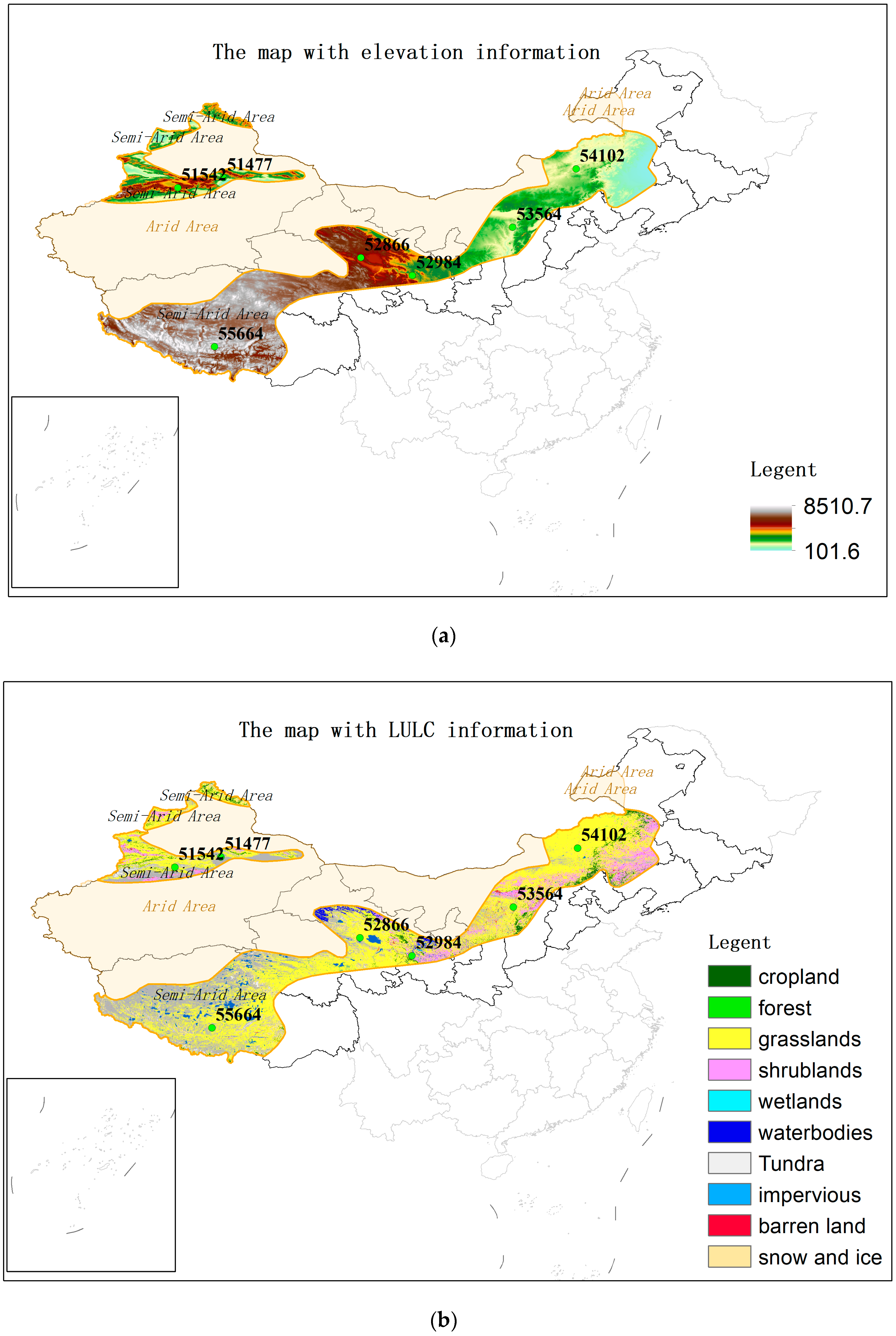
Figure 1. Site distribution map of the study area.
Atmosphere 13 00922 g001
Figure 2. Raw data preprocessing.
Atmosphere 13 00922 g002
Figure 3. Process of heuristic algorithms to optimize ELM models.
Atmosphere 13 00922 g003
Figure 4. Sensitivity analysis of different factors to ETO.
Atmosphere 13 00922 g004
Figure 5. PCCs coefficient of meteorological factors to ETO.
Atmosphere 13 00922 g005
Figure 6. Performance of the three ETO models.
Atmosphere 13 00922 g006aAtmosphere 13 00922 g006b
Figure 7. Scatter plots of predicted ETO values using SSA-ELM model against their corresponding FAO56-PM values when entering five factors.
Atmosphere 13 00922 g007aAtmosphere 13 00922 g007b
Figure 8. The spatial map of ETO estimated by the recommended model in 2019.
Atmosphere 13 00922 g008
Table 1. Geographical locations and mean daily values of the meteorological data.
Station IDStation NameLatitude
(°N)
Longitude
(°E)
Tmax
(°C)
Tmin
(°C)
RH
(%)
U2
(m s−1)
n
(h d−1)
ETO
(mm d−1)
51542Bayinbuluke42.584.73.3−10.50.72.77.61.7
51477Dabancheng43.388.313.1−1.10.32.68.43.1
52866Xining36.6101.714.10.10.51.57.22.4
52984Linxia35.6103.214.51.70.61.36.52.3
53564Hequ39.4111.116.12.00.51.57.32.5
54102Xilinhaote44.1116.110.0−3.60.53.48.02.6
55664Dingri28.687.111.7−5.20.42.59.12.86
Table 2. Statistical values of the three ETO models with different input parameters.
Three-Factor Input
StationELMGEO-ELMSSA-ELM
RMSER2MAENSERMSER2MAENSERMSER2MAENSE
515420.2950.6910.2060.6720.1070.9750.0870.9750.1040.9990.0780.999
514770.4180.6300.2670.4060.1530.9730.1280.9590.1480.9960.1160.996
528660.1690.5350.1130.4560.1950.9710.1640.9570.1890.9940.1490.994
529840.1800.5780.1170.5160.1800.9720.1460.9580.1740.9950.1330.995
535640.4290.6810.2330.6320.1960.9710.1650.9710.1900.9950.1500.995
541020.6780.6120.3840.5550.1910.9730.1540.9320.1850.9960.1400.996
556640.2300.6640.1520.5151.1420.7180.9740.6711.1060.7360.8820.717
Four-Factor Input
StationELMGEO-ELMSSA-ELM
RMSER2MAENSERMSER2MAENSERMSER2MAENSE
515420.2950.6890.2070.6700.1070.9750.0860.9750.1030.9990.0780.999
514770.4180.6300.2660.4080.1530.9730.1270.9590.1480.9960.1150.996
528660.1710.5350.1130.4460.1700.9720.1420.9580.1640.9960.1290.996
529840.1810.5720.1170.5110.1800.9720.1460.9580.1740.9950.1320.995
535640.4280.6770.2320.6330.1900.9720.1580.9720.1840.9950.1440.995
541020.6780.6090.3850.5540.1910.9730.1540.9320.1850.9960.1390.996
556640.2330.6080.1540.4980.1680.9710.1410.9300.1630.9940.1280.994
Five-Factor Input
StationELMGEO-ELMSSA-ELM
RMSER2MAENSERMSER2MAENSERMSER2MAENSE
515420.2660.7410.1870.7250.1070.9750.0860.9720.1030.9950.0780.999
514770.4160.6420.2560.4120.1470.9730.1230.9550.1430.9920.1120.996
528660.1660.5410.1090.4750.1510.9730.1280.9560.1460.9930.1160.997
529840.1740.5980.1130.5400.1670.9730.1350.9540.1620.9920.1220.996
535640.4240.6780.2310.6380.1880.9720.1570.9690.1820.9910.1430.995
541020.6570.6320.3630.5740.1720.9730.1380.9270.1670.9930.1250.997
556640.2330.6060.1540.4980.1670.9710.1400.9250.1620.9900.1270.994
Table 3. GPI value and ranking of the three ETO models.
StationELM GEO-ELM SSA-ELM
GPIRankingGPIRankingGPIRanking
Three-factor input
51542−2.00063−1.74962−1.68761
51477−1.53360−1.33857−1.14752
52866−1.30356−1.08151−0.96345
52984−1.29455−1.07349−0.92842
535641.514351.722261.9802
541021.589321.800171.79219
556641.547341.754221.75023
Four-factor input
51542−1.46259−1.24754−1.20753
51477−1.07350−0.90140−0.74737
52866−1.04148−0.83939−0.76838
52984−1.03847−0.92441−0.65736
535641.579331.786201.9737
541021.613301.815161.81515
556641.593311.739251.79518
Five-factor input
51542−1.366581.936102.0001
51477−0.981461.859111.9765
52866−0.948441.849121.9793
52984−0.946431.831131.9764
535641.666291.784211.9669
541021.699271.816141.9738
556641.679281.747241.9736
Publisher’s Note: MDPI stays neutral with regard to jurisdictional claims in published maps and institutional affiliations.